


利用德国LaVision公司的层析粒子成像测速(Tomo-PIV)和时间分辨粒子成像测速(TR-PIV)系统,测量汽车活塞发动机内部瞬态湍流场并和理论分析预测结果进行比对。
方案详情

THE UNIVERSITY ofEDINBURGH Edinburgh Research Explorer On the turbulent flow in piston engines: coupling of statisticaltheory quantities and instantaneous turbulence Citation for published version: Zentgraf, F, Baum, E, Bohm, B, Dreizler, A & Peterson, B 2016, 'On the turbulent flow in piston engines:coupling of statistical theory quantities and instantaneous turbulence' Physics of Fluids, vol 28, no. 4,045108. DOI: 10.1063/1.4945785 Digital Object Identifier (DOI):10.1063/1.4945785 Link: Link to publication record in Edinburgh Research Explorer Document Version: Peer reviewed version Published In: Physics of Fluids General rights Copyright for the publications made accessible via the Edinburgh Research Explorer is retained by the author(s)and / or other copyright owners and it is a condition of accessing these publications that users recognise andabide by the legal requirements associated with these rights. Take down policy The University of Edinburgh has made every reasonable effort to ensure that Edinburgh Research Explorercontent complies with Uk legislation. If you believe that the public display of this file breaches copyright pleasecontact openaccess@ed.ac.uk providing details, and we will remove access to the work immediately andinvestigate your claim. On the turbulent flow in piston engines: coupling of statistical theory quantities andinstantaneous turbulence Florian Zentgraf,1 Elias Baum, Benjamin Bohm,2 Andreas Dreizler, and BrianPeterson3, a) )Fachgebiet Reaktiue Stromungen und Messtechnik (RSM), Center of Smart Interfaces (CSI), Technische Universitat Darmstadt,Jovanka-Bontschits-Strasse 2, 64287 Darmstadt, Germany 2)Fachgebiet Energie und Kraftwerkstechnik (EKT), Technische Universitat Darmstadt, Jovanka-Bontschits-Strasse 2, 64287 Darmstadt,Germany 3)Institute for Energy Systems, Department of Mechanical Engineering,School of Engineering, University of Edinburgh, The King’s Buildings,Mayfield Road, Edinburgh EH9 3JL, Scotland UK (Dated: 13 April 2016) Planar particle image velocimetry (PIV) and tomographic PIV (TPIV) measure-ments are utilized to analyze turbulent statistical theory quantities and the instan-taneous turbulence within a single-cylinder optical engine. Measurements are per-formed during the intake and mid-compression stroke at 800 and 1500 RPM. TPIVfacilitates the evaluation of spatially-resolved Reynolds stress tensor (RST) distri-butions, anisotropic Reynolds stress invariants, and instantaneous turbulent vorticalstructures. The RST analysis describes distributions of individual velocity fluctuationcomponents that arise from unsteady turbulent flow behavior as well as cycle-to-cyclevariability (CCV). A conditional analysis, for which instantaneous PIV images aresampled by their tumble center location, reveals that CCV and turbulence have sim-ilar contributions to RST distributions at the mean tumble center, but turbulenceis dominant in regions peripheral to the tumble center. Analysis of the anisotropicReynolds stress invariants reveals the spatial distribution of axisymmetric expansion,axisymmetric contraction, and 3D isotropy within the cylinder. Findings indicatethat the mid-compression flow exhibits a higher tendency toward 3D isotropy thanthe intake flow. A novel post-processing algorithm is utilized to classify the geometryof instantaneous turbulent vortical structures and evaluate their frequency of occur-rence within the cylinder. Findings are coupled with statistical theory quantities toprovide a comprehensive understanding of the distribution of turbulent velocity com-ponents, the distribution of anisotropic states of turbulence, and compare the turbu-lent vortical flow distribution that is theoretically expected to what is experimentallyobserved. The analyses reveal requisites of important turbulent flow quantities anddiscern their sensitivity to the local flow topography and engine operation. ( a)Electronic mail: brian.peterson@ed.ac.uk ) I. INTRODUCTION The physics of the turbulent in-cylinder flow in internal combustion (IC) piston engineshave captivated scientists and engine designers for several decades. Engine flows are oftenamongst the most-complicated flows in technical applications today; they are non-stationary,yet periodic, turbulent flows that undergo rapid compression, expansion and gas exchange,which includes combustion and, in the case of direct-injection (DI), two-phase flows withphase changel5. Engine flows are highly more relevant than the filling and emptying of thecylinder contents; they are responsible for describing the key processes of turbulence mixingand combustion that define the engine performance and efficiency. For spark-ignition (SI) engines, emphasis is placed on generating a large-scale, rotatingflow motion (known as tumble or swirl) containing kinetic energy. The large-scale tumblingflow, which has an axis of rotation perpendicular to the cylinder axis, is intrinsically instablenear the end of compression and leads to the tumble breakdown where the kinetic energyfrom the tumble motion is transferred to small-scale turbulence4,7. The resulting mean flowand turbulence uniquely describes thermal transport5,8,9, fuel-air preparation10-15, ignitionbehavior16,17, and flame- and species-transport18-20, which accurately describes the instan-taneous burning rate. The creation of an organized large-scale tumble rotation is challengedby varying initial conditions, periodically varying boundary conditions during the cycle, andstochastic flow events that result in large-scale cycle-to-cycle flow variations21. Particularlyin direct-injection engines, cycle-to-cycle flow variations (termed CCV) can lead to dras-tic changes in fuel-air distributions and flame transport, which if severe can lead to poorburning cycles that limit power output and increase fuel consumption11,13,14,22,23. Engine development with improvement of fuel economy and reduced emissions requirestools to accurately measure and predict the turbulent in-cylinder flow. Reynolds-averagedNavier-Stokes (RANS) and large-eddy simulations (LES) are powerful computational toolsto predict engine flows and are widely used for the design and optimization of enginedevelopment24-27. While RANS and LES simulations have provided valuable contributionstowards understanding engine flows, the difficulties in predicting flow physics for multipleoperating conditions and engine geometries is equally acknowledged. Model validation isneeded for any numerical tool modeling turbulent flows and the need for well-documentedvelocimetry measurements (e.g. Abraham et al.21, Baum et al.28, and Lacour and Pera29) is important for the development of more predictive engine models. Measurements that pro-vide distribution requisites of turbulent statistical theory quantities (e.g. Reynolds stresses)and can discern their sensitivities with regards to changes in engine operation (e.g. crank-angle, engine speed, inflow conditions) are well-sought after to provide useful metrics forcomparison between experiments and numerical simulations. Experiments utilizing laser Doppler anemometry (LDA) and particle image velocimetry(PIV) have been used extensively to understand the engine flow physics, with particularemphasis on turbulent flow generation and CCV30-34. Advances in diagnostics has led tothe ability to capture transient, multi-dimensional flow information within IC engines20,35-41.Just as planar PIV images of the instantaneous, spatially resolved velocity field was a warmwelcome from single-point, time-series LDA measurements, techniques like tomographic PIV(TPIV) are well-received to understand the three-dimensional (3D) flow behavior. As engineflows are inherently 3D, the ability to resolve the complete velocity gradient tensor becomesincreasingly important to analyze turbulent statistical theory quantities and instantaneousturbulent flow phenomena. Such capabilities are anticipated to provide further insight intothe study of turbulence and CCV as well as build more predictive models describing theengine flow that may deviate from traditional, fully-developed, isotropic, homogeneous tur-bulence assumptions commonly used for simulation platforms. In this study, planar PIV (denoted as PIV) and TPIV are applied to analyze turbulentstatistical theory quantities and the intantaneous turbulent flow within a single-cylinderoptical SI engine. This data extends from a comprehensive experimental database28 designedfor LES and RANS model development and validation purposes. The analysis focuses on theintake flow at 270° before top-dead center (bTDC) and mid-compression flow at 90°bTDCfor engine speeds of 800 and 1500 RPM. TPIV enables the evaluation of spatially-resolveddistributions of Reynolds stress tensors (RST), anisotropic Reynolds stress invariants, andinstantaneous turbulent vortical structures. Results from TPIV and PIV are compared toestablish data coherence. PIV measurements are also used to evaluate y-RST distributionsin a larger field-of-view (FOV). The RST analysis describes the distribution of individualvelocity fluctuation components arising from unsteady turbulent flow behavior and CCV (i.e.cyclic variances of the location and direction of mean flow features). A conditional analysisis introduced in attempt to calculate velocity fluctuations associated with turbulence andless biased by CCV. The local distribution of anisotropic Reynolds stress invariants reveals the spatial distribution of anisotropic states of turbulence existing within the cylinder. Toprovide analysis of the instantaneous turbulent flow, a box-counting algorithm (BCA) is usedto classify the shape of 3D vortical structures within the cylinder. This analysis providesa statistical view on instantaneous turbulence that is not based from statistical moments.but rather based on visualizations of the physical instantaneous vortical structures resolvedin the TPIV measurements.. Findings from the BCA are coupled with statistical theoryquantities to provide a comprehensive understanding of the turbulent velocity distribution,the anisotropic states of turbulence distribution, and compare the turbulent vortical flowdistribution that is theoretically expected to that which is experimentally observed. II. EXPERIMENTAL METHODOLOGY Planar PIV and TPIV measurements were performed in a single-cylinder DISI opticalengine operating under motored conditions (i.e. non-fired operation, see Table I).Theoptical engine and PIV diagnostics have previously been described in Baum et al.28 and aresummarized below. The optical engine features a twin-cam,overhead-valve pentroof cylinder head, a 55 mmheight quartz-glass cylinder liner with 8 mm window extension into the pentroof, and aBowditch piston arrangement with flat quartz-glass piston crown window (75 mm diameter).The cylinder head is equipped with a side-mounted fuel injector, centrally mounted sparkplug, and dual intake valves (33 mm diameter) and exhaust valves (29 mm diameter) locatedon opposite sides of the spark plug placement. The spark plug was removed and replacedwith a threaded plug and the injector remained inactive for the experiments. A stainlesssteel piping (1.4m length) extending from a sound reduction plenum is connected to thedual-port intake system via a Y-tube, which was specifically made by laser sintering toprovide simplified boundary surface geometries. The intake system was specially designed toprovide reproducible thermodynamic and flow boundary conditions and simplified meshingfor three-dimensional flow simulations. Further details of the intake port geometries as wellas detailed flow measurementss((water analog) for the inlet engine geometry are found inFreudenhammer et al.43,44 Velocimetry measurements were performed at two engine speeds (800 and 1500RPM)with 0.95 bar intake pressure and 23°C intake air temperature. Both intake ports remained Engine speed 800, 1500RPMIntake pressure 0.95 barIntake air temp. 23°CMass of air in 11.5,22.2kg/hrAir relative humidity 1.8%Flow motion TumbleCyl. head, coolant temp. 60°CEngine bore, stroke 86, 86 mmCompression ratio 8.5Disp. volume 499 mmIntake valve open 325°after TDCIntake valve close 125°bTDCExhaust valve open 105°after TDCExhaust valve close 345°bTDC TABLE I. Engine operating parameters. TDC refers to top-dead-center compression. active to produce a directed tumble flow motion within the engine.The intake air wasaccurately defined by mass flow controllers (Bronkhorst) supplied by a pressurized air sys-tem with relative humidity of 1.8%. The cycle averaged air flow rate into the engine was11.5kg/hr (800RPM) and 22.2kg/hr (1500RPM), which was measured with two identicalrotary piston gas flow meters (FM, Aerzen) within the intake and exhaust systems. Siliconeoil droplets (approx. 1 um diameter) were used as the seeding medium for the velocimetrymeasurements. The droplets were introduced into the intake air (1.4 m upstream the engine)via an aerosol generator (AGF-10.0,Palas). Adual-cavity frequency-doubled Nd:YAG laser (Edgewave INNICNNOSLABIS4 II-DE.532 nm, 8.0mJ/pulse) and 12-bit digital camera (Phantom V.711) were synchronized tothe engine at up to 13.3 Hz for PIV measurements.The camera imaged perpendicularlyonto a 65 ×60 mm²FOV within the central symmetry plane (i.e. z =0mm) (Fig. 1a,PIV camera shown in red). The PIV laser light sheet thickness was 1 mm. A dual-cavityfrequency-doubled Nd:YAG (PIV-400, Spectra Physics, 532 nm, 375 mJ/pulse) operating at3.3 Hz was used for TPIV measurements. Four 12-bit CCD cameras (ImagerIntense, LaV- ision) in Scheimpflug arrangement were setup circularly around the engine (Fig. 1a, Cams1-4) and each camera projection provided independent line-of-sight information of the illu-minated volume. TPIV measurements resolved the volumetric flow within a 47×35×8mmvolume centered in the tumble plane. The central plane of the TPIV volume (i.e. z=0mm)corresponds to the planar PIV measurement location. Laser pulse time separation (dt) wasspecified at the image timing to ensure that the maximum pixel shift was within 1/4 of thefinal PIV interrogation window size. Planar PIV and TPIV measurements were conducted in separate experiments at selectedcrank-angle degrees (CAD) during intake (270°bTDC) and compression (90°bTDC) fordifferent engine speeds (800 and 1500RPM). Planar PIV measurements were recorded upto 2700 consecutive cycles,while TPIV measurements were recorded for 300 cycles. Unlessotherwise stated, the planar PIV measurements in this work are presented for a 300 cyclesubset of the 2700 sequence to provide the same statistical sample size for PIV and TPIV. A. Velocity field processing A commercial software program (DaVis, LaVision) was used for PIV and TPIV process-ing. Images of a spatially defined target within the engine were used to calibrate imagesand match viewing planes from multiple cameras. For planar PIV, Mie scattering imageswere cross-correlated with decreasing-window, multi-pass iterations with 75 % window over-lap. This provided a 2.0 mm spatial resolution based on the final interrogation window size(32 × 32 pixels) with a vector spacing of 0.63mm.This considers a spatial resolution of80% of the final interrogation window size when 75 % overlap is utilized. A 3×3 Gaussiansmoothing filter operation was applied to the vector field to remove noise at the spatialscales near the resolution limit of the PIV. For TPIV, a volume self-calibration45 was performed for each CAD imaged and provideda remaining pixel disparity of less than 0.3 pixels for all cameras. The reconstruction of the3D particle images was performed using an iterative multiplicative algebraic reconstructiontechnique (MART) algorithm46 yielding approximately 200 volumes in the z-direction withan average particle density of 0.042 particles per pixel. A volume cross-correlation withdecreasing volume size (final size: 64 × 64 ×64pixels) with 75 % overlap was applied andprovided a spatial resolution of 1.76 mm with vector spacing of 0.55 mm in all directions. This considers a spatial resolution of 80% of the final interrogation window size when 75%overlap is utilized. A 3 ×3×3 Gaussian smoothing filter was applied to the vector field toremove noise below the spatial resolution. Additional information regarding velocity fieldprocessing are discussed in Baum et al.28. B. Uncertainty of PIV measurements The identification of measurement uncertainty with digital PIV has been addressed withinprevious works45,47-53.AAcquiring reliable PIV data with minimal uncertainty is largelydepending on parameters such as:tracer particle, optical medium, camera settings, andchoice of PIV algorithm. Baum et al.28 discusses these in detail for the presented dataset.Overall, an accumulated uncertainty of approx. 5% has been stated for the presented PIVmeasurements28, while TPIV measurements presented have uncertainties up to 9%40,54. Uncertainty of velocity fluctuations calculated by Reynolds decomposition is pending onthe uncertainty of the velocity component itself and the standard error of the ensemble-mean.Baum et al.28 discusses the standard error of the ensemble-mean in detail. It is shown thatthis quantity is locally dependent for velocity datasets of finite sample sizes. Overall, it hasbeen shown that for 300 samples the local dependence is small and an uncertainty of themean in the order of 0.3 m/s for 270°bTDC and 0.2 m/s for 90°bTDC can be assumed. Thisis leading to an approximate 0.5% additional error on the velocity fluctuations due a samplesize of 300 cycles. III. ENSEMBLE-AVERAGE FLOW FIELDS Before discussing the analysis of statistical turbulent flow quantities, it is first importantto discuss the features of the in-cylinder flow at the CADs of interest. Figures 1b-e show theensemble-average flow field (z=0 mm) at 270°bTDC and 90°bTDC for 800RPM (b,c) and1500RPM (d,e). The flow field is composed from PIV images for 300 cycles. Streamlinesare used to show the flow direction, while the color-scale shows the velocity magnitude. Atthe CADs shown, the piston surface is located at y=-52mm. During intake, at 270°bTDC, the flow is characterized by high velocities entering thecylinder and the general formation of the clockwise tumble motion.1V1elocity magnitudes FIG. 1. (a) Experimental setup. Velocity magnitudes and streamlines of the ensemble-averagedflow within z=0 mm plane for (b) 270°bTDC 800 RPM, (c) 90°bTDC 800 RPM, (d) 270°bTDC1500 RPM, and (e) 90°bTDC 1500 RPM. Statistics are based on 300 cycles. Black outlines identifythe mean intake jet (A) and stagnation region (B). Region (A) is determined with avg. velocitymagnitudes:|V2D,avgl> 22m/s (800RPM) and |V2D,avgl> 41 m/s (1500RPM). Region (B) isdetermined with avg. velocity magnitudes: |V2D,avgl <5m/s (800RPM) and|V2D,avg< 9 m/s(1500RPM). Location (C) identifies the mean tumble center at 90°bTDC. are highest near the intake valves where the annular flow from each port impinges on eachother, creating a strong jet-like flow into the cylinder. This jet-like flow is often referredto as intake jet28,33,40,43,44,55and is shown by the black outline (A). Region (A) is deter-mined with avg. velocity magnitudes: |V2D,avg|> 22 m/s (800RPM) and|V2D,avg|> 41m/s(1500RPM). Further details of the intake jet formed from the annular flow in this enginecan be found in Freudenhammer et al.43,44. As the flow extends beyond the intake jet, theflow is recirculated by the cylinder wall and piston top, forming the clockwise tumble motionwithin the symmetry plane. A stagnation region (outline (B)) is formed left of the tumblecenter vortex where the incoming fluid of the intake jet impinges on the reversing flow fromt;he piston. Region (B) is determined with avg. velocity magnitudes: |V2D,avgl < 5m/s(800RPM) and V2D,avg|< 9m/s (1500RPM).The two RPMs investigated in this studyhave similar spatially resolved flow features at 270°bTDC. Velocity magnitudes however,are larger at 1500 RPM and scale with the increase in engine speed as expected". During compression, at 90°bTDC, velocity magnitudes are lower and the flow features aclockwise tumble motion with tumble center (identified by (C)) located beneath the exhaustvalve.s .Regions of high velocity magnitude occur in a region extending from the pistonand are caused by the upward piston motion. The tumble center location is shifted moretowards the cylinder axis for 1500 RPM (center: x =22 mm,y=-18 mm) than compared to800 RPM (center: x=28.5 mm,y=-15.0mm). The cause of this shift is not investigatedin this study. Velocity magnitudes are again higher at 1500 RPM and the difference scaleswith difference in engine speed. Further discussions of the ensemble-average flow field, including the convergence of themean, the standard deviation distribution, mean flow representation from TPIV, and coher-ence between PIV and TPIV measurements are found in Baum et a1.28 IV. VELOCITY FLUCTUATIONS IN TURBULENTFLOWS WITHCYCLE-TO-CYCLE VARIATIONS The velocity fluctuation component (u;) is used to determine local distributions ofReynolds stress tensors (Sec. V) and anisotropic Reynolds stress invariants (Sec.VI).Reynolds decomposition is used to separate the instantaneous velocity (ui) into its mean(u) and fluctuating components: Here subscript i indicates the velocity component in the ith direction. In the case of aperiodic IC engine flow, 0 is used to represent a corresponding phase during the engine cycle(i.e. CAD) while ensemble-averaging is conducted over multiple cycles at the same 0. The resulting velocity fluctuation from Reynolds decomposition is a matter of consid-erable debate for IC engine flows4,31. This term encompasses all of the fluctuations fromthe ensemble mean, which include velocity fluctuations assoicated with classical turbulence(i.e. turbulence kinetic energy and dissipation, unsteady flow behavior, etc.) as well as veloc-ity fluctuations assoicated with distinct flow features located differently within the cylinder(i.e. CCV). At this point it is important to discuss u, in terms of turbulence and CCV contributions.Proper assessment of true flow turbulence in a statistical manner (e.g. Reynolds decompo-sition) requires that each measurement of the flow is acquired at the same boundary and initial conditions for a large number of samples. In this situation, any fluctuation from theensemble-mean will increase u, and is associated with flow turbulence. In engines, even forstable engine operating conditions, it is simply not possible that the initial and boundaryconditions at every location within the entire 3D domain (including the intake and exhaustsystems) are exactly the same for each cycle. Any difference of initial or boundary conditionscan alter the formation of key flow features and change how the flow develops through thecourse of the cycle. Differences in the location of distinct flow features from cycle to cyclewill increase u, by means of CCV. Figure 2 shows example PIV images to further illustrate the turbulence and CCV natureof the engine flow. Images are shown during intake (at/around 270°bTDC) for 800RPMwhen the images exhibit several pronounced large-scale flow features that also exist in theensemble-mean (Fig. 1b). These flow features are: (i) the intake jet (|V2D,avgl> 22 m/s), (ii)the stagnation zone (|V2D,avgl<5m/s), and (iii) the recirculated flow forming the clockwisetumble motion. In order to best discuss flow turbulence, relevant time-history informationof the flow is needed.Therefore, the top row of Fig. 2 shows high-speed PIV (HS-PIV)images from a single engine cycle that describes the in-cylinder flow evolution at 2 CADincrements.The bottom row of Fig. 2 shows phase-locked PIV images (as described inSec. III) of four individual, statistically independent cycles at 270°bTDC. The HS-PIVimages were acquired separately under the same operating conditions as PIV (Table I) andmeasure the flow in the same FOV (z=0 mm) as the PIV images described in Sec. III.Full details of the HS-PIV measurements, uncertainties, and comparisons to the PIV andTPIV techniques are presented in Baum et al.28. The intake jet is a distinct flow feature that exhibits both turbulence and CCV be-havior... HS-PIV images (Fig. 22a-d) illustrate the time-evolution of the intake jet from274-268°bTDC. The principle flow features of the intake jet (e.g. mean flow direction andcenter of mass) are consistent for the image sequence in Fig. 2a-d, while the periphery of theintake jet experiences large flow variances within a short time duration (416 us every 2 CADsat 800 RPM). These variances are associated with the unsteady turbulent nature of the jetand indicate a spatially and temporally varying jet penetration depth. Velocity fluctuationsassociated with this unsteady flow behavior is consistent with turbulence. However, in orderto successfully resolve the u, associated with turbulence, principle flow features of the intakejet (e.g. mean direction and location) must remain consistent for a large sample size. The FIG. 2.(a-d) example high-speed PIV images describing the intake flow evolution in 2 CADincrements for a single engine cycle.(e-h) statistically independent, phase-locked PIV imagesacquired at 270°bTDC. Every 7th velocity vector shown and black outlines indicate the intake jet(|V2D,avgl> 22 m/s) within the viewing plane. principle flow features within Figs. 2a-d remain consistent because the flow fields are sta-tistically dependent. The example phase-locked PIV images at 270°bTDC for statisticallyindependent images (Figs. 2e-h) clearly show that principle features of the intake jet candrastically change from cycle-to-cycle. Fig. 2e reveals an intake jet geometry similar to theensemble-mean (Fig. 1b), while Fig. 2f exhibits an intake jet penetrating further into theFOV (similar to Figs. 2a-d), Fig. 2g reveals an intake jet that is exclusively on the left-sideof the image, and Fig. 2h shows the presence of virtually no intake jet within the FOV.As the mean position and direction of the intake jet changes, the location and behavior ofthe stagnation zone (|V2D,avg|< 5m/s) and recirculated flow also changes. Differences inthe mean position and direction of the intake jet (and other flow features) will lead to u;consistent with CCV behavior. A similar flow behavior can be seen during compression at90°bTDC where the tumble center location and surrounding flow can vary from cycle tocycle (see Sec. VC). Exact conditions leading to the different flow behavior shown in Fig. 2e-h are not known.As the high velocity flow enters the cylinder, the intake jet could exhibit an oscillatorymotion, referred to as a flapping jet30,55. This turbulent large-scale oscillatory flow behaviorcan be synonymous to turbulent behavior in less convoluted flows such as a turbulent jetexiting a nozzle56 or a turbulent plume extending from a point source57,58. However, HS- PIV images do not reveal an oscillating jet scenario within the FOV (z=0 mm) that wouldproduce intake jet positions that span the range shown in Fig. 2e-h for a 280 - 260°bTDCtime duration (not shown for brevity).Therefore, it is believed that severe differences offlow features within the FOV (as depicted in Fig. 2e-h), and their resulting flow variancesfrom the ensemble-mean, are more consistent to CCV than turbulence. To find the cause ofCCV flow variances, one needs accurate initial and boundary conditions within the entireengine domain (including intake and exhaust systems) as well as 3D flow information at allscales within the entire volumetric domain at all instances in time. It is clear that the engine flow exhibits both turbulence and CCV behavior. Currently,there is no single consensus on how to distinguish between flow properties associated withturbulence or CCV. Consequently, the velocity fluctuation from Reynolds decompositionis often anticipated to overestimate turbulence levels for IC engine flows59. Spatially fil-tering techniques have been used in attempt to separate velocity fluctuations associatedwith turbulence from those associated with CCV31,55,60-62. Velocity fluctuations about theensemble-mean are decoupled into low- and high-frequency components relative to a filtercut-off frequency. An appropriate cut-off frequency is based on characteristic times of theunsteady flow motion, but selection criteria remains diversified in the literature30,31,61. How-ever, filtering techniques alone cannot ascertain the extent to which the velocity fluctuationsare random or deterministic in nature; frequencies of larger-scale turbulence may overlapwith frequencies of the unsteady mean motion. Proper orthogonal decomposition (POD) analyses have been previously utilized to dif-ferentiate between turbulence and CCV21,32,33,63-65. Although a powerful tool, POD has notbeen explicitly shown to resolve individual velocity-fluctuation components (i.e. u;), butrather turbulent kinetic energy and thus not employed here to calculate individual RSTcomponents. In this work,Reynolds decomposition (i.e. eqn. 1) is used to obtain velocity fluctuationcomponents to investigate RST distributions (Sec. V) and anisotropic Reynolds stress invari-ants (Sec. VI). RST distributions are carefully analyzed to evaluate potential contributionsfrom turbulence and CCV. A conditional analysis (Sec. VC) is presented at 90°bTDC tocategorize cycles of the same geometrical flow pattern and re-calculate the RST distributionin attempt to locally remove CCV contributions from the RST distribution. In Sec. VII,TPIV resolving the full velocity gradient tensor is used to analyze instantaneous turbulent vortical flow structures without relying on the Reynolds decomposition. This analysis pro-vides a statistical view on the instantaneous turbulent vortical flow based on visualizationsof the physical instantaneous vortical structures resolved in the TPIV measurements. V. REYNOLDS STRESS DISTRIBUTION This section presents the local distribution of Reynolds stress tensor (RST) componentscalculated from PIV and TPIV measurements. Reynolds stresses play a crucial role in thetransport equations of fluid motion and are particularly important for RANS-based simula-tions where the Reynolds stress terms are modelled. Several models exist - each with its owncomplexity and practicality to determine Reynolds stresses for periodic, unsteady turbulentflows found in IC engines. Because RANS modeling is widely used for engine development,it is important to understand the distribution requisites of each RST component in orderto accurately predict the engine flow field. Moreover, it is equally important to discern sen-sitivities of the RST distributions with regards to changes in engine operation (e.g. enginespeed and load). A given RST component is represented as: u;u, where u, is the velocityfluctuation component in the ith direction and the bar indicates the phase-average quantity. A. RST distributions during intake at 270°bTDC The spatial distributions of RST components at 270°bTDC are shown in Fig. 3; distribu-tions are shown in the symmetry plane (z=0 mm) for 800 RPM (Fig. 3a-i) and 1500 RPM(Fig. 3j-r). Figures 3a-c,j-l display RST distributions calculated from PIV measurements,while the remaining sub-plots display distributions calculated from TPIV measurements.The PIV data provides evaluation of cy-RST components within a large FOV that capturesthe main flow features (e.g. intake jet, recirculated flow, and stagnation region), while TPIVdata facilitates the evaluation of all nine RST components, albeit in a smaller FOV that doesnot capture all main flow features in the symmetry plane. The RST tensor is symmetric;for brevity, duplicates of the off-diagonal components are not presented. Vectors of corre-sponding ensemble-average velocity fields are overlaid onto each respective image (every 7thvector shown).). The intake jet and stagnation regions are respectively highlighted by theblack outlines (A) and (B) overlaid onto each image. Interpretation of RST values near the cylinder head is not performed because these regions exhibit intense laser light scatteringnear solid surfaces, for which flow velocities are not well-resolved. 1. xy-RST distributions (PIV, 800RPM) RST distributions are first discussed for 800 RPM from PIV measurements (Fig.3a-c)where the distribution is best shown with respect to mean flow features captured in thelarger FOV. A distinct region of high uu values is shown near the edge of the intakejet and located within regions (2) - (4) highlighted in Fig.3az.. To understand the natureof the high uu region, spatially-resolved, instantaneous c-velocity components (ur) areextracted from regions (1) - (4) and analyzed with respect to the probability of observingthe intake jet in each region. A 2D probability map showing of the most probable intake jetlocation (300 cycle statistic) is shown in Fig. 4a. The 2D probability map was constructedfrom PIV images that were binarized to highlight regions with velocity magnitude V2D>22m/s.This threshold represents the highest 15% of |VeD| resolved from instantaneousPIV images at 270°bTDC (800RPM) and describes velocities observed in the intake jet.For completeness, the 2D probability map of the stagnation region is also included in Fig.4a and was determined from PIV images that were binarized to highlight regions withV2D|<5 m/s threshold. This threshold represents the lowest 5% of velocities resolved frominstantaneous PIV images at 270°bTDC (800RPM) and describes velocities observed in thestagnation region. The up distributions (300 cycle statistic) from regions (1) - (4) are shownin Fig. 46. The 2D probability map of the intake jet reveals that regions (3) and (4) are locatednear the edge of the intake jet. As discussed in Sec. IV, peripheral regions of the intake jetexhibit an unsteady turbulent jet behavior such that high turbulence levels can be expectedand contribute to high u values. However, CCV will also contribute to the u’ distributionsas the intake jet position and direction vary from cycle to cycle. Figure 4 reveals thatregion(3) experiences a large variability of observing the intake jet (30-80%). Additionally,region (3) exhibits the broadest u distribution with the highest velocities and largest skew(u3=0.86) towards lower velocities (Fig. 4b). Consequently, Fig. 3a shows that region (3)experiences the highest u’u’ values within the FOV. Further downstream, region (4) revealsthe extent of the intake jet location as the probability of observing the jet decreases from FIG. 3. RST components from PIV and TPIV measurements at 270°bTDC, 800RPM and1500RPM (see titles of each subplot for RPM). The intake jet (A), stagnation zone (B), andensemble-average velocity vectors are overlaid onto each image (every 7th vector shown). Statisticsbased on 300 cycles. Rectangles(1)- (4) in fg) indicate where ur velocities are extracted andpresented in Fig. 4b. FIG. 4. (a) 2D probability map of intake jet and stagnation zone. Region (I) indicates the area ofufju> 40 m²/s2 in Figs. 3c,f, while region (II) indicates the area of u’ue> 40 m²/s2 in Fig. 3i.(b)ua velocity distributions extracted from rectangles (1)-(4). Statistics based on 300 cycles. 50% to 20% and the u distribution exhibits a broad Gaussian distribution with overall lowermagnitudes. Moving upstream, region (2) is located further in the core of the intake jet;high ua velocities exist, but the ug distribution also shows a long tail towards lower velocitieswhere probabilities of observing the intake jet decrease below 80%. Accordingly, regions (2)and (4) also exhibit high uu values that can be associated with velocity fluctuationsoriginating from turbulence and CCV, but u’u’ values are lower in comparison to region(3). For completeness, region (1) is located further into the intake jet core and exhibits thenarrowest un distribution. Consequently,u’u’ values in region (1) are the lowest amongstthe highlighted regions. The uu distribution (Fig.3c) does not reveal large values in regions (1) - (4), indicatingthat these regions are more susceptible to u. Instead, the highest values of uu are depictedin the region between the intake jet and the stagnation zone. This location reveals wherethe strong intake jet velocities are reduced as they impinge on the flow recirculated by thepiston. The region of high uu., values exceeding 40m²/s (region (I)) is overlaid onto theprobability map in Fig. 4a. A region with 35 m²/s?-20mm), but values quickly decay as the stagnationregion is approached and uu values remain below 15 m/s²for y<-30 mm. The region ofhigh uu, values exceeding 40 m²/s is overlaid onto the probability map in Fig. 4a (region(II)) and demonstrates that this region has a large variability of observing the intake jet(20-70% probability). The symmetry plane (i.e.z =0 mm) is located directly betweeneach intake valve. During air induction, the annular flow from each port impinges onto oneanother and any asymmetries between the two annular flows will cause the mean motionof the intake jet to shift in the ±z-direction..Variances of the intake jet location in the±z-direction will increase u in region (II) in terms of CCV. Equally so, unsteady flowseparation within the intake ports or, more predominantly, at the intake valves can causeperiodic vortex shedding67 such that turbulenc can also increase u' below the valves. Region(II), highlighted in Fig. 4a, is likely to extend further into the intake jet, but is beyond theTPIV FOV and is not quantified in these measurements. As previously mentioned, decoupling u, into contributions from CCV or from turbulenceis a challenging matter for engine flows. Main flow features (e.g. intake jet, impinging flow)are subject to variances in location and direction, which increases u, due to CCV. At the sametime, the flow exhibits an unsteady turbulent behavior, which increases u, due to turbulence.Decoupling of u, in terms of CCV and classical turbulence is a topic for which researchershave not identified an infallible solution. At this point in the analysis, decoupling u, intocontributions from CCV and turbulence is not performed for the intake flow. However, a conditional analysis (Sec. VC) is presented for the flow during compression, which offers amethod to estimate Reynolds stresses originating from turbulence alone. 3. cyz-RST distributions (PIV, TPIV, 1500RPM) Despite differences in magnitudes, the RST spatial distributions for 1500 RPM (Fig. 3j-r) show a remarkable resemblance to the RST distributions at 800 RPM (Fig. 3a-i). Thecolor-scale ranges were systematically chosen for appropriate visual comparison between1500 RPM and 800 RPM.The maximum and minimum values (b-/+) of each color-scaleat 800RPM (Fig.3a-i were scaled by the squared ratio of mean piston speeds (up) todetermine the color-scale boundaries at 1500 RPM (Fig. 3j-r): The mean piston speed was determined by where S is the stroke length (86 mm) and N is the engine rotational speed in RPM2. Slightdifferences in RST distributions between 800 and 1500RPM exist: e.g2..rIegions of highu’u and uu, magnitudes are larger at 800RPM than at 1500 RPM and regions of posi-tive/negative scatter of uu or u’ do not perfect align. However, this should not takeaway from the fact that all RST distributions scale with up, or equivalently, N. It is rec-ognized that velocity fluctuations often scale with engine speed68. However, for the engineand operating conditions in this study, at 270°bTDC, the spatial topography of the mainflow features remain similar for 800 and 1500RPM. Because the velocity fluctuations, thusReynolds stresses, are shown to be dependent on main flow features, the spatial topographyof RST at 270°bTDC also remains similar for 800 and 1500RPM. B. RST distributions during compression at 90°bTDC The spatial distributions of RST components at 90°bTDC are shown in Fig. 5; distribu-tions are shown in the symmetry plane (z=0mm) for 800 RPM (Fig. 5a-i) and 1500RPM(Fig. 5j-r). RST distributions calculated from PIV measurements are shown in Fig. 5a-c,j-l, while the remaining subplots show distributions from TPIV measurements.. Vectors of theensemble-average velocity field are overlaid onto each image. The tumble center location isidentified as (C) in the images. Details of RST distributions are first discussed for 800 RPM(Fig. 5a-i) followed by a discussion and comparison of RST distributions at 1500 RPM (Fig.5j-r). Interpretation of RST values near the cylinder head is not performed because theseregions exhibit intense laser light scattering near solid surfaces, for which flow velocities arenot well-resolved. 1. xyz-RST distributions (PIV, TPIV,800RPM) RST distributions from PIV measurements (Fig. 5a-c) are first discussed with respectto main flow features captured in the larger FOV. RST magnitudes at 90°bTDC are nearlyone order of magnitude lower than those shown at 270°bTDC. This is not unexpectedconsidering the differences in flow attributes; during mid-compression, the tumble flow pri-marily exhibits a large-scale, 2D, clockwise-rotating motion and does not exhibit the sameturbulence-generating flow attributes as revealed at 270°bTDC (e.g. unsteady tur 1tjet or impinging flow). With the exception of the periphery of the mean flow tumble cen-ter location, xy-RST distributions exhibit low values with little spatial variation. As themean tumble center location is approached, xy-RST values increase and pockets of elevatedmagnitudes exist near the tumble center where magnitudes are largest for uu and uu..Relatively large uu magnitudes are also seen near the mean tumble center but are 80%lower than diagonal components. The larger magnitudes surrounding the mean tumble cen-ter can be a consequence of differing tumble center locations from CCV (see Sec..VVC).Varying conditions at the start of different cycles, periodically varying boundary conditionsthroughout the cycle, and stochastic flow events will lead to variations in the solid bodyrotation during compression. The proximity of the tumble center exhibits the most distin-guishable, contrasting flow attributes within the FOV; the flow is comprised of low velocitymagnitudes and a distinct change of flow direction. Thus, the proximity of the mean tumblecenter location is expected to contain higher velocity fluctuations from CCV than otherregions in the FOV. However, turbulence can also be a contributing factor to high ay-RST values shown. Theaxis of tumble rotation is perpendicular to the cylinder axis. During compression, the tumble FIG. 5. RST components from PIV and TPIV measurements at 90°bTDC,800RPM and1500BPM (see titles of each subplot for RPM). Ensemble-average velocity vectors and mean tum-ble center location (C) are overlaid onto each image (every 7th vector shown). Statistics are basedon 300 cycles. geometry is contorted, often changing to an elliptical form and the periphery of the vortexcenter can experience high strain rates, thereby increasing turbulence levels. Additionally,the wall-bounded tumble vortex interacts with solid boundaries (e.g..cCylinder wall andcylinder head), which is recognized as a leading phenomenon that generates turbulenceduring tumble breakdown4. With the close proximity of the tumble vortex to the cylinderwall (location: x = 43 mm), it is anticipated that the periphery of the mean tumble centerwill already experience increased levels of turbulence due to vortex-wall interactions. Similar to results presented at 270°bTDC, the y-RST distributions from TPIV (Fig. 5d-f) show excellent agreement with those from PIV (Fig. 5a-c); both magnitude and spatialdistribution are consistent. Distributions of uu and uu exhibit the lowest values amongstthe distributions (80%lower than uu). Larger u’u’ magnitudes are located in the right-sideof the FOV and reduce in magnitude from right to left. The large magnitudes in the right-half can be a consequence of CCV produced by slight flow asymmetries during compressionor out-of-plane flow motion from fluid displacement by the piston and recirculating flow. 2. xyz-RST distributions (PIV, TPIV, 1500RPM) Unlike RST distributions at 270°bTDC, the RST spatial distributions at 90°bTDC ex-hibit differences between 800 and 1500RPM.RST magnitudes are larger at 1500RPMand the color-scale ranges were chosen using the similar approach as described in eqn. 2.Differences in the RST spatial distribution indicate that velocity fluctuations, thus RSTcomponents, at a fixed location do not scale perfectly with RPM. This is likely due to thedifferences in the tumble flow between 800 and 1500 RPM; although both RPMs exhibit amean clockwise tumble motion, the mean tumble center location is shifted (approx. 7 mm)towards the center of the FOV for 1500 RPM. In comparison to 270°bTDC and 90bTDC(800RPM), slight differences exist between PIV and TPIV for 90°bTDC, 1500RPM (Fig.5j-o). In particular, PIV shows larger uu and u’u values towards the tumble center.Regardless of these small differences, good agreement is shown for the y-RST distributionsfrom TPIV and from PIV. The region of largest u’u. magnitudes remains near the tumble center location.Theuu distribution exhibits a larger region of high values extending from the piston andleading to the mean tumble center location. The u’u’ distribution also mimics this change and a pocket of large negative values are located farther from the tumble center location.Differences in the u’u. spatial distributions with RPM might be a consequence of differencesin the turbulence-generating mechanisms, e.g.greater vortex-wall interactions or higherstrain rates from faster compression. Images show that the region of high u’u’ values appears to shift in the same directionas the tumble center shift and a larger region is present at 1500RPM than for 800 RPM.The u’u, distribution shows that values exceed the (up,1500/up,800)scaling relation in themajority of the TPIV FOV. Higher values extending from the bottom and right side of theimage could be a consequence of greater out-of-plane flow variations from fluid displacementby the upwards movement of the piston, which is approaching faster at 1500RPM than at800 RPM (piston position: y=-52mm). Spatial distributions of u’u’ and u’u also revealdifferences with RPM, but values continue to remain the lowest amongst the distributionsand are not discussed in detail. C.Conditionally sampled sy-RST distributions at 90°bTDC, 800 RPM Thus far velocity fluctuations calculated using the Reynolds decomposition methods donot distinguish between velocity fluctuations associated with CCV and those associated withturbulence. In IC piston engines, it is important to separate CCV from turbulence becauseeach has separate, yet impactful, roles on mixture preparation, combustion, and engine-outemissions. In this section, PIV images are conditionally sampled to categorize images by similarspatially distributed global flow features4to evaluate conditioned cy-RST distributions thatare less susceptible to velocity fluctuations associated with CCV. At 90°bTDC, all cyclesexhibit a large-scale clockwise tumble flow with an identifiable tumble center. The positionof the tumble center is arguably the most appreciable difference in the global flow structurefrom cycle-to-cycle. Since the tumbling flow exhibits a relatively simple, recognizable flowpattern, PIV images at 90°bTDC are conditionally sampled by tumble center location usinga vortex center detection algorithm proposed by Graftieaux et a1.69. The algorithm allows arobust identification of a large-scale vortex structure by quantifying the streamline topologywithin the given FOV. To supress small-scale fluctuations the spatial filtering was set to9×9 vectors. FIG.6..(a) Histogram of tumble center location at 90°bTDC, 800 RPM (2700 cycle statistic).(b-d) conditionally sampled cy-RST distributions.3.Distributions are evaluated for cycles withtumble center located in x=28.2 mm, y=-15.3 mm region (174 cycles). Results reveal velocityfluctuations associated with turbulence exist in the periphery of the tumble center. Figure 6a shows the histogram of identified tumble center locations at 90°bTDC froma PIV dataset consisting of 2700 consecutive cycles. The larger dataset was used for thisanalysis in order to evaluate a RST distribution from a conditional subset with a samplesize comparable to Fig. 5 (i.e. 300 samples). The tumble center varies within a 15×25 mm’region (black rectangle in Fig. 6b-d) and each tumble center is binned to a 1.8 ×1.8 mm’region in Fig. 6a. The binned locationx=28.2 mm,y=-15.3 mm has the largest numberof occurrences (174 cycles) and is chosen to evaluate xy-RST distributions for cycles with asimilar tumble center location. The conditioned cy-RST distributions are shown in Fig. 6b-d. The majority of the FOVreveals similar spatial distribution to the non-conditioned xy-RST distributions in Fig. 5a-c, but larger differences exist near the mean tumble center. In essence, the mean tumblecenter location exhibits lower magnitudes, while regions within 5-10 mm radius continue toexhibit large magnitudes similar to those shown in Fig. 5a-c. These findings indicate that CCV and turbulence can have similar contributions to the RST distributions at the meantumble center location, but turbulence may be dominant in regions peripheral to the tumblecenter. Such turbulence can occur from vortex-wall interactions as well as high strain ratesgenerated as the tumble vortex undergoes rapid compression. It is recognized that the RST distributions in Fig. 6 are not completely liberated fromvelocity fluctuations associated with CCV. Primarily the region near the mean tumble centeris the least influenced by CCV as the large-scale flow topography was very similar in thisregion. Variations of the tumble center location within the binned 1.8×1.8 mm’ area is notexpected to greatly influence the findings. Furthermore, regions with large RST magnitudesare larger than the binning size and located beyond the binned area containing the tumblecenter. Local RST magnitudes can be associated with CCV due to geometrical variations ofthe tumble vortex (e.g. circular or ellipsoidal), but this bias is expected to be small in thevicinity of the tumble center. Further beyond the mean tumble center location however, RSTdistributions can exhibit a bias from large-scale flow CCV because instantaneous velocityimages are not conditioned in these regions. However, upon visual inspection of PIV images,regions beyond a 10 mm radius from the tumble center primarily exhibit a repeatable large-scale, clockwise rotating motion with minimal geometrical changes. This is true for cycles ofthe conditioned and non-conditioned statistic. Coincidently, RST magnitudes 10 mm beyondthe mean tumble center are similar for the conditioned and non-conditioned statistics andremain significantly lower than magnitudes seen near the tumble center. The conditional analysis is only performed for PIV images at 90°bTDC, 800 RPM topresent a simple methodology that can be used to evaluate turbulence statistics that areless influenced by large-scale flow variations (i.e. CCV). This analysis is utilized when a clearflow structure is identified within the PIV images. For such an analysis, it is important tostart with a large dataset that enables a sufficient conditional sample size. If CCV is severe, alarger sample size is required. In the extreme case, CCV could suppress a clear flow structure,making it difficult to apply this technique. Here, the PIV dataset at 800RPM consisted of2700 cycles. At 90°bTDC, the sample size and CCV level are such that a conditionalstatistic of 174 cycles is suitable to evaluate RST distributions. At 270°bTDC, the intakeflow is more complex and it is difficult to condition to a single identifiable flow feature.Evaluation of conditionally sampled turbulence statistics for intake flows and sensitivityanalysis for smaller sample sizes is the focus of future work. For the analyses at 1500RPM and for TPIV, only 300 cycles were available, which were insufficient for the conditionalstatistic. Moreover, the smaller FOV for TPIV made it more difficult to observe trademarkflow features (e.g. tumble center at 90°bTDC), which further reduced the available samplesize. A larger sample size and larger FOV are needed to apply the conditional analysis tothe TPIV datasets. VI. ANISOTROPIC REYNOLDS STRESS INVARIANTS The distribution of the local anisotropic Reynolds stress invariants is investigated usingthe well-established anisotropic invariant map7. The anisotropic invariant map (referred toas the Lumley triangle in this manuscript) provides a statistical interpretation of the char-acterization of the Reynolds stress anisotropy and states of realizable turbulence. Reynoldsstress anisotropic tensors are modeled in the commonly used two-equation models (e.g. k-eor k-w)42. Especially in the realm of IC engines, such models are not universal and smallchanges in the model can result in significant changes in the predicted mean flow fields .Experimentally resolving the spatial distribution of the Reynolds stress anisotropic tensorswill further aid in the development and validation of more predictive models for IC engines. The Lumley triangle is characterized by the second (I2) and third (I3) invariant of thenormalized Reynolds stress tensor (bij). Analysis in this section is used to understand the local distribution of the anisotropic invari-ants of the engine flow and its change during the engine cycle (270°bTDC and 90°bTDC)for two different RPM (800 and 1500 RPM). For this analysis, TPIV measurements are usedto access all three velocity component fluctuations. The Reynolds stress tensor and the in-variants (-I2 andI3) were calculated for each voxel within the symmetry plane (z=0mm).Similar to the RST analysis, the velocity fluctuations are determined by Reynolds decom-position with 300 cycle sample size (i.e. non-conditioned statistic). Conditional sampling,as presented in Sec. VC, is not performed with TPIV data because: (1) the limited numberof cycles acquired for the TPIV dataset, (2) it was not possible to condition for a single flow feature at 270°bTDC, and (3) at 90°bTDC the tumble center was often beyond theTPIV FOV such that sampling on the tumble center location was not possible for eachimage. Therefore, it must be presumed that velocity fluctuations used in this analysis areassociated with turbulence. Despite this shortcoming, the findings presented are consideredimportant to study turbulent statistical theory quantities for engine flows. It is important to understand the influence of measurement spatial resolution on theresults. The spatial resolution in the TPIV measurements is 1.76 mm. For reference, the in-tegral length scale, determined from spatial two-point correlation42, is 4-8 mm for the CADregime in this engine (i.e. same order of magnitude as the spatial resolution). StereoscopicPIV (SPIV) measurements were also performed in this engine with a spatial resolution of0.8 mm28. Anisotropic invariants from SPIV (see Appendix A) revealed good agreement withTPIV results. TPIV measurements were also reprocessed with a lesser spatial resolution of2.56 mm (final interrogation size of 96 × 96× 96 pixel, see Appendix A) and results re-mained consistent. Although resolution differences between SPIV and TPIV measurementsare small, this sensitivity analysis demonstrates that the measurements confidently captureturbulent statistical quantities at the spatial resolutions acquired. Additional measurementswith larger differences in spatial resolution may lead to different results, but are not pursuedhere. Figure 7a shows the Lumley triangle according to Choi and Lumley7 and shows the statesOfI realizable turbulence. The origin of the triangle (-I2=I3 =0) describes the state of3D isotropic turbulence. The left boundary describes the state of axisymmetric contractionleading to 2D isotropy and 2D turbulence, while the right boundary describes the state ofaxisymmetric expansion leading to 1D turbulence. According to Choi and Lumley, thestate of axisymmetric contraction indicates a preferred direction of the turbulent kineticenergy (TKE) along two axes and would suggest turbulent eddies with an elongated shapealong one axis.. Axisymmetric expansion however, indicates that one component of theTKE is predominant over the others and it is argued the resulting turbulent eddies have nopreferred shape or direction70,72. Figure 7b highlights regions associated with 3D isotropy, axisymmetric contraction, andaxisymmetric expansion. 3D isotropy (grey region) is defined by data points with -I2<0.02. Data points classified as axisymmetric contraction (blue region) is calculated by sameequation as the left boundary with additional offset of -I2=0.02. The same approach is FIG. 7.(a) anisotropic invariant map (Lumley triangle).. (b) Regions describing the states ofaxisymmetric contraction (blue), axisymmetric expansion (red), and 3D isotropy (grey) which arefurther discussed in Fig.10. applied for the axisymmetric expansion (red region). All points located within these regionsare expected to exhibit the state of turbulence associated with the particular region. Figure 8a shows the distribution of the local invariants (-I2 and Is) for each velocityvector within the symmetry plane (z=0mm) at 270°bTDC, 800RPM. Within the FOVthere exists a large distribution of invariants extending from 3D isotropy (-I2 = I3 =0) towards axisymmetric expansion (right boundary) and axisymmetric contraction (leftboundary). Figure 8b presents a 2D-PDF near the origin of the Lumley triangle (enlargedview), where the maximum number of occurrences exist despite the broad range of values.The legend in Fig. 8b reports the percentage of data existing below a given -I2 threshold.Approximately 36% of the voxels are located beneath -I2 ≤0.02, which is identified as 3Disotropic turbulence. Figure 8a shows that axisymmetric expansion and contraction statesare also populated with some data points scattered beyond -I2 > 0.05, I3>0.01. Few datapoints within the undefined state are also observed. As engine speed increases to 1500 RPM(Fig. 8c) the scattering of the invariants is lower and the majority of data remains below-I2<0.1. In comparison to 800 RPM, the 2D-PDF at 1500 RPM (Fig. 8d) reveals a slightlyhigher data population below -I2=0.03 and 43% of the data points are approximated as 3Disotropic turbulence (i.e. -I2<0.02). Remaining data points are primarily located alongthe boundaries of the triangle with a slight preference towards axisymmetric expansion. During compression at 90°bTDC, the invariants show a significantly lower scatter thanat 270°bTDC - both for 800RPM (Fig. 9a,b) and 1500RPM (Fig.9c,d). For 800RPM, FIG. 8. Lumley triangle visualized as scatter plot data at 270°bTDC, (a) 800 RPM, (c) 1500RPM.Enlarged view of Lumley triangle to show the 2D-PDF distribution of points around the origin for(b) 800RPM, (d) 1500RPM. Data points represent all points within the TPIV FOV symmetryplane (z=0mm) for 300 cycles. 61% of the data is approximated as 3D isotropic turbulence (Fig. 9b), while the remainingdata points are scattered along the axisymmetric expansion region, but remain below -I2 =0.08, I3=0.008. For 1500 RPM, a similar distribution is approximated as 3D isotropicturbulence (59%, Fig. 9d). Although a significant number of data points can be seen inthe axisymmetric expansion region, in comparison to 800 RPM, larger data populations arelocated within the axisymmetric contraction region. Overall, this analysis demonstrates that the mid-compression flow at 90°bTDC exhibitsa higher tendency towards 3D isotropy than the intake flow at 270°bTDC. As shown in theRST analysis of Sec. V, flows at 270°bTDC exhibit more regions where one or two of thevelocity fluctuation components are dominant.Therefore, one can expect that the intakeflow will exhibit more anisotropic states of turbulence than during mid-compression. For areliable turbulence model, the anisotropy should be correctly modeled sinced this may havelarge implications of correctly predicting the flow at subsequent CADs. FIG. 9. Lumley triangle visualized as scatter plot data at 90°bTDC, (a) 800RPM, (c) 1500RPM.Enlarged view of Lumley triangle to show the 2D-PDF distribution of points around the origin for(b)800RPM, (d)1500RPM. Data points represent all points within the TPIV FOV symmetryplane (z=0mm) for 300 cycles. Figure 10 highlights the local distribution of the anisotropic states within the TPIV FOV.The states of anisotropy are defined by data points that are located in the highlighted regionsshown in Fig. 7b. The color code shown indicates the state of anisotropy and a white colorindicates the undefined state described in Fig. 7b. Streamlines from the ensemble-averageTPIV flow field in the symmetry plane are overlaid onto each image. As mentioned in Secs. III and V, the spatial distribution of mean flow features andRST at 270°bTDC are similar for 800 and 1500RPM. Consequently, the locally distributedstates of anisotropy are also similar (Fig. 10a,c), despite larger occurrences of axisymmetricexpansion and undefined states at 800 RPM. A region of axisymmetric contraction (region(1)) is located underneath the valves.The RST analysis in Sec.V revealed this regionexperiences a large variability of observing the intake jet (Fig. 4a) and exhibits large u,and u, magnitudes.The TKE is thus dominated by u and u such that axisymmetriccontraction can be expected in this region. According to Choi and Lumley7, turbulent l 3-D isotropy FIG. 10. Spatial distribution of the state of anisotropy within the symmetry plane (z=0mm)for (a) 270°bTDC, 800 RPM, (b) 90°bTDC, 800 RPM, (c) 270°bTDC, 1500RPM, (d) 90°bTDC,1500RPM. Distributions are based on 300 cycles. Streamlines from ensemble-averaged velocityfields are overlaid onto each image. eddies in this region would have an elongated shape along one axis of TKE. Axisymmetricexpansion is primarily shown in region (2) where the intake jet impinges onto the flowrecirculated by the piston. As described in Sec. V, large u magnitudes are predominantin this region and leads to the axisymmetric expansion for which no preferred shape wouldbe expected for turbulent eddies70,72. In the stagnation region (3), velocity fluctuations areapproximated as 3D isotropic turbulence due to each u, being relatively equal in magnitude.A small region of axisymmetric contraction is shown near the bottom of the FOV (region(4)). The RST analysis in Sec. V revealed this region exhibited low u magnitudes for whichthe other velocity fluctuation components, though not exceedingly large, are dominating andthus exhibits axisymmetric contraction. At 90°bTDC, the locally distributed states of anisotropy in Fig. 110b,d reveal largerdifferences between 800 and 1500RPM. Such discrepancies arise from differences in tum-ble center location, which were shown to change the local u; component distributions (seeFig.5). As indicated in Fig. 9a, the majority of the data at 90°bTDC, 800RPM is ap-proximated as either 3D isotropic turbulence or axisymmetric expansion. The 3D isotropic turbulence regions are shown whereu, in all directions are of similar magnitude. Local RSTdistributions (see Fig. 5) further support this finding by showing similar magnitudes foreach diagonal RST component within these regions. Axisymmetric expansion regions arelarger for 800 RPM than at 1500 RPM and are distributed differently.The cause of theaxisymmetric expansion is the predominant u component of the TKE in these regions asindicated by the diagonal RST component distributions in Fig.5. At 1500RPM, occur-rences of axisymmetric contraction are greater, which are a result of the dominant u andu. components in these locations. VII.L● TOPOGRAPHY OF INSTANTANEOUS TURBULENT VORTICALFLOW STRUCTURES Within this section a novel approach is presented for which TPIV is used to identify thespatial distribution of instantaneous 3D vortical structures.Unlike Secs.Vand VI thisevaluation of the flow topography is not based on statistical moments. The availability ofthe full velocity gradient tensor from instantaneous TPIV images allows the identificationand characterization of turbulent vortical structures based on single instances for differentCADs acquired. A. Identification of vortical structures There are several approaches to identify vortical structures within 3D unsteady flows73,74.Within this section vortical structures are determined by using the threshold based vortexidentification criterion (i.e. Q-criterion) presented by Hunt et al.5. Assuming an incom-pressible flow, local vortical flow structures are defined as regions with a positive secondinvariant of the velocity gradient tensor Vu, expressed as: Where Q denotes the rate of rotation tensor, S denotes the rate of shear tensor, and thesymbol ||...| denotes the Frobenius-norm.The condition, Q> 0, indicates a local domi-nance of rotation over strain within vortices. As Q is defined to be the second invariant ofvelocity gradient tensor, Vu, it has to be noted that the equation additionally contains the square of divergence of velocity (.u)2 75,76. At the CADs, engine operation of interest, andshort time-scales of the laser pulse separation, the flow is considered to be incompressible40,1.e.: Nonzero velocity divergence values have to be interpreted as unphysical and can providea quantitative measure of noise for a given Q-value76. lBy relating this to the selectedQ-threshold, a calculation of the signal-to-noise ratio (SNR) for a selected Q-threshold ispossible. To identify the local predominant vortical structures and allow suitable comparison betweencycles and CADs, the Q-values for each image are normalized using the bore diameter, d,and the spatially averaged velocity magnitude V3D 40. Dominant vortical structures within the FOV are identified as regions that exceed an arbi-trary chosen @norm threshold. Figure 11 shows a sensitivity analysis of the Q-value thresholdon the average vortex density (p) and SNR-values. Vortex density is defined as the ratio ofvoxels exceeding a threshold (Vq) to the total number of voxels in the FOV (Vrov), i.e. A fixed value of py is used to systematically prescribe the sensitivity of the Q-thresholdvalues to identify significant local vortical structures and provide suitable comparison ofresults at different CADs. Figure 11a shows the relationship between Qnorm and p. for 270°bTDC and 90°bTDC.The solid curves in Fig. 11a represent the @norm relationship based on 300 cycles at eachCAD. Additionally, the SNR of Qnorm as function of p. is calculated by relating the Q-values (i.e. signal) within the threshold to the local divergence of the velocity (i.e. V.u/0; noise) as stated previously. To address the sensitivity for the empirical chosen @normthreshold, p. values from 2.5% to 7.5% were considered for further analysis (see Fig. 11a).In doing so, threshold values of 1250 (p.=2.5%),750(p.=5%) and 500 (p.=7.5%) for270°bTDC and 450 (p=2.5%),300(p.=5%) and 200 (p= 7.5%) for 90°bTDC are FIG. 11. (a) Relationship between Qnorm and average vortex density (p, 300 cycles); SNR ofQnorm as function of p, for 270°bTDC and 90°bTDC at 800RPM.(b) Instantaneous vortical flowstructures identified at Qnorm values of 500, 750, and 1250 (270°bTDC). (c) Instantaneous vorticalflow structures identified at @norm values of 200, 300, and 450 (90°bTDC). considered. For visualization, vortical structures calculated by the normalized Q-criterion atthese threshold values are shown for an example single cycle in Fig. 116 for 270°bTDC andin Fig. 11c for 90°bTDC. With increasing Q-thresholds, structures are getting smaller andmore concentrated towards the structure center, indicating that highest values of rotation arelocated within the middle of each structure. With decreasing Q-values, structures becomelarger and can merge with neighboring structures, which enlarges the volume and can createmore complex 3D geometries. All of the chosen threshold values correspond to SNR values of60 -80, indicating a lowlevel of noise influencing structures identified by selected Q-values. For all further analysisof the flow topography, the Q-values for p= 5% are chosen because the SNR values areconsidered high and a sufficient number of vortical structures are identified. Furthermore,for corresponding @norm values in Fig. 11, the sensitivity of the results are considered minor(see Sect. VIIB), which supports the choice of p.=5%. It is recognized that all resultsshown here are accounted as spatially filtered approximations of reality, since the spatialresolution of TPIV governs the gradient-based criterion for identifying a vortical structure.The influence of TPIV spatial resolution towards identifying individual vortical structuresis presented in Appendix C. FIG. 12. Representation of s-n-map which is used to identify the geometry of individual vorticalstructures within the imaging volume. B. Characterization of vortical structures An identification and characterization of resolved vortical flow structures (resolution de-pendent) is performed using a Box-Counting Algorithm (BCA) developed for the scope ofthis paper. Details of the BCA are described in Appendix B. In principle, the BCA isbased on the concept of Moisy and Jimenez, which allows identifying and evaluating ge-ometric properties of spatially independent volumetric objects. Utilizing this methodology,the shape of each individual vortical structure identified by Q-values is analyzed within thespatial domain for 300 cycles at respective CADs.Vortical structures within the FOV aredefined by values of Qnorm larger than the threshold. Main geometrical properties are derivedby fitting an ellipsoid to each single structure using the BCA deriving three characteristiclengths c3≥ c2c. Following a similar procedure as Moisy and Jimenez’, a statisticalanalysis of the aspect ratios of each individual structure is possible to provide a geometricalclassification. By defining two ratios,f and n, the so-called s-n-map (Fig. 12) is used toevaluate individual geometrical structures identified in the flow. The left upper corner (=0,n = 1) of the s-n-map describes an ideal flat-shaped structure, while the right upper corner (=1, n=1) is determining an ideal spherical-shapedand the right lower corner (s=1, n=0) describes an ideal elongated-shaped structure. Forfurther analysis, three areas of the map were chosen to approximately represent the shapeof the extreme states. All flow structures located in fE (0,0.4) AnE (0.6,1) (red zone)are considered to be flat-shaped, while structures in fE (0.6,1)AnE(0.6,1) (green zone)are considered to be spherical-shaped, and structures within $E (0.6,1)^?E (0,0.4) (bluezone) are considered to be elongated-shaped. In addition to the three geometrical classifications (flat, spherical, elongated), anothergroup of shape, so-called comples-shaped structures, is defined within this work. Complex-shaped structures (flow structure (5) in Fig. 13c, see also Appendix B and C) are character-ized by a strongly warped or highly branched topography. Applying an ellipsoid-fit to thosestructures would lead to a misinterpretation of their real shape. Consequently these struc-tures are excluded from f-n-map as their observance might dilute the reliability of statistics.As the difference between a structure’s volume (V) and an ellipsoid’s volume (Ve) increaseswith more complex shapes, an identification can be derived by defining a concrete volumeratio (V/V) above which the flow structure is considered to be complex-shaped (see Ap-pendix B). Within this work the ratio between the volumes was chosen to be V/V= 5,which is suitable for identifying complex-shaped structures. C. Instantaneous topography of turbulent vortical structures during engineoperation Using the methodology described above, it is possible to further evaluate the topographyof individual turbulent vortical structures in TPIV images. All vortical structures (excludingcomplex-shaped geometries) identified by the specific Q-values (270°bTDC: 750;90°bTDC:300) are plotted on f-n-map with respect to their shape at 270°bTDC and 90°bTDC (Fig.13a,b, respectively). For brevity, this analysis is only performed at 800RPM. Exampleindividual vortical structures within each shape classification are identified in the f-n-mapat 270°bTDC and shown (1) to (5) in Fig. 13c. The shape and distribution of 2D-PDFs as well as the percentages of population lo-cated within each zone are quite similar for 270°bTDC and 90°bTDC. For both CADs,approximately 5% of identified vortical structures are considered to be fat-shaped, while ap- FIG. 13. 2D-PDF of individual vortical structure geometries distributed on the s-n-map at800 RPM (a) 270°bTDC and (b) 90°bTDC. (c) Example individual vortical structures (1) to(5) for each shape classification are identified in the f--map at 270°bTDC. Note: complex-shapedstructures (e.g. shape (5)) are excluded from the -n-map. proximately 20% of vortical structures exhibit spherical-shaped geometries and a populationslightly greater than 10% exhibit elongated-shaped structures. As the peak of the 2D-PDFdistributions is predominantly located outside the three characteristic zones, a fourth zone(named majority of shapes; red dashed line, Fig. 13a,b) was defined to further analyze theclass of structures having the highest occurrence. This fourth zone encompasses the 2D-PDFcentroid. Both CADs show a very similar population with approximately 27% of structuresbeing located in this fourth zone. The percentage of complex-shaped structures (excluded inthe 2D-PDFs) is given within each sub-figure; at 270°bTDC, 6.9% of the identified structuresare complex-shaped, while at 90°bTDC the population reduces to 4.5%. The sensitivity of the chosen threshold value is addressed by analyzing the centroid of 2D-PDF for the @norm thresholds. The shape of the 2D-PDF for constant values of occurrenceis shown in Fig.13a,b (270/90°bTDC, Qnorm =500/200: black lines, @norm = 750/300:grey lines, Qnorm =1250/450: white lines). Overall, the centroid location and PDF shapeare not sensitive to the different Q-thresholds analyzed. The PDFs are also not sensitive for FIG. 14. Spatially distributed normalized frequency of occurrence (focc) for vortical structureswith geometry i for 800 RPM 270°bTDC (top) and 90°bTDC (bottom). Results are based on 300cycles with pv=5% threshold. a slight change in spatial resolution (see Appendix C). The spatial distribution of vortical structures is investigated using a normalized frequencyof occurrence (focc) for each shape classification (i.e. flat-, spherical-, elongated-, complex-shaped and majority of shapes) defined as: where n'(a,y,z) is the local frequency a voxel is considered to be part of a structure be-longing to shape class i for the range of acquired cycles and max(n’) denotes the maximumvalue of this frequency occurring in the complete FOV. Figure 14 shows foce for each shapeclassification at the CADs acquired for 300 cycles. This analysis provides a statistical viewof instantaneous, 3D turbulent vortical structures and results will be discussed in relationto RST and anisotropic invariant findings to provide a complimentary and comprehensiveanalysis of the turbulent flow. At 270°bTDC, vortical structures with @norm > 750 are primarily located in the upperhalf of the FOV where the intake jet and stagnation zone regions are located (example in Fig.11b). As a result, vortical structures for each shape classification are also located within theupper half of the FOV in Fig. 14a-e. However, each shape classification appears to occupy distinct locations with a different frequency of occurrence. The majority of shapes distri-bution shows the location where most turbulent vortical structures are found;distributionswith focc > 0.25 occupy the upper half of the FOV and are in perfect accordance with theRST analysis, which also revealed high turbulence levels (regions (I) and (II) in Fig. 4). Elongated-shaped vortical structures (Fig.. 14b) show a higher occurrence in the intakejet, beneath the intake valves (left corner).RST analysis revealed that the upper leftcorner exhibits large turbulent velocities (u. andu’, Fig.3), which can be a result fromshear generated turbulence or coherent vortical structures associated with vortex shedding.Furthermore, the upper left corner also exhibits axisymmetric contraction characteristics(Fig. 10), for which, in combination with vortex shedding, a higher occurrence of elongated-shaped vortical structures can be expected. Spherical-shaped vortical structures (Fig. 14c)show a higher occurrence in the upper right portion of the FOV.This region also exhibits3D isotropic turbulence (Fig.10), for which no single turbulent velocity component isdominant and spherical-shaped vortical structures can be expected. Flat-shaped vorticalstructures (Fig. 14d) are scattered through the upper FOV, but exhibit higher occurrencein the stagnation zone (along with elongated- and spherical-shaped structures). This regionwas characterized to exhibit axisymmetric expansion (Fig. 10), where turbulent eddies donot exhibit a preferred shape70,72, justifying the several defined-shaped vortical structuresidentified in this region. However, the stagnation zone also exhibits the opposing intakejet and recirculated flow, which will often present an impinging flow condition and mayproduce flat-shaped vortical structures. Complex-shaped vortical structures (Fig. 14e) areoften a result of neighboring structures merging together, regardless of their shape. Thereforeregions with densely populated vortical structures are susceptible to compler-shaped vorticalstructures and their maximum occurrence occurs within the intake jet in the left corner ofthe FOV. At 90°bTDC, vortical structures with Qnorm > 300 are often scattered throughout theentire volume (example in Fig. 11c). Likewise, Fig. 14f-j shows that vortical structuresfor each shape classification are distributed throughout the entire volume. The majority ofshapes structures show a higher level of occurrence near the right where larger turbulencelevels were revealed in the RST analysis (Fig. 5 and 6). Spherical-, flat-, and compler-shapedvortical structures exhibit a higher occurrence in the tumble center periphery (top right). Acomparison of vortical structure geometries to those expected from the anisotropic invariant map (Fig. 110) is not always in full agreement.. Although spherical-shaped structures arepresent in regions of 3D isotropy, they are not inclusive, nor predominant. Agreement isshown in small axisymmetric contraction regions (c=-10mm,y=-20 mm and closer tothe piston), which show a high occurrence of elongated-shaped structures. The remainingregions of axisymmetric expansion are not expected to exhibit a preferred vortical flowgeometry70,72. Recall that the tumble flow at 90°bTDC exhibits significantly lower turbulent velocityfluctuations than at 270°bTDC (see Sec..V). Often times, the tumble center, which isthe most distinguishable flow attribute that exhibits relatively high turbulence levels, is notcaptured in the TPIV FOV at 90°bTDC, 800 RPM (see Fig. 5). Consequently, the vorticalstructures shown in Fig.14f-jlikely have lower turbulence levels than those experiencedcloser towards the tumble center. Recall, these vortical structures with Qnorm >300 werechosen to keep p. constant at each CAD. A larger FOV and possibly new @norm thresholdare needed to further investigate the orientation and location of stronger turbulent vorticalflow structures associated with the tumble center. The BCA analysis allows an identification and classification of the turbulent vortical flowtopography in an engine. At a fixed p. value, the distributions in the f-n-map reveal thatthe total occurrence of vortical structures as well as the distribution of their shapes is quitesimilar between 270°bTDC and 90°bTDC (i.e. Fig. 13). This indicates that for a fixedp., the intake flow at 270°bTDC does not exhibit significantly more occurrences of vorticalstructures with specific geometry than the compression flow at 90°bTDC. However, thelocal occurrence of vortical structures within the FOV (i.e. Fig. 14) is significantly differentat 270°bTDC and 90°bTDC and is shown to be dependent on the local flow topography.Further analysis with higher statistics, large FOVs, and improved spatial resolution is desiredto further investigate the distribution of turbulent vortical structures within IC engines. Overall, findings from the BCA analysis are strongly coupled to findings from turbulentstatistical theory (Sec. Vand VI). This provides a comprehensive evaluation of turbulentvelocity distributions, the resulting distribution of anisotropic states of turbulence, andcompares local turbulent vortical flow structures that are theoretically expected to thosethat are experimentally observed. Together these analyses can be useful for RANS and LESengine simulations to statistically evaluate the distribution of coherent turbulent vorticalstructures and investigate their influence on local air-fuel mixing and flame transport. VIII. CONCLUSIONS Planar PIV and TPIV measurements are utilized to analyze turbulent statistical the-ory quantities and instantaneous turbulent flow phenomena within a single-cylinder opticalengine. Analysis is focused on the intake flow at 270°bTDC and mid-compression flowat 90°bTDC for engine speeds of 800 and 1500RPM. TPIV facilitates the evaluation ofthe complete velocity gradient tensor to analyze spatially-resolved distributions of Reynoldsstress tensor (RST), anisotropic Reynolds stress invariants, and 3D turbulent vortical flowstructures. The RST analysis described distributions of individual velocity fluctuation componentsassociated with turbulence and CCV. ay-RST distributions from TPIV and PIV revealedgreat agreement, providing confidence in evaluating z-affiliated RST distributions. lRSTdistributions at 270°bTDC revealed that large u, magnitudes were located in regions thatexperienced a large variability of observing the intake jet. Large u magnitudes were at-tributed to (i) CCV by means of cyclic variances of the location and direction of mean flowfeatures such as the intake jet or tumble center and (ii) turbulence by means of unsteadyturbulent flow behavior (e.g. unsteady turbulent jet, unsteady flow separation, vortex shed-ding, and vortex-wall interactions). RST distributions at 90°bTDC revealed that relativelylarge u, magnitudes were located within a 10 mm radius of the mean tumble center locationand the spatial distribution showed significant changes as the flow field changes with RPM.A conditional analysis, for which PIV images were sampled by the tumble center location,were analyzed at 90°bTDC (800RPM) to evaluate velocity fluctuations associated with tur-bulence and less biased by CCV. Findings indicated that CCV and turbulence have similarcontributions to the RST distributions at the mean tumble center location, but turbulencemay be dominant in regions peripheral to the tumble center. Local distributions of the anisotropic Reynolds stress invariants were resolved from TPIVmeasurements to reveal the spatial distribution of anisotropic states of turbulence. Axisym-metric contraction states were located in local regions where two components of the turbulentkinetic energy were locally dominant (e.g. u~u>u). Such regions were found withinthe intake jet (high u and u) and near the piston (lowu.) at 270°bTDC and were lessfrequent at 90°bTDC. Axisymmetric expansion regions were located in areas that exhibiteda single dominant u; component. These regions were dominant between the intake jet and stagnation region at 270°bTDC (impinging flow with large u) and regions with relativelylarge u at 90°bTDC. 3D isotropy was present within regions exhibiting similar contribu-tions from each u; component, which was more predominant for the mid-compression flowthan the intake flow. At 270°bTDC distributions were similar for 800 and 1500RPM, but90°bTDC exhibited larger differences with RPM due to larger changes in the tumble centerlocation. A box-counting algorithm (BCA) was used to identify 3D vortical structures and sub-sequently classify their geometry based on characteristic lengths of an ellipsoid onto theso-called 5--map. Vortical structures adhering to a given shape classification occupied dis-tinct locations within the volume domain at different frequencies of occurrence.The localfrequency of occurrence of vortical structures is dependent on the local flow topography; thusdistributions are different for 270 and 90°bTDC. This view of the instantaneous turbulentflow is remarkably coupled to the statistical theory analysis performed; namely: ●Elongated-shaped structures were located in regions where two components of theTKE were dominant and exhibited an axisymmetric contraction state of turbulencefor which turbulent eddies would have an elongated shape along one axis of the TKE. ●Spherical-shaped structures were primarily found in regions exhibiting 3D isotropy forwhich no single component of the TKE is dominant and spherically shaped turbulenteddies were expected. ● Flat-shaped structures were primarily located within the stagnation zone in the intakeflow. This region exhibited axisymmetric expansion for which a single component ofthe TKE is dominated, but no preferred turbulent eddy shape is expected. However,it was anticipated that the impinging flow phenomenon within the stagnation zonewas responsible for generating the flat-shaped turbulent vortical structures identified. Majority of shape structures were located in regions with the highest turbulence levelsindicated in the RST distributions. These analyses present a unique statistical view of instantaneous turbulence. Findingsare coupled to statistical theory quantities to provide a comprehensive understanding of theturbulent flow in an optical IC engine. All turbulent quantities evaluated are particular to the local flow topography, which was dependent on the crank-angle imaged and engine speed.Overall, these findings reveal requisites of turbulence quantities and discern their sensitivitiesto changes in engine operation. Since findings are unique to the local flow topology, findingsare expected to change for different in-cylinder locations, engine geometries, flow generationmechanisms, and engine operating conditions. The database presented here is anticipatedto provide further insight into the study of turbulent flows in piston engines as well asbuild more-predictive numerical models that accurately describe the engine flow, which maydeviate from traditional, fully-developed, isotropic, homogeneous turbulence assumptionscommonly used for engine simulation platforms. The analyses presented are useful for RANSand LES platforms to statistically evaluate the distribution of coherent turbulent vorticalstructures and investigate their influence on local mixing. This data extends from a comprehensive experimental database designed for LES andRANS model development and validation purposes.The velocimetry data and model ge-ometry are provided upon request for those academic groups interested in modelling thedatabase (Benjamin Bohm, bboehm@ekt.tu-darmstadt.de). .Acknowledgments The authors gratefully acknowledge financial support by the DeutscheForschungsgemeinschaft (DFG) through PE 2068 and Sonderforschungsbereich Transregio(STB/TRR) 150. Andreas Dreizler is grateful for generous support through the GottfriedWilhelm Leibniz program of the Deutsche Forschungsgemeinschaft.The authors are fur-ther grateful to LaVision for borrowing of equipment. Fruitful discussions with Prof. WKollmann and Dr. G. Kinne are also greatly appreciated. The authors are also gratefulto Markus Schmitt and Carl-Philipp Ding for their administrative support to provide anexceptional data storage and working environment for the comprehensive velocimetry data. Appendix A: Sensitivity of spatial resolution on anisotropic invariant map A sensitivity analysis of the spatial resolution for the anisotropic invariant map is pre-sentedl.. The TPIV measurements at 800 RPM were reprocessed with a larger final inter-rogation window size (96×96×96 pixels, 2.56 mm spatial resolution). Additionally, SPIVmeasurements were also performed in this engine with a spatial resolution of 0.8 mm28. Thelocal distribution of anisotropic states for TPIV and SPIV are shown in Fig. 15a,b and axisym. contractionl 3-D isotropy axisym. expansionundefined state FIG. 15. Spatial distribution of the state of anisotropy within the symmetry plane (z=0mm).TPIV (2.56 mm resolution) shown in (a) 270°bTDC and (b) 90°bTDC, while SPIV (0.8 mm res-olution) shown in (c) 270°bTDC and (d) 90°bTDC. Results shown at 800 RPM and distributionis based on 300 cycles. Streamlines from ensemble-averaged velocity fields are overlaid onto eachimage. c,d, respectively. Despite differences in the upper-left region (i.e. decrease in axisymmet-ric contraction and increase in 3D isotropy), the majority of findings are consistent and inagreement with findings presented in Fig. 10. Overall it can be stated that the majorityof features discussed in Sec.VI are independent of spatial resolution for the given range(0.8 mm to 2.56 mm) within the FOV. This suggests that the TPIV resolution is reasonablefor the application of this study, but the measurements could be improved with a largerspatial dynamic range. Appendix B: Description of Box-Counting Algorithm (BCA) For a statistical evaluation of 3D structures within TPIV measurements a Box-CountingAlgorithm (BCA) was developed to identify and characterize geometrical structures by thenumber and orientation of voxels within them. In principle this methodology was outlined byMoisy and Jimenez. Figure 16 shows a description of the BCA based on two 2-dimensional FIG.16.. Pictorial description of the Box-Counting Algorithm (BCA) utilized to identify andsubsequently classify shape of individual vortical structures. FIG. 17..LDescription of complex and non-complex structures identified with the volume ratioV/Vs. structures for simplicity. In this work, the Q-criterion is used to identify individual vortical structures (Fig. 16a)In principle, the BCA analysis can be performed for other flow structure analyses (e.g.enstrophy or Lambda-Chi74).Individual grid points that exceed a threshold value (e.g.Qnorm> 750) are identified (Fig.. 16b). In a third step (Fig.. 16c), substructures areidentified by all boxes satisfying the threshold in the vertical direction (i.e. columns of a thirdorder tensor representing the 3D volume). Neighboring boxes also satisfying the thresholdare considered to be part of this substructure. This overlap enables a stepwise merging ofsubstructures by forming intersecting sets based on the point sets of substructures in step 4(Fig. 16d). Structures containing 10 points or less in total are neglected for further analysisfollowing Worth (Fig. 16e). Finally an ellipsoid is fitted to each individual structure inspace (Fig. 16f) such that three characteristic lengths (C3 c? c1) are defined. The volume of an individual structure is described by the sum of all voxels belonging to FIG. 18. 2D-PDF of individual vortical structures geometries distributed on the -n-map at 800RPM for TPIV (2.56 mm resolution) at (a) 270°bTDC and (b) 90°bTDC. a structure. Assuming equally spaced vectors in all spatial dimensions, each voxel containsa volume of ▲c, where ▲c is the vector spacing. By following this approach, differencesbetween the individual structure volume (V) and its fitting-ellipsoid volume (V) can beused to further evaluate the geometry of structures. As illustrated in Fig. 17, the ratioV/V, increases with more complex-shaped structures. A criterion of V/V= 5 is used inthis work to identify structures with complex-shaped geometries. These structures are notincluded in the f-n-maps presented. Appendix C: Sensitivity of spatial resolution on vortical structure identification A sensitivity analysis of the spatial resolution has been performed for the vortical struc-ture identification. To investigate this influence, the same set of TPIV data was reprocessedwith a final interrogation window size of 96 ×96 ×96 pixels and final resolution of 2.56 mm(Fig. 18). Compared to results in Sec. VII (64× 64×64 pixels window size and 1.76 mmresolution), the basic shape of 2D-PDF distribution as well as the location of the highestPDF-values do not change for the new spatial resolution. The most noticeable changes area slight population decrease in spherical- and complex-shaped structures and a slight pop-ulation increase in elongated-shaped structures. Regarding complex-shaped structures, thereduced spatial resolution essentially filters out the fine texture of a structure such thatthe filtered geometry is approximated as a defined shape.This consequently reduces thecomplex-shaped population. An investigation of structures with higher resolution was not FIG. 19. Spatially distributed normalized frequency of occurrence (focc) for vortical structures withgiven shape i for 800 RPM 270°bTDC (top) and 90°bTDC (bottom). Results (300 cycle statistic)are shown for reprocessed TPIV images with coarser spatial resolution of 2.56 mm. Findings revealthat the local distribution of geometrically shaped vortical structures is dependent on spatialresolution. possible due to low SNR values for the vortex identification criterion. Figure 19 shows the spatially distributed focc of vortical structures with given geometryfor the coarser spatial resolution. Overall, the focc distributions are less densely populatedfor the coarser resolution than the original resolution (Fig. 14). At 270°bTDC, the focedistributions remain within the upper-half of the FOV and regions of higher occurrenceremain consistent for the two resolutions of interest. The only exception is for spherically-shaped structures, which show fewer occurrences in the upper right portion of the FOV. At90°bTDC, the distributions for focc <0.25 are far sparser for the coarser resolution. Withthe exception to elongated-shaped structures, distributions with focc > 0.25 are located inthe periphery of the mean tumble center, which is consistent with findings in Fig. 14.The elongated-shaped distribution shows a higher population of foce > 0.25 for the coarsergrid. Differences in the foce distributions at the two resolutions of interest reveal that spatialresolution can be a sensitive parameter for such analyses. Although only slight differences areobserved here, larger differences can be expected for larger differences in spatial resolution. REFERENCES C. Arcoumanis and J. H. Whitelaw,“Fluid mechanics of internal combustion engines: areview,” Proc. I. Mech. E 201C, 54-74 (1987). 2J. B. Heywood, Internal combustion engine fundamentals (McGraw-Hill, 1988). J. L. Lumley, Engines: an introduction (Cambridge University Press, 1999). 4J. Boree and P. Miles,“In-cylinder flow,”in Encyclopedia ofautomotive engineering, editedby D. Crolla, D. E. Foster, T. Kobayashi, and N. Vaughan (Wiley, 2014) pp. 1-31. ( B. P eterson, E. Baum, B. Bohm, V . Sick,and A. Dreizler, “ Spray-induced t emperaturestratification dynamics i n a gasoline direct-injection e ngine,” Proc. C o mbust. Inst. 35,2923-2931 ( 2015). ) P. G. Hill and D. Zhang,““The effects of swirl and tumble on combustion in spark-ignitionengines,” Prog. Energy Combust. Sci. 20, 373-429 (1994). ( J. L . Lumley,“Early work on fluid mechanics in th e ic engine,” A n n. Rev. Fl u id Me c h33,319- 3 38(2001). ) ( B. Peterson, E. Baum, B. Bohm, V. Sick, and A. Dreizler,“High-speed piv and lif imagingof temperature stratification in an internal combustion engine,” P roc. Combust. Inst. 34,3653-3660 (2013). ) ( B. P eterson, E. Baum, B. Bohm, V. Sick, and A. D reizler.“Evaluation of toluene l if thermometry detection strategies applied in an i nternal combustion engine,” Appl. Phys.B 117, 1 51-175(2014). ) 10C. Disch, H. Kubach, U. Spicher, J. Pfeil, F. Altenschmidt, and U. Schaupp,“Investi-gations of spray-induced vortex structures during multiple injections of a disi engine instratified operation using high-speed-piv,”SAE Technical Paper 2013-01-0563 (2013). 11R. Stiehl, J. Schorr, C. Kriiger, A. Dreizler, and B. Bohm,“In-cylinder flow and fuel sprayinteractions in a stratified spray-guided gasoline engine investigated by high-speed laserimaging techniques,"Exp. Fluids 49, 937-947 (2010). M. Zhang, M. Xu, and D. L. S. Hung,“Simultaneous two-phase flow measurement of spraymixing process by means of high-speed two-color piv,” Meas. Sci. Technol. 25, 095204(2014). B. Peterson, D. L. Reuss, and V. Sick, “On the ignition and flame development in a spray-guided direct-injection spark-ignition engine,” Combust. Flame 161,240-255 (2014). ( 4W. Z eng, M. S j oberg, and D. L . R euss,“Combined ef f ects of flow/spray interactions and egr on c o mbustion variability for a s t r atified disi engine,” Proc. Co m bust. Inst . 35,2907-2914(2015). ) T. D. Fansler, D. L. Reuss, V. Sick,and R. Dahms,“Combustion instability in spray-guided stratified-charge engines: a review,” Int. J. Engine. Res. 16, 260-305 (2015). ( 16R. Dahms, T. D. Fansler, M. C. Drake, T. W. Kuo, A . M. Lippert, and N . Peters. “Modeling ignition phenomena in spray-guided spark-ignition en g ines,” Pr o c. Combust.Inst. 32, 3743-2750(2009). ) ( B. Peterson and V. Si c k,“H i gh-speed flow and fuel imaging study of available spark energyin a spray-guided direct-injection engine and implications on misfires," Int. J .E ngine Res.11,313-329(2010). ) ( D. B r adley, M . Lawes, a n d C . G . W . Sheppard,“Combustion and the thermodynamic performance o f spark i g nition engines,”I . Mech. E. 214, 25 7 -268 (20 0 0). ) ( 19C. M ounaim-Rousselle, L . Landry, F. Halter, a nd F . Foucher,“Experimental characteris-tics of turbulent premixed flame in a boosted spark-ignition engine,” Proc. Combust. Inst.34,2941- 2 949 (2013). ) ( B. Peterson, E. B a um, B. Bo h m, and A. D r ei z ler,“Ear l y flam e prop a gation in a spark-ignition engine measured with quasi 4d-diagnostics,” Proc. Combust. I n st. 3 5,3 8 29-38 3 7(2015). ) ( P. Abraham, K . L i u, D . H aworth, D. Reuss,and V . S i ck,“Evaluating large-eddy s i mu-lation (les) and high-speed particle image velocimetry ( piv) with phase-invariant properorthogonal domcomposition (pod),”" Oil G a s Sci. a n d Technol.69,41-59 (201 4 ). ) 22B. Peterson. D. L. Reuss.and V. Sick,“High-speed imaging analysis of misfires inspray-guided direct injection engine," Proc. Combust. Inst. 33,3089-3096 (2011). 23R. Stiehl, J. Bode, J. Schorr,C. Kruger, A. Dreizler,and B. Bohm.“Influence ofintake geometry variations on in-cylinder flow and flow-spray interactions in a strati-fied disi engine captured by time-resolved piv,” Int. J. Engine Res. online first, doi:10.1177/1468087416633541 (2016). 24D. C. Haworth,“Large-eddy simulation of in-cylinder flows,”Oil Gas Sci. Technol. ReviewIFP 54, 175-185 (1999). 2I. Celik, I. Yavuz, and A. Smirnov,“Large eddy simulations of in-cylinder turbulence forinternal combustion engines: a review,”"Int. J. Engine Res. 2, 119-148 (2001). 26M. C. Drake and D. C. Haworth,“Advanced gasoline engine development using opticaldiagnostics and numerical modeling,”Proc. Combust. Inst.31,99-124(2009). 27M. Baumann, F. diMare, and J. Janicka, “On the validation of les applied to internalcombustion engine flows - part ii: numerical analysis,” Flow Turb. Combust. 92, 299-317(2014). 28E. Baum, B. Peterson, B. Bohm,and A. Dreizler,“On the validation of les applied tointernal combustion engine flows - part i: comprehensive experimental database,”FlowTurb. Combust. 92,269-297 (2014). ( 29C. Lacour and C. Pera, “An experimental database dedicated for the study and modeling ofcyclic variability in spark-ignition engines wit h les , ”SAE Technical P aper 2011-01-1282 (2011). ) ( 3T. D. F a nsler, “Turbulence production and re l axation in bo w l-in-piston engines,” S A ETechnical Paper 930479 (1993). ) ( D. L. Re u ss,“Cyclic variability of l arge-scale turbulent structures in directed and undi-rected ic engine flows , ”SAE Technical Paper 2000-01-0246 ( 2 000). ) ( 32X. Baby, A. Duponts, A. Ahmed, W . Deslandes, G . Charnay, and M. Michard. “ new methodology to analyze cycle-to-cycle aerodynamic variations,”SAE Technical Paper 2002-01-2837( 2 002). ) M. Voisine, L. Thomas, J. Boree, and P. Rey,“Spatio-temporal structure and cycle tocycle variations of an in-cylinder tumbling flow,” Exp. Fluids 50, 1393-1407 (2011). 34Y.Cao, E. Kaiser, J. Boree, B. Noack, L. Thomas, and S. Guilain,“Cluster-based analysisof cycle-to-cycle variations: application to internal combustion engines,” Exp. Fluids 55,1837(2014). 35V. Sick, M. C. Drake, and T. D. Fansler,“High-speed imaging for direct-injection gasolineengine research and development,”Exp. Fluids 49, 937-947 (2010). 3V. Chan, D. Bamhart, C. Garner, N. Halliwell,, and J. Coupland,“A unified systemfor holographic measurement in fluid and solid mechanics: application of the system tovolumetric flow measurement in an i.c. engine,” in In: Part of the SPIE Converence onOptical Diagnositcs for Fluids/Heat/Combustion and Photomechanics for Solids, Vol. 3783(1999) pp. 110-117. P. O. Calendini, T. Durverger, A. Lecerf, and M. Trinite,“In-cylinder velocity measure-ments with stereoscopic particle image velocimetry in a si engine,”SAE Technical Paper ( 2000-01-1798 (2000). ) ( 38J. Coupland, C. Garner, R . A lcock, :and N. Halliwell,“ H olographic particle image v e -locimetry and its application in engine development,”J o urnal of Physics: C o ference Series45,29- 3 7 (2006). ) ( I. Biicker, D. K arhoff, M. Klass, and W. Schroder,“Stereoscopic multi-planar piv mea-surements of in-cylinder tumbling flow,” Exp. Fluids 53, 1993- 2 009 (2012). ) ( 40E. Baum, B. Peterson, C. Surmann, D. Michaelis, B . Bohm, a n d A. Dreizler,“Investigationof the 3d flow field in an ic engine using tomographic piv,"Proc. Combust. Inst. 34,2901-2910 (2013). ) ( T. VanOverbriggen, M. Klaas, B. Bahl, and W. Schroder,“ T omographic particle-imagevelocimetry analysis of in-cylinder flows, ” SAE International Journal of Engines 8(3),1447-1461(2015). ) ( 42S. B. Pope, Turbulent fows (Cambridge Un i versity Press,2000). ) ( 4 3D. Freudenhammer, E . Baum, B. Peterson, B . B o hm, B. Jung, and S. Grundmann,“Vol-umetric intake flow measurements o f an ic engine using magnetic r e sonance velocimetry,”Exp. Fluids 55, 1724 (2014). ) ( 44D. Freudenhammer, B. P e terson, C.-P. D ing, B . Bohm, and S. Grundmann,“The influenceof cylinder head geometry variations on the volumetric intake flow capture d by magneticimage velocimetry,”SAE In t . J. Engines 8(4), 1 8 26-1836 (2015). ) ( 4B. Wieneke,“Volume self-calibration for 3d particle i m age velocimetry,” Exp. Fl u ids 45 , 549-556 (2008). ) ( 46G. T. Herman and A. Le n t, “I t erative reconstruction a l gorithms,”Computers in B i ol o gyand Medicine 6, 273- 2 94 (1976). ) ( 47R. Adrian,“ D ynamic ranges of velocity and spa t ial resolution of particle image ve l ocime-try,” M eas. Sci. T echnol. 8 , 1393-1398 ( 1 997). ) ( 4R. K eane and R . A d rian,“Optimization of particle image velocimeters. part 1: doublepulsed systems,” Meas. Sci. Technol. 1 , 1202-1215(1990). ) 49J. Luff, T. Drouillard, A. Rompage, M. Linne, and J. Hertzberg,“Experimental uncer-tainties associated with particle image velocimetry (piv) based velocity algorithms,”Exp.Fluids 26, 36-54 (1999). M. Megerle, V. Sick, and D. Reuss,“l“Measurement of digital particle image velocimetryprecision using electro-optically created particle-image displacements," Meas. Sci.Technol. ( 13,997- 1 005 (2002). ) ( 5D. L . R euss, M. Megerle,and V. Sick,“ P article-image velocimetry m easurement errorswhen imaging t h rough a transparent engine cylinder,”Meas. Sci. Te c hnol. 13 , 1029-1035(2002). ) ( 5 2J. Westerweel,“Fundamentals of di g ital p a rticle image v e locimetry,”"Meas. Sci. Technol.8, 1 379- 1 392 ( 1997). ) ( 53A. Melling,“Tracer particles and seeding for particle image velocimetry,” M e as. Sc i . Tech-nol. 8, 1406-1416(1997). ) ( 54E. Baum, Laserbasierte U ntersuchung i n nermotorischer Prozesse, P h D di s sertation, T e ch-nische Universitat Darmstadt, Fachgebiet Reaktiv Stomungen und M e sstechnik (R S M),Department of Mechanical E ngineering (2014). ) ( T. D . Fansler a n d D. T. Fr e nch,“Cycle-resolved la s er-velocimetry measurements in areentrant-bowl-piston engine,” SAE Technical Paper 880377 (1988). ) ( 56J. Mi, G. N athan, a nd R. L ux t on,“Mixi n g charac t eristics of a flapping jet from a self-exciting nozzle , ” Flow Turb. Combust. 67, 1-23(2001). ) ( F. G i fford,“Statistical properties of a plume dispersi o n model , ” Ad v . Geophys.6 , 117 - 138(1959). ) ( 5 8 A. Kerstein,“Flapping model o f scalar mixing in turbulence,” Phys. Fluids A. 3(12),2838-2840(1991). ) ( 59C. Fajardo and V. Sick,“Development o f a high-speed uv p a rticle i mage velocimetrytechnique a nd application f or measurements in internal combustion engines,”Exp. Flu i d46,43-53(2009). ) ( 60D. P. Towers and C . E. Towers,“Cyclic variability measurements of in-cylinder engine flowsusing h igh-speed particle image velocimetry," M e as. Sci. Technol. 15, 1917-1925 (2004). ) ( 61J. B. Ghandhi, R. E. H erold, J. S. Shakal, and T. E . Strand. “Time-resolved particleimage velocimetry measurements in an i n ternal c ombustion engine,”SAE Technical Paper2005-01-3868 (2005). ) 62S. Jarvis, T. Justham, A. Clarke, C. P. Garner, G. K. Hargrave,and D. Richardson.“Motored si ic engine in-cylinder flow field measurement using time resolved digital pivfor characterization of cyclic variation,” SAE Technical Paper 2006-01-1044(2006). 63M. Fogelman, J. Lumley, D. Rempfer, aand D. Haworth,““Application of the proper or-thogonal decomposition to datasets of internal combustion engine flows,”J. Turbul.5(23), ( 1 - 18(2004). ) ( 64H. Chen, D. L. R euss, D. L. S . H ung, and V. Si c k, ‘ “ A practical guide for using properorthogonal decomposition i n e n gine r e search,” Int. J . Engine R es. 14, 307-319 (2012). ) ( 65H. Chen, D . L . R euss, andV. Si c k,“On the use and interpretation of proper orthogonaldecomposition of in-cylinder engine f l ows,” M eas. Sci. T e chnol. 23, 0 8 5302 (2 0 12). ) ( 66B. Bohm, C. Heeger, I. Boxx, W. Meier, an d A. D re i zler,“Time-resolved conditional flowfield statistics i n extinguishing turbulent opposed jet flames using simultaneous high speedpiv/oh-plif,” Proc. Combust. Inst. 32, 1647-1654 (2009). ) ( 67J. Dannemann, K . P ielhop, M. K laas, . a nd W. S chroder,“ C ycle resolved multi-planarmeasurements in a f o ur-valve combustion engine,”Ex p . Fluids 50, 961-976 (2011). ) ( 68P. C. Miles,“In-cylinder turbulent flow structure in direct-injection, swirl-supported dieselengines,”in F low a n d combustion in reciprocating engines, e d ited by C. Arcoumanis andT. Kamimoto ( S pringer, 2014) pp. 173 - 256. ) ( 69L. Graftieaux, M. Michard, and N . G rosjean,“ C ombining pi v , pod, and vortex identifi- cation a lgorithms for the study of unsteady turbulent sw i rling fl o ws,” Meas. Sci. Te c hnol. 12,1422(2001). ) ( K. S. Choi and J. L . Lumley,“ T he return to isotropy of homogeneous turbulence,” J.Fluid Mech. 436,59- 8 4(2001). ) ( P. C. Miles, B . H. RempelEwert, a n d R. D . Reitz,“Experimental assessment of a nonlinearturbulent stress relation in a complex reciprocating engine flow, ” Exp. Fluids 47, 451-461(2009). ) ( M. M. Rogers and P. J. M o in,“Thestructure of the vorticity field in homogeneous turbulentflows,” J. Fluid Mech. 176, 33-66 ( 1 987). ) ( J. Jeong and F. H us sain, “On the i den t ification of a vortex," J. F luid Mech.. 285, 69-94 (1995). ) ( 74P. Chakraborty, S. Balachandar, and R. J . Adrian,“O n the relationships be t ween local vortex identification schemes, ” J. Fluid Mech. 535, 189-214(2005). ) ( 75C. R. Hunt, A. A. Wray, , a nd P. M oin,“Eddies, stream, and the co n vergence zo n es inturbulent flows,”Center for Turbulence Research R e port CTR-S88 (1994). ) ( 76 and R. Hornschemeyer, “T omographic piv measurements in the shear layer of abluff-body wake flow, ” AIAA Paper 2011-3084 (2011). ) ( F. Moisy a n d J . Jimenez, ‘“ Geometry and clustering of intense structures in isotropic ) turbulence,”J. Fluid Mech. 513, 111-133 (2004). 8N. Worth, Tomographic-PIV measurement of coherent dissipation scale structures, PhDdissertation, University of Cambridge (2010). Download date: Mar. Planar particle image velocimetry (PIV) and tomographic PIV (TPIV) measurementsare utilized to analyze turbulent statistical theory quantities and the instantaneousturbulence within a single-cylinder optical engine. Measurements are performedduring the intake and mid-compression stroke at 800 and 1500 RPM. TPIVfacilitates the evaluation of spatially-resolved Reynolds stress tensor (RST) distributions,anisotropic Reynolds stress invariants, and instantaneous turbulent vorticalstructures. The RST analysis describes distributions of individual velocity fluctuationcomponents that arise from unsteady turbulent flow behavior as well as cycle-to-cyclevariability (CCV). A conditional analysis, for which instantaneous PIV images aresampled by their tumble center location, reveals that CCV and turbulence have similarcontributions to RST distributions at the mean tumble center, but turbulenceis dominant in regions peripheral to the tumble center. Analysis of the anisotropicReynolds stress invariants reveals the spatial distribution of axisymmetric expansion,axisymmetric contraction, and 3D isotropy within the cylinder. Findings indicatethat the mid-compression flow exhibits a higher tendency toward 3D isotropy thanthe intake flow. A novel post-processing algorithm is utilized to classify the geometryof instantaneous turbulent vortical structures and evaluate their frequency of occurrencewithin the cylinder. Findings are coupled with statistical theory quantities toprovide a comprehensive understanding of the distribution of turbulent velocity components,the distribution of anisotropic states of turbulence, and compare the turbulentvortical flow distribution that is theoretically expected to what is experimentallyobserved. The analyses reveal requisites of important turbulent flow quantities anddiscern their sensitivity to the local flow topography and engine operation.
确定
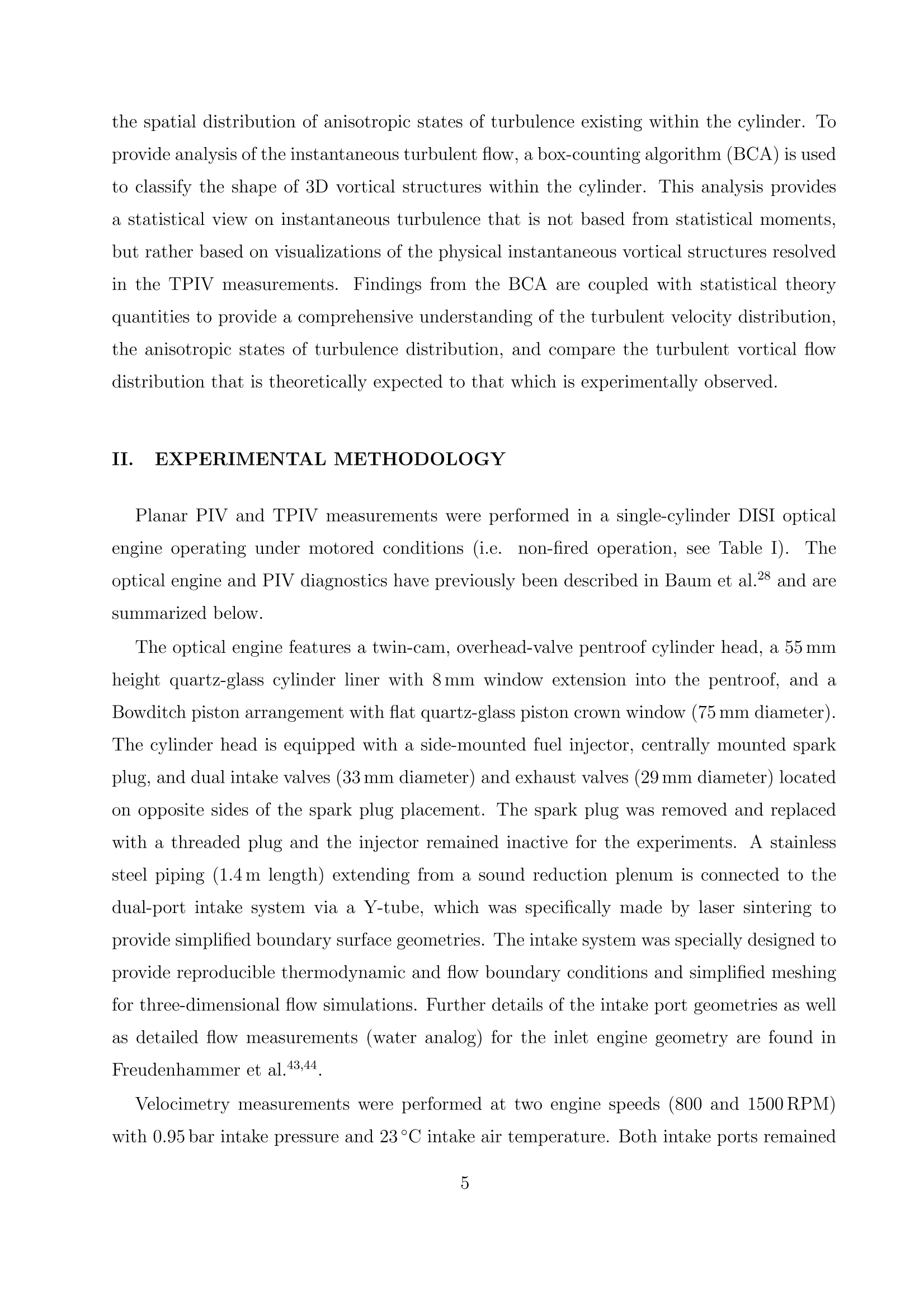
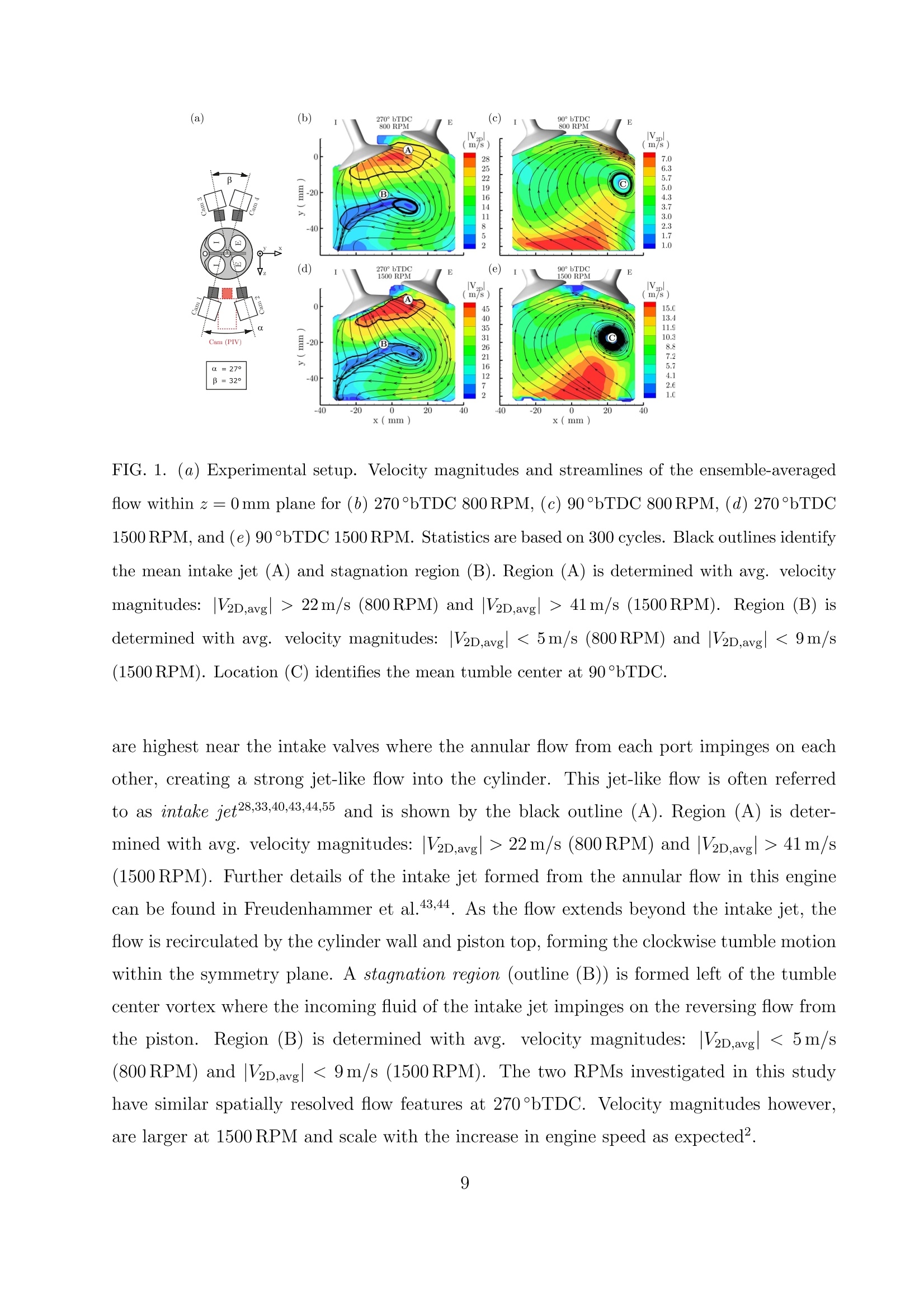
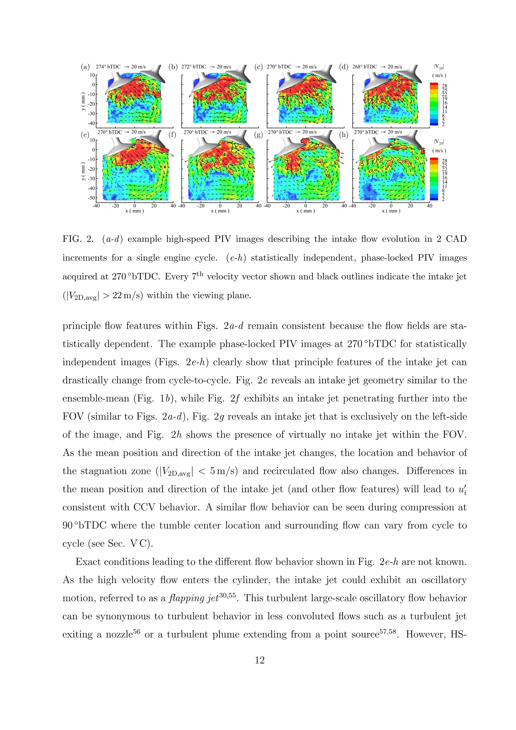
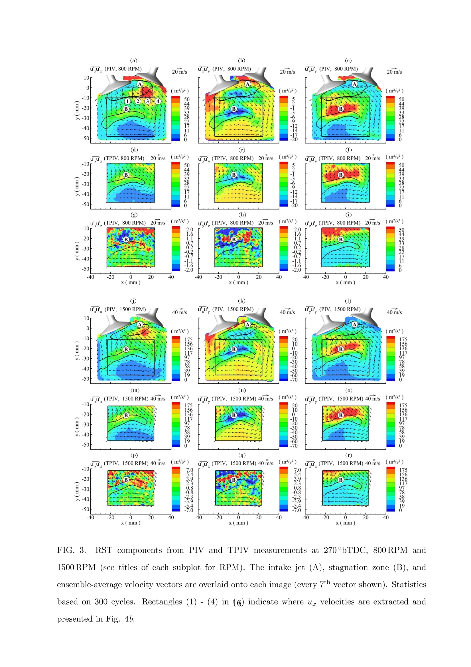
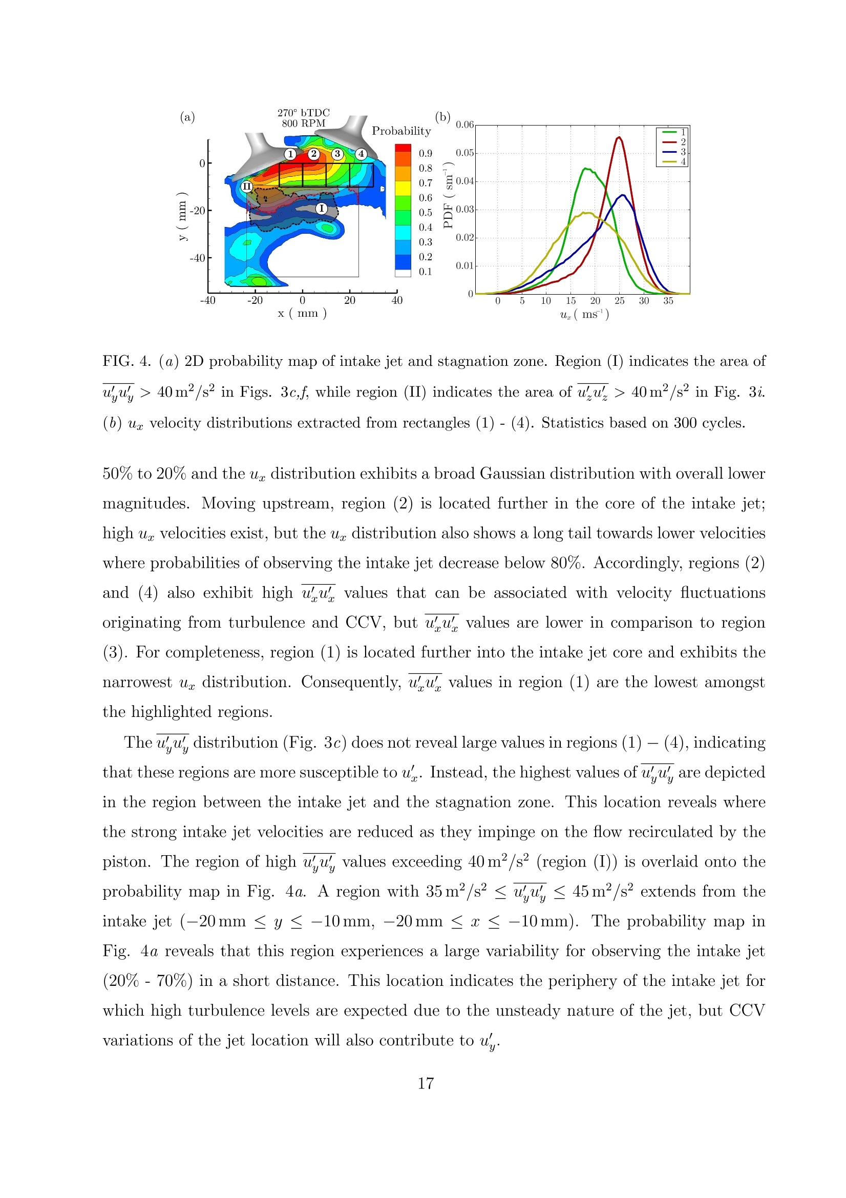
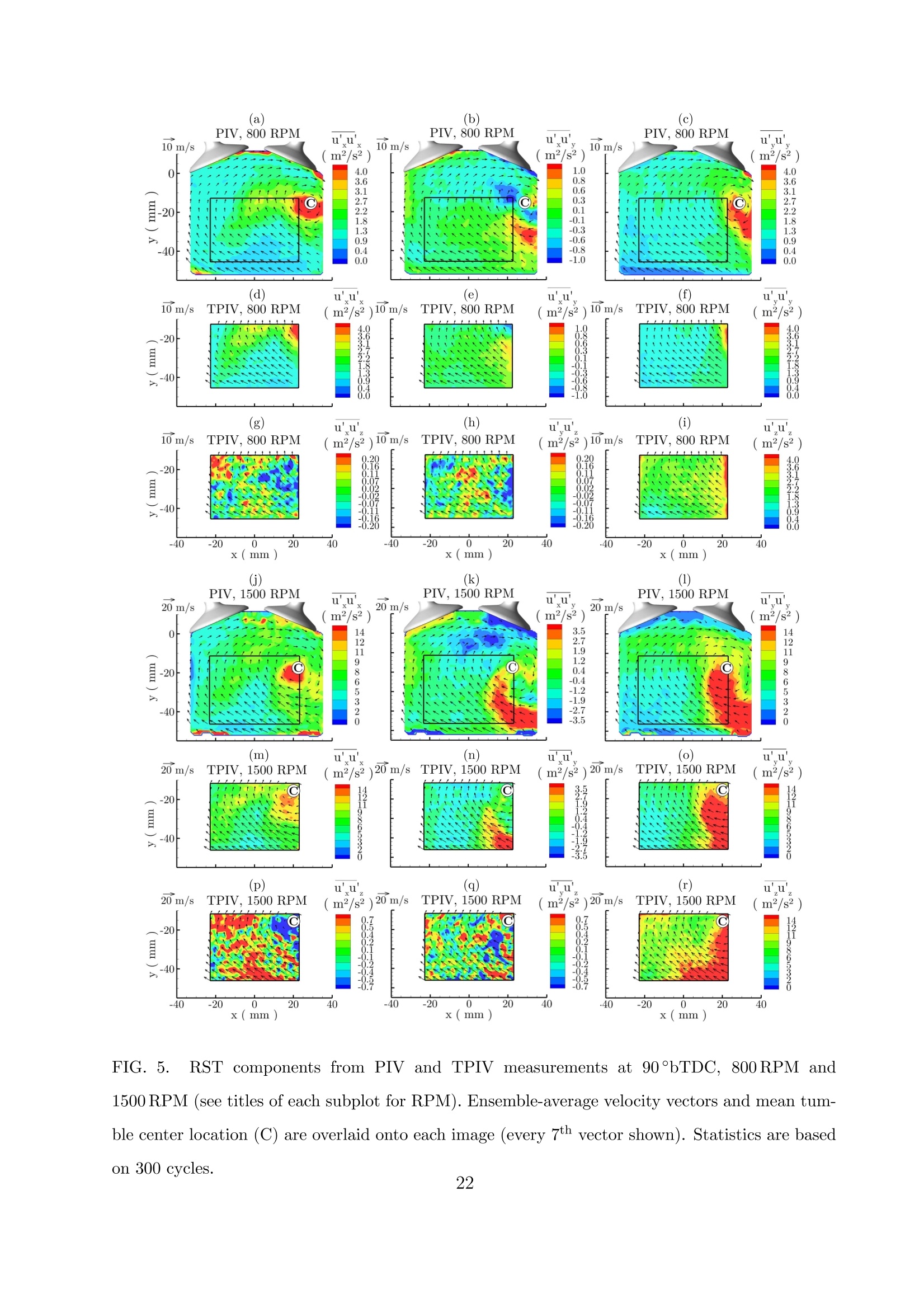
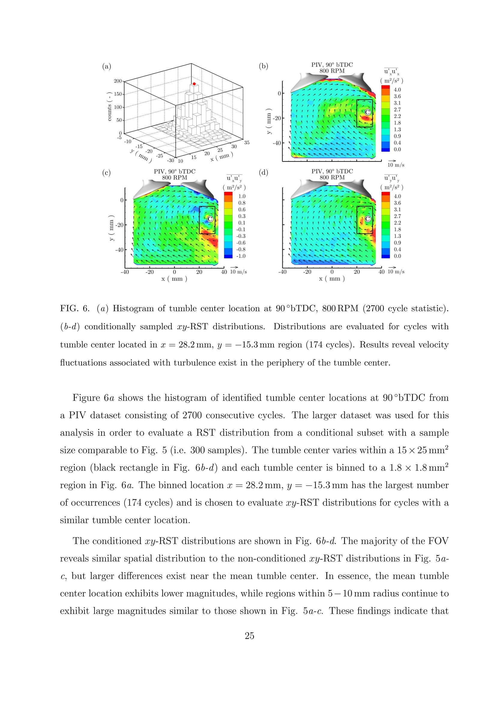

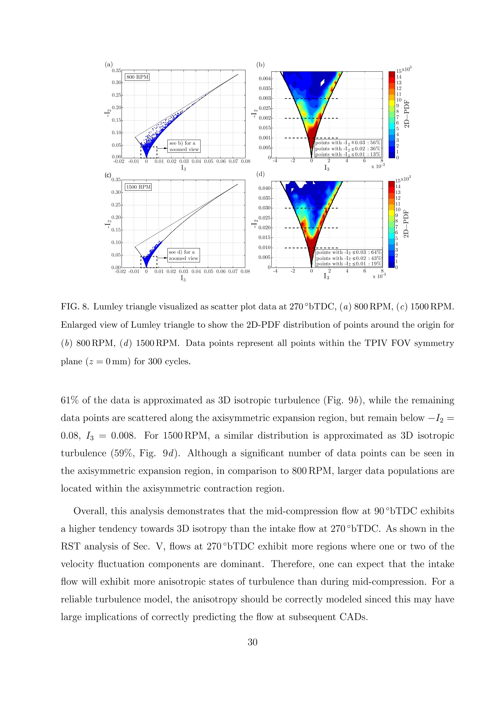
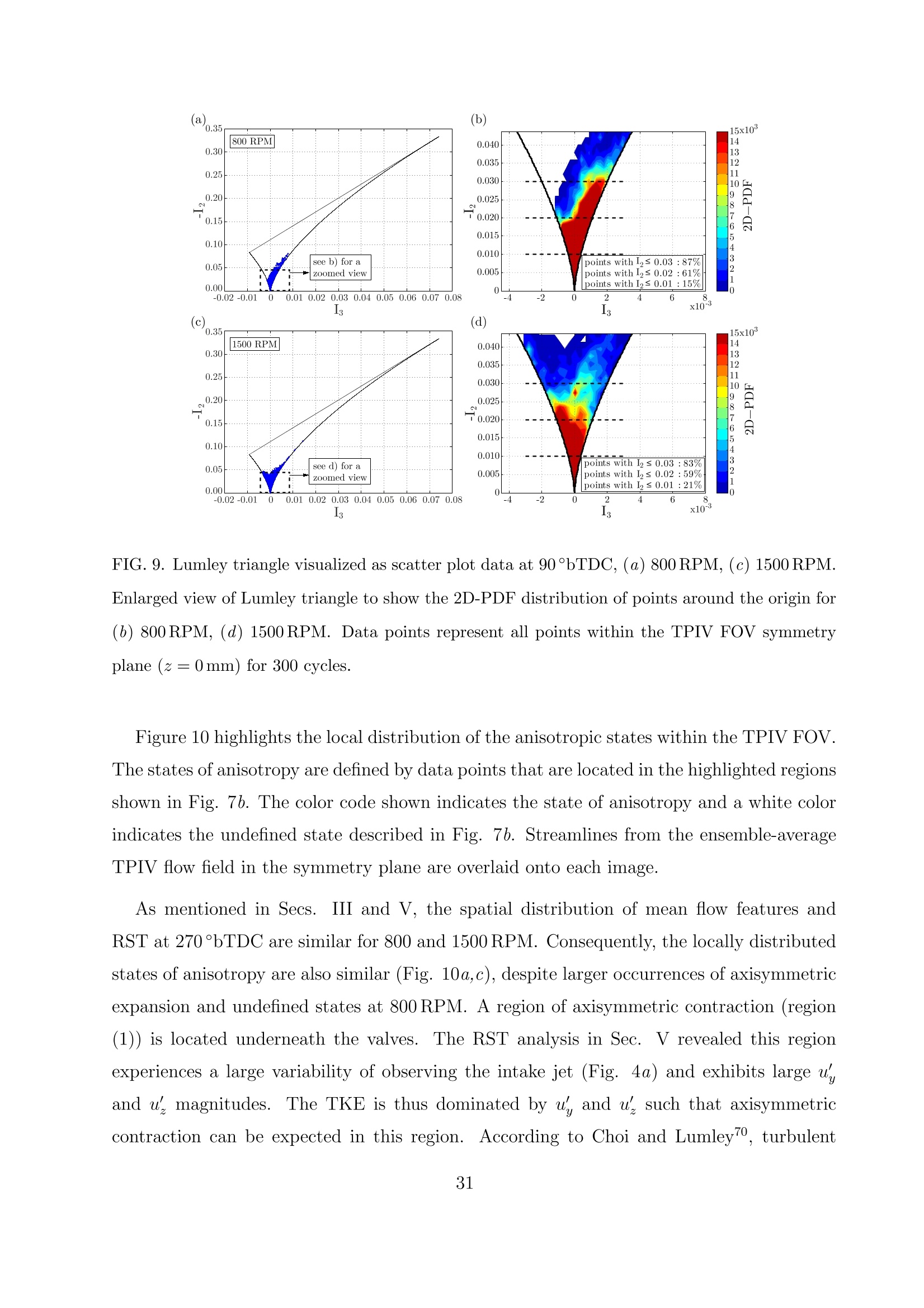
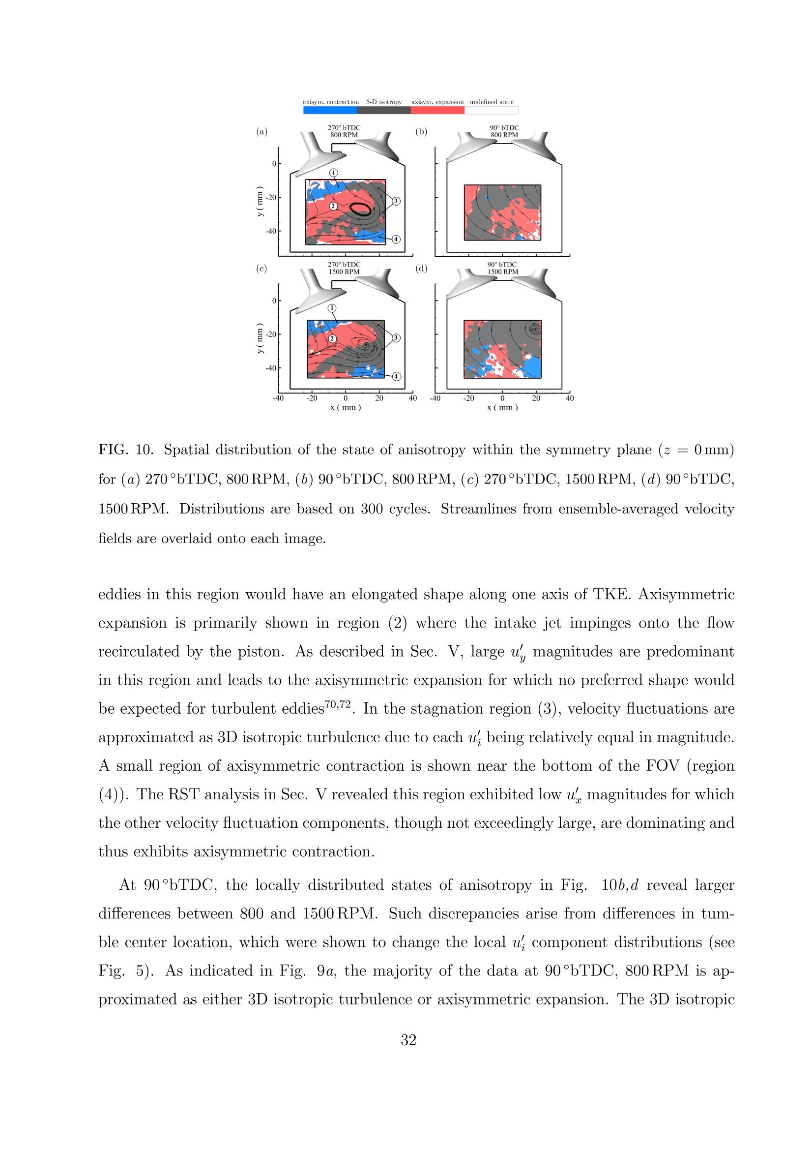
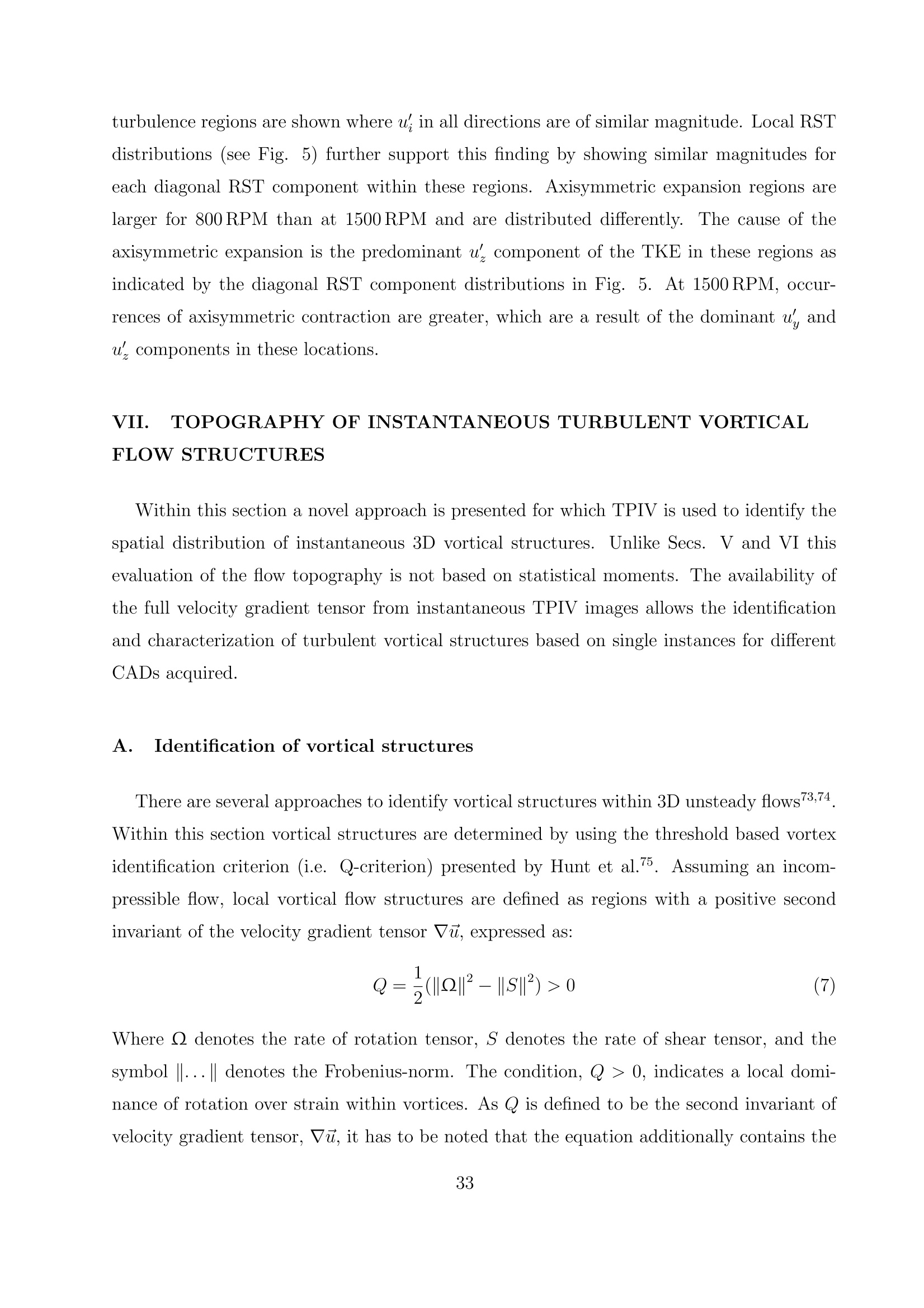

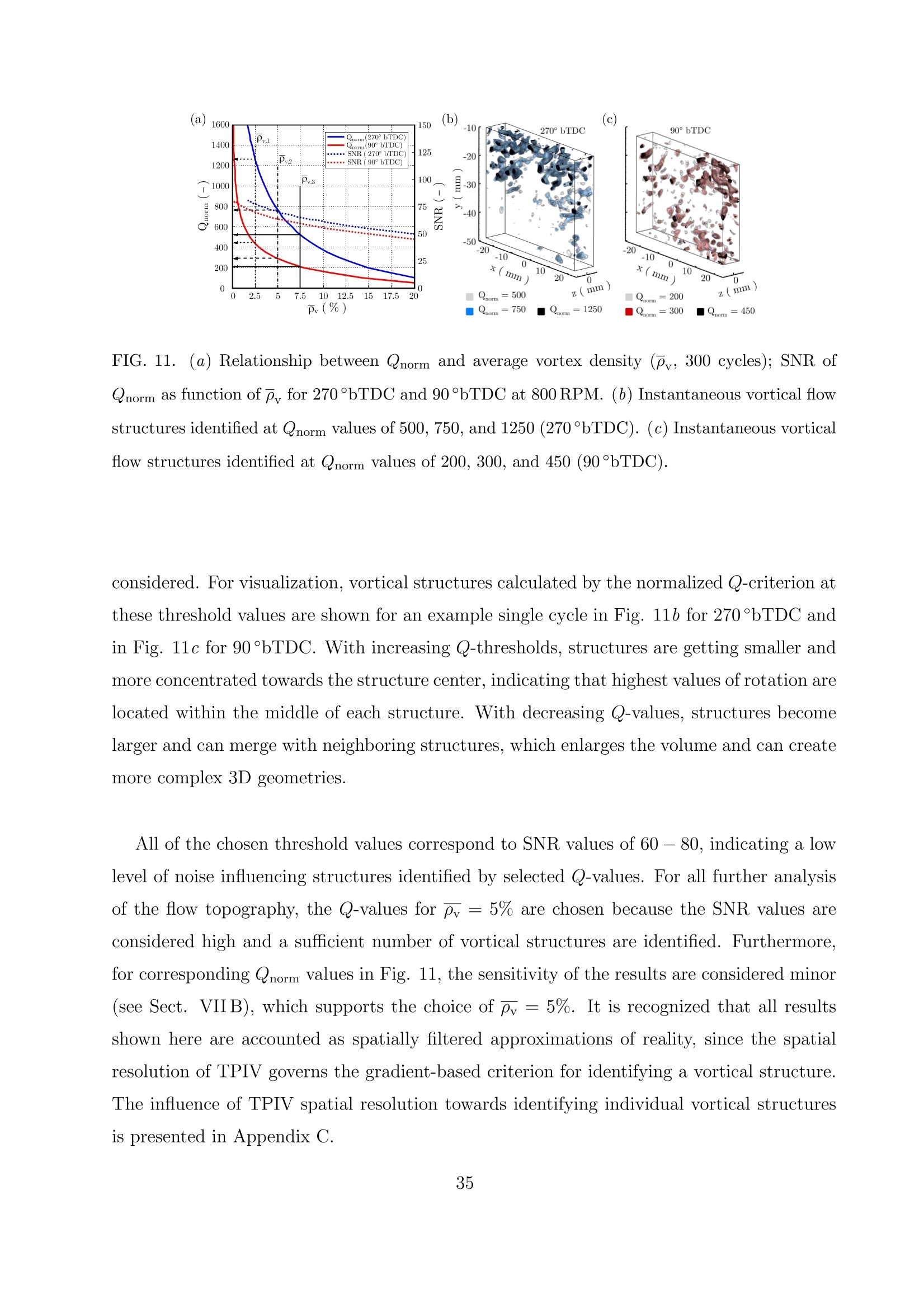
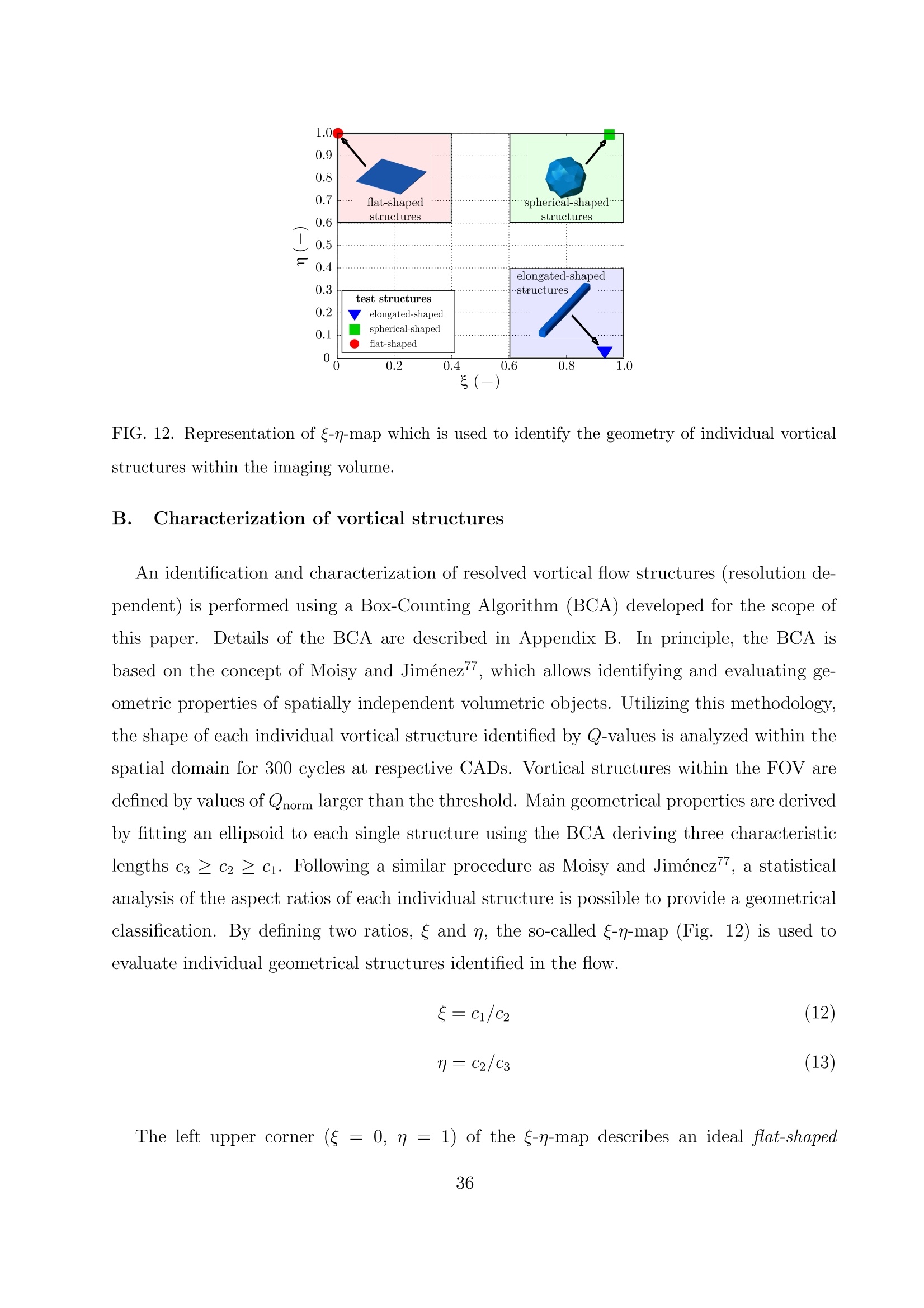
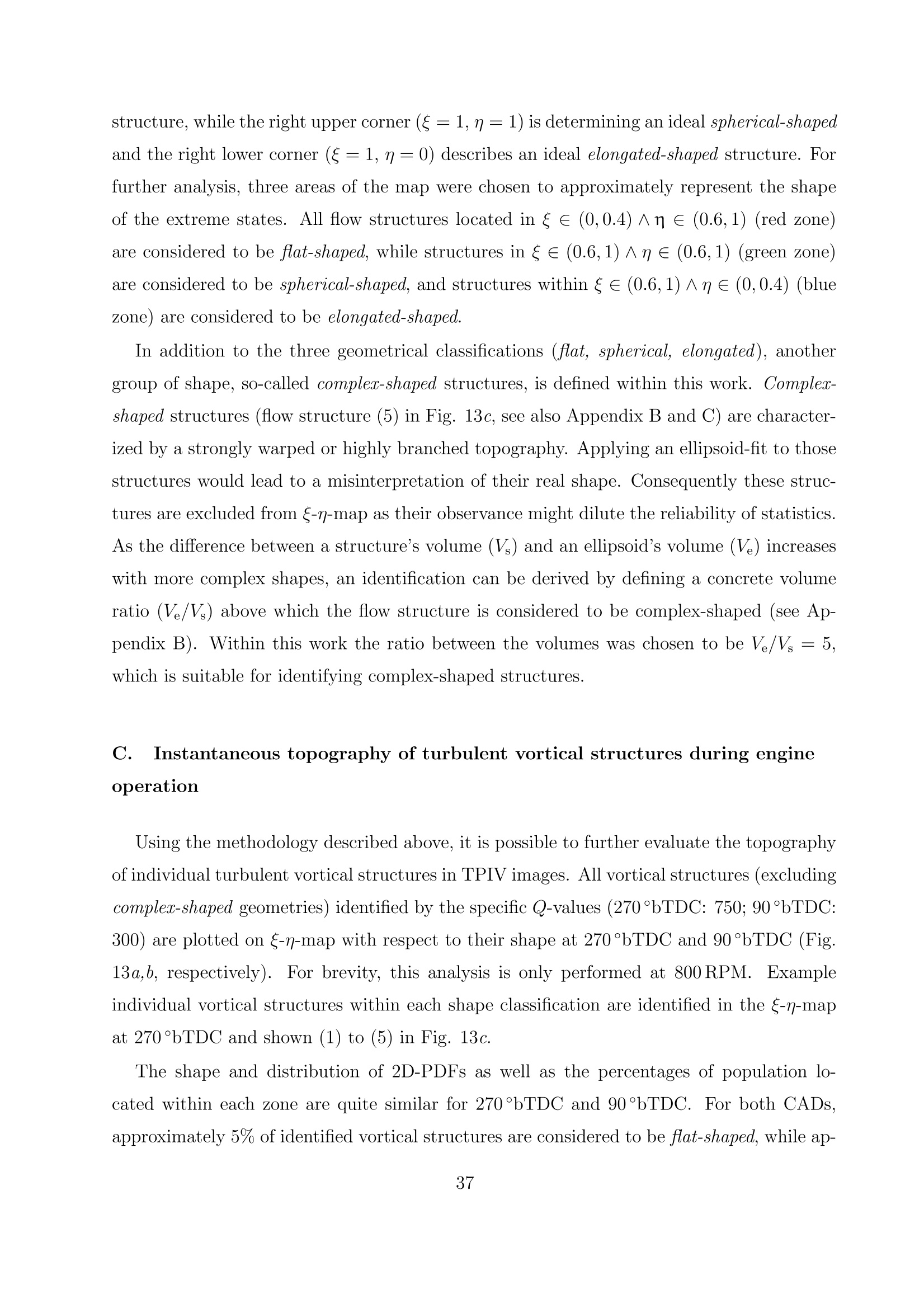
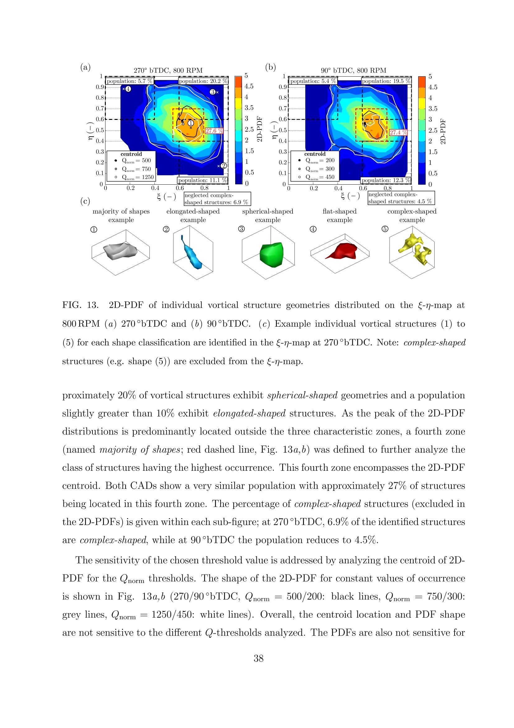
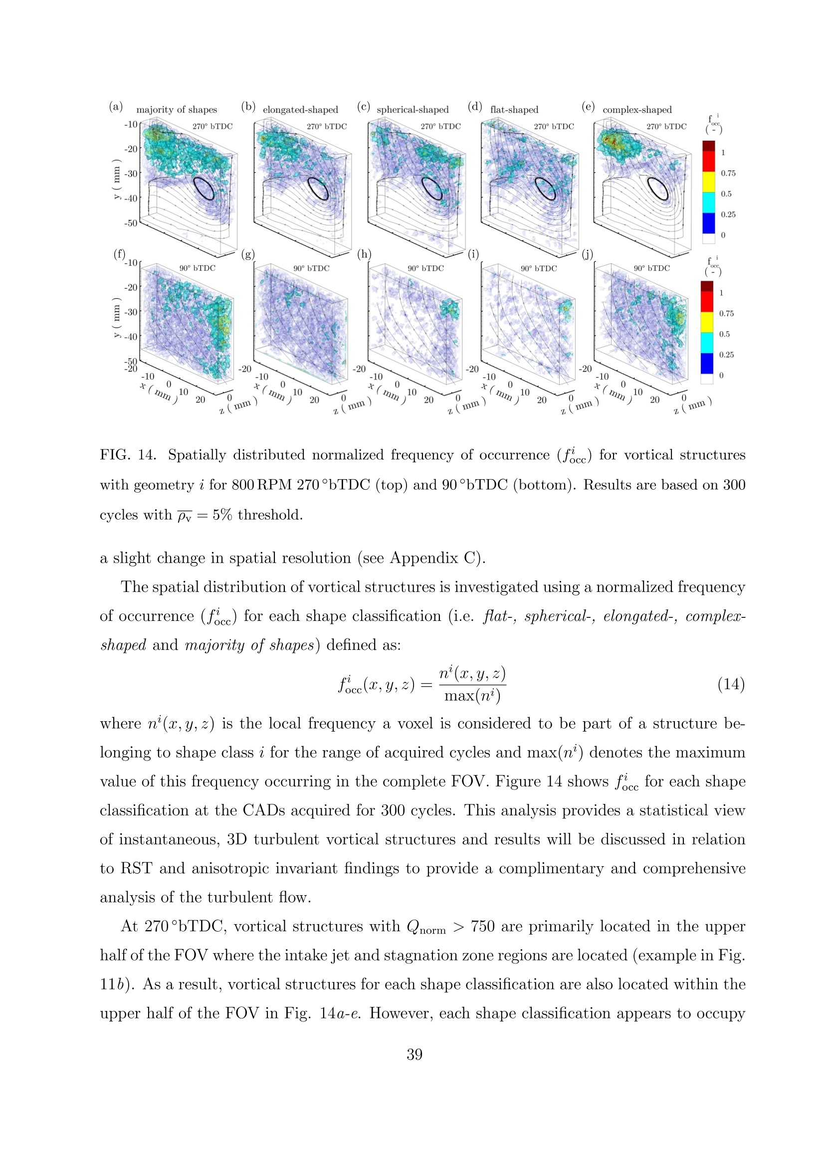
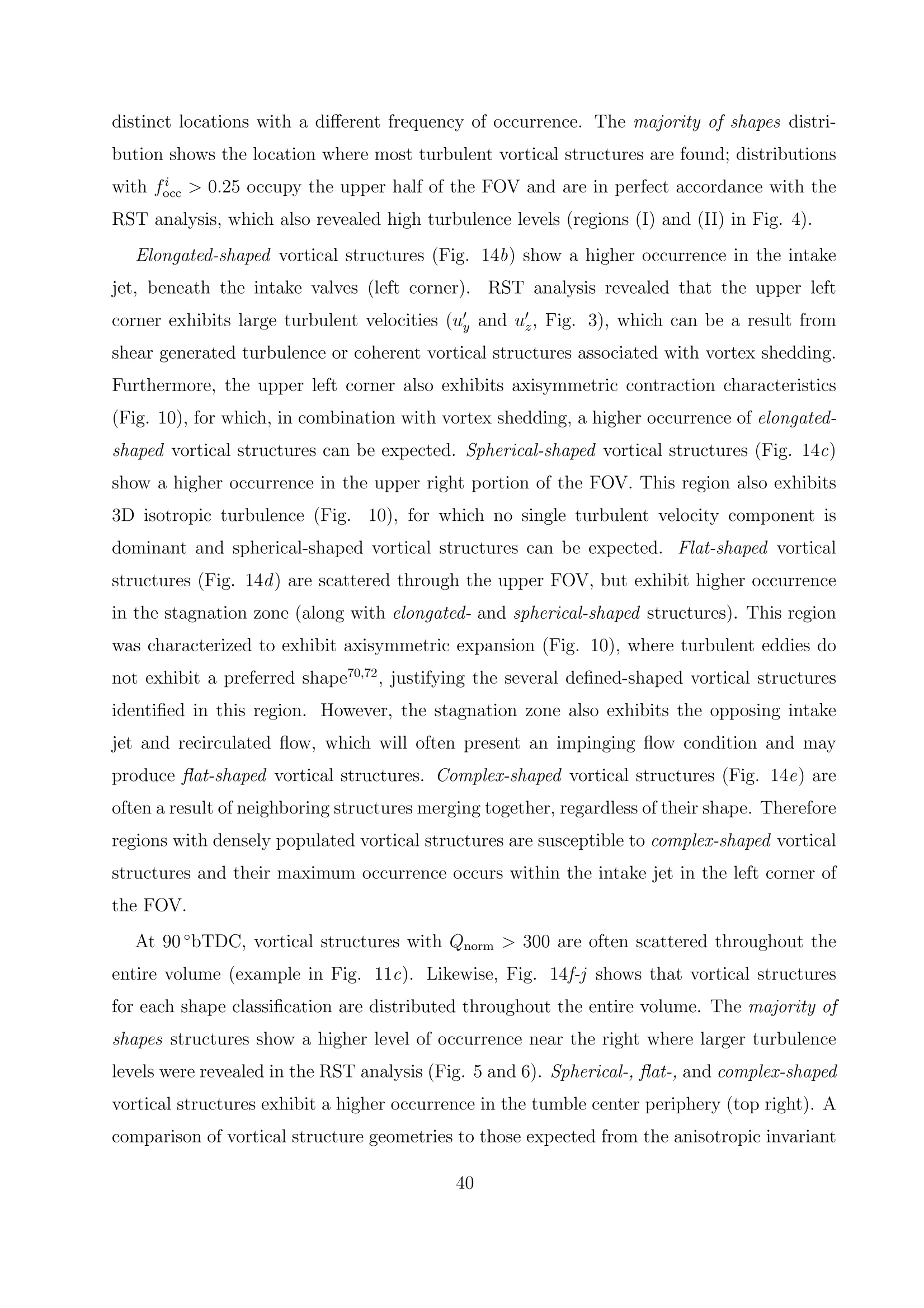

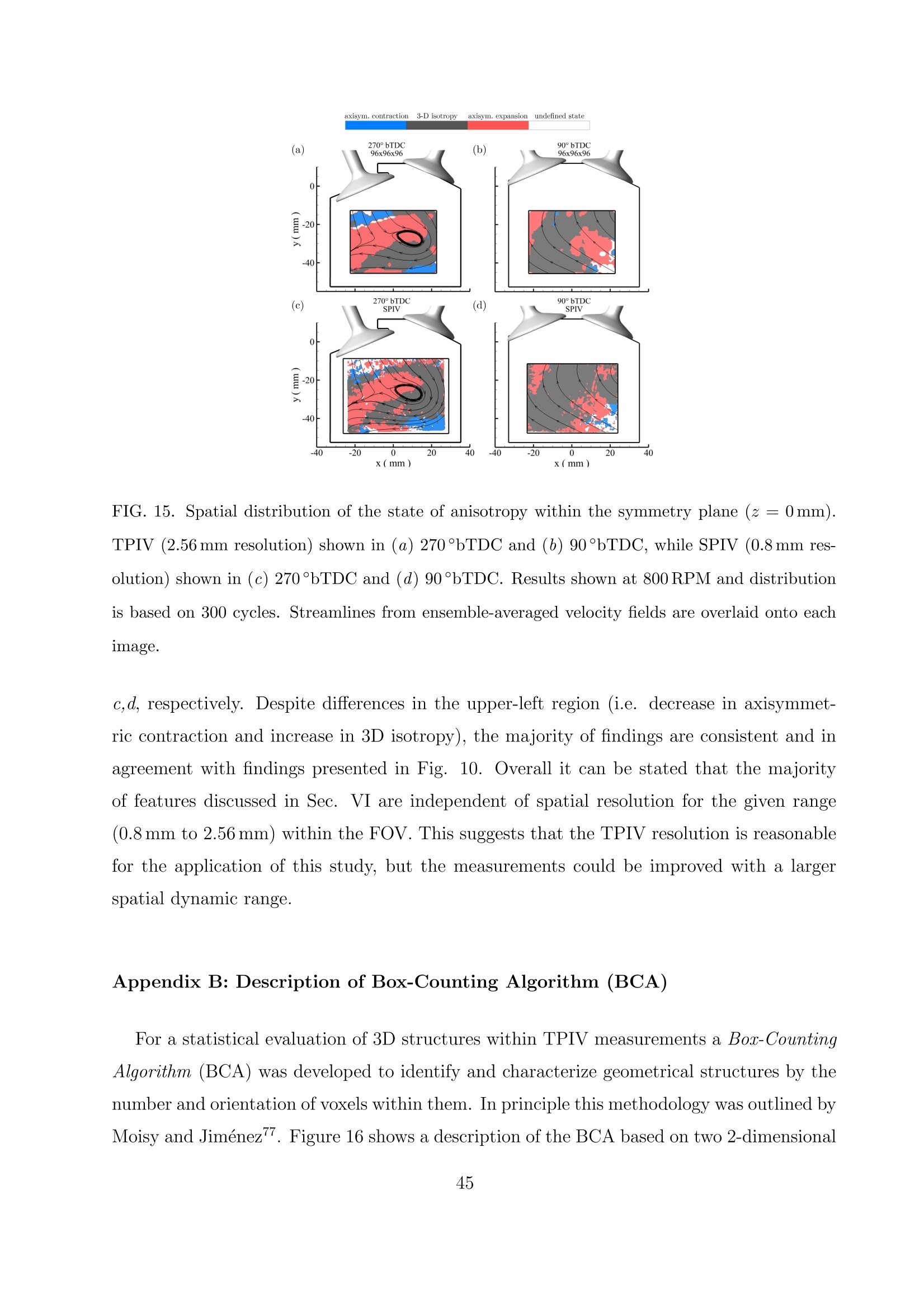
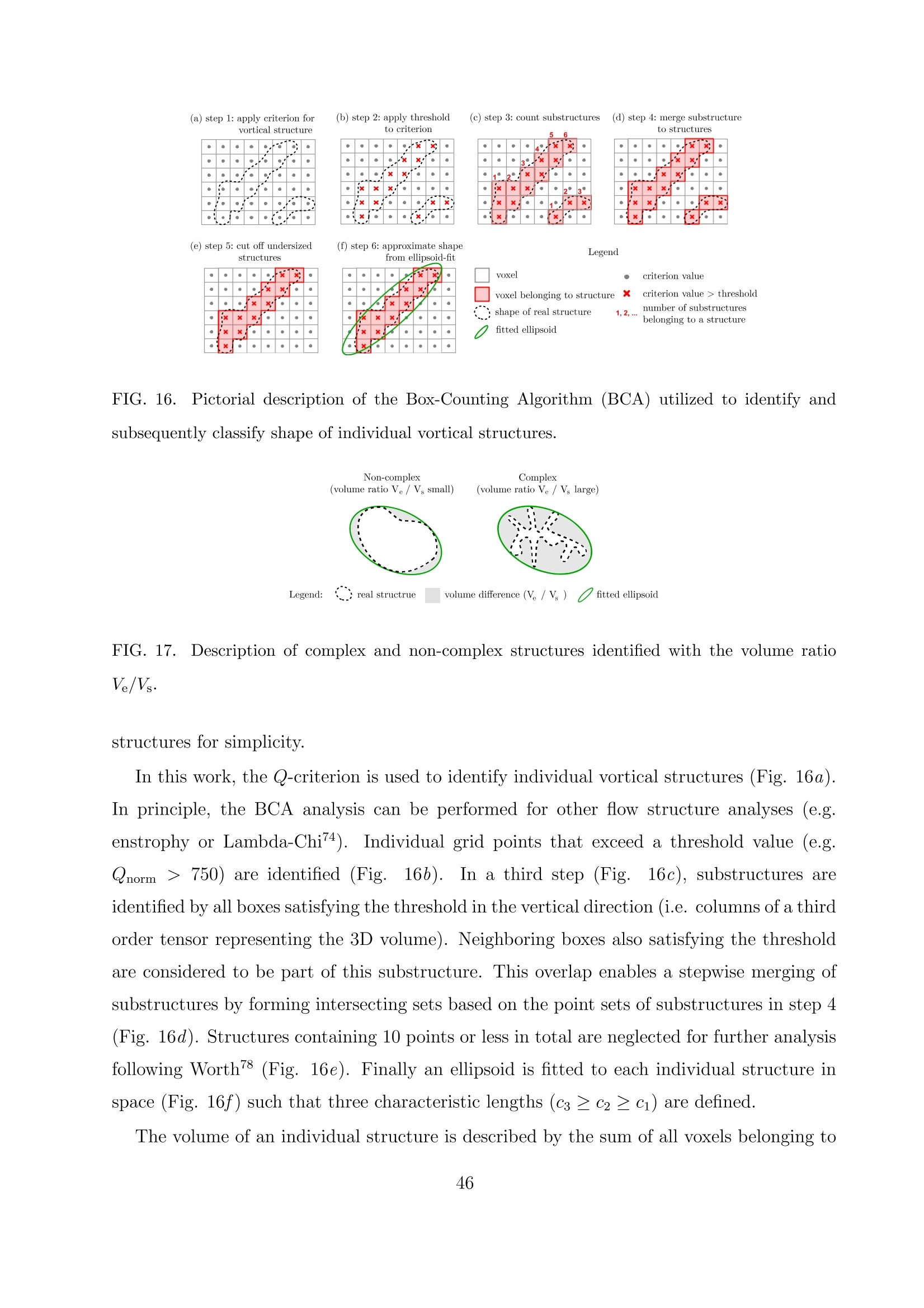
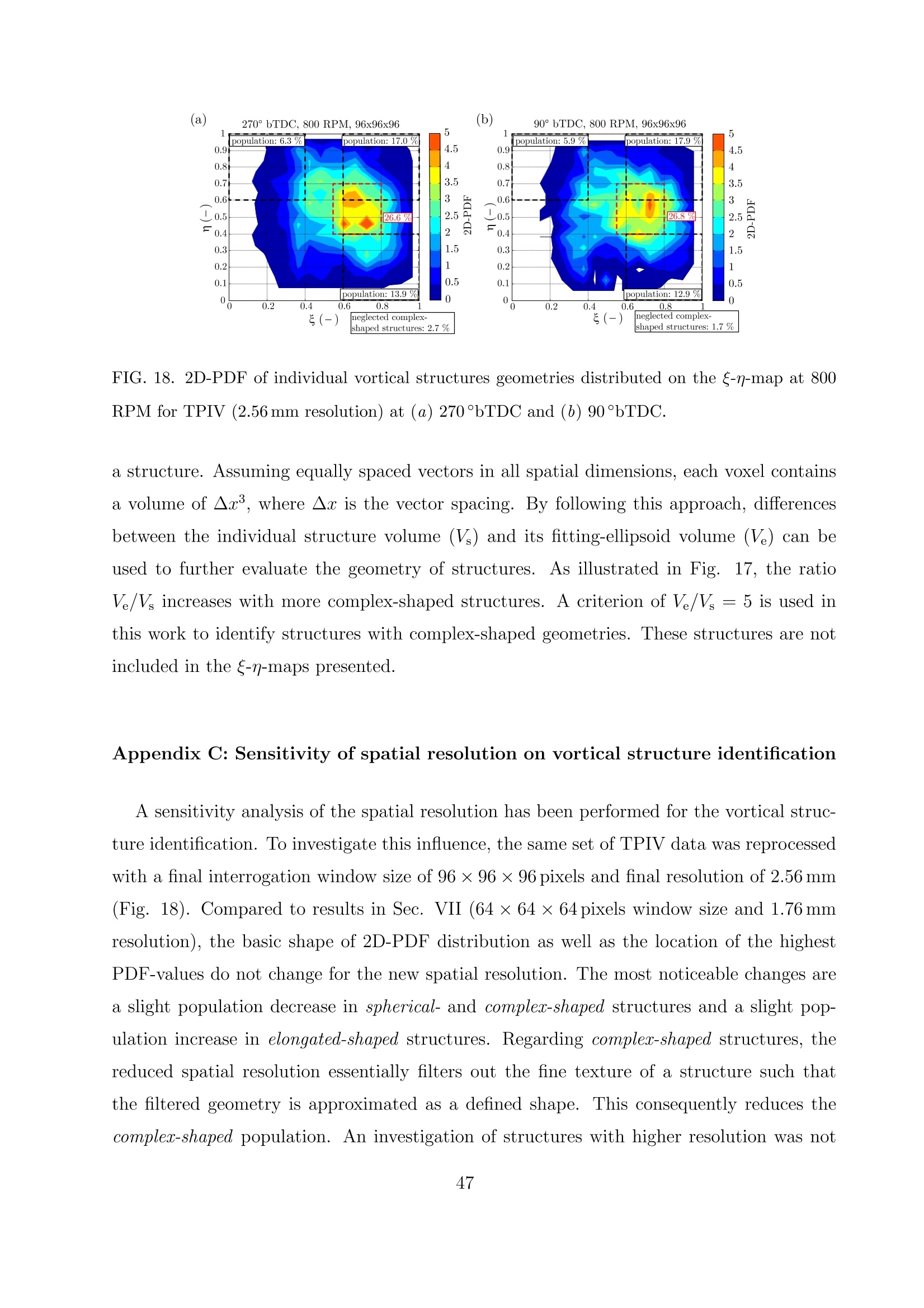


还剩54页未读,是否继续阅读?

产品配置单

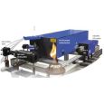
北京欧兰科技发展有限公司为您提供《发动机内流场中速度场,涡量场检测方案(粒子图像测速)》,该方案主要用于汽车电子电器中其他检测,参考标准--,《发动机内流场中速度场,涡量场检测方案(粒子图像测速)》用到的仪器有体视层析粒子成像测速系统(Tomo-PIV)、时间分辨平面激光诱导荧光测量系统
推荐专场


相关方案
更多
该厂商其他方案
更多