


方案详情
文
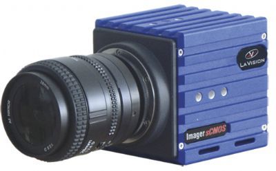
采用LaVision公司由4台sCMOS型相机和DaVis8.2软件平台构成的大视场2D2C粒子成像测速系统,对破漏层模型的流程进行了初步的实验分析。
方案详情

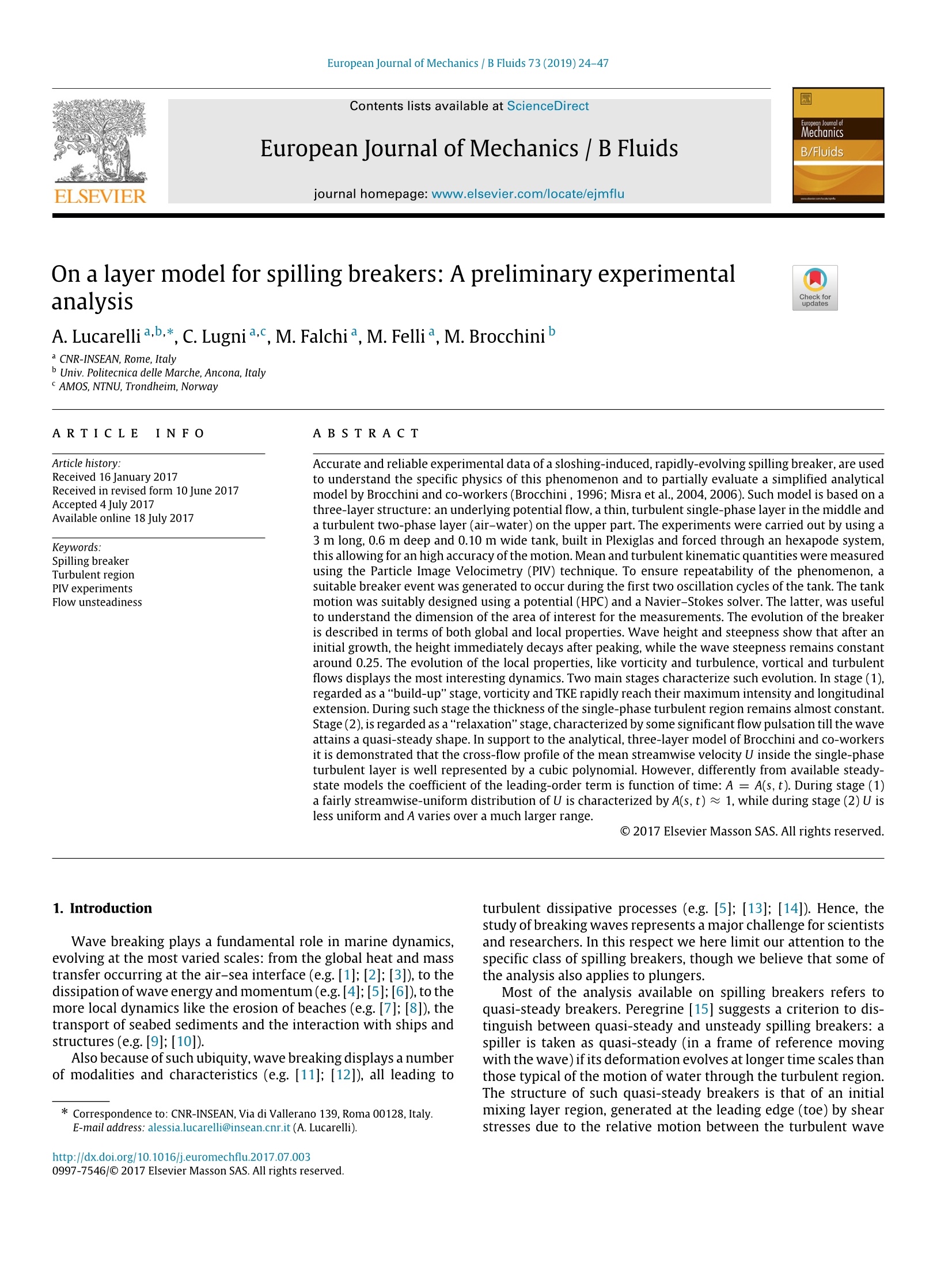
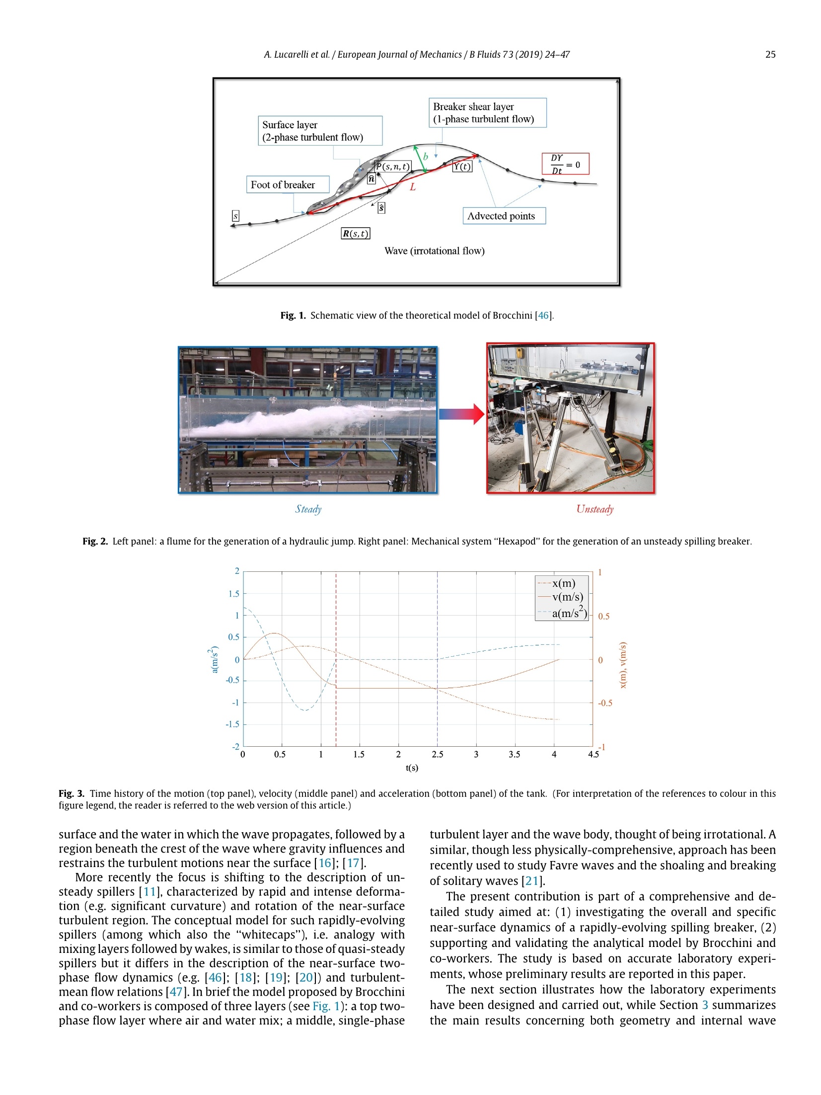
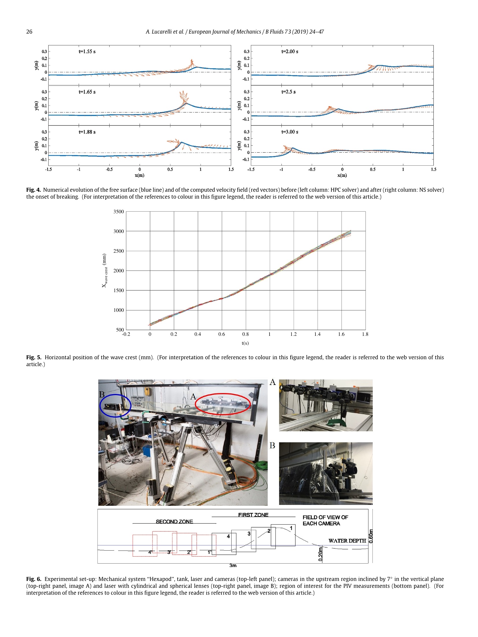
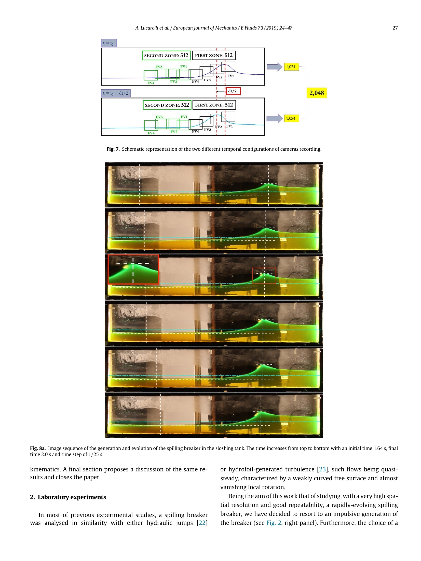
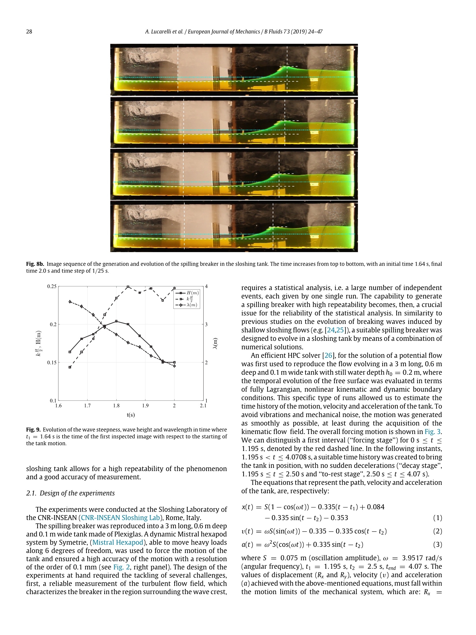
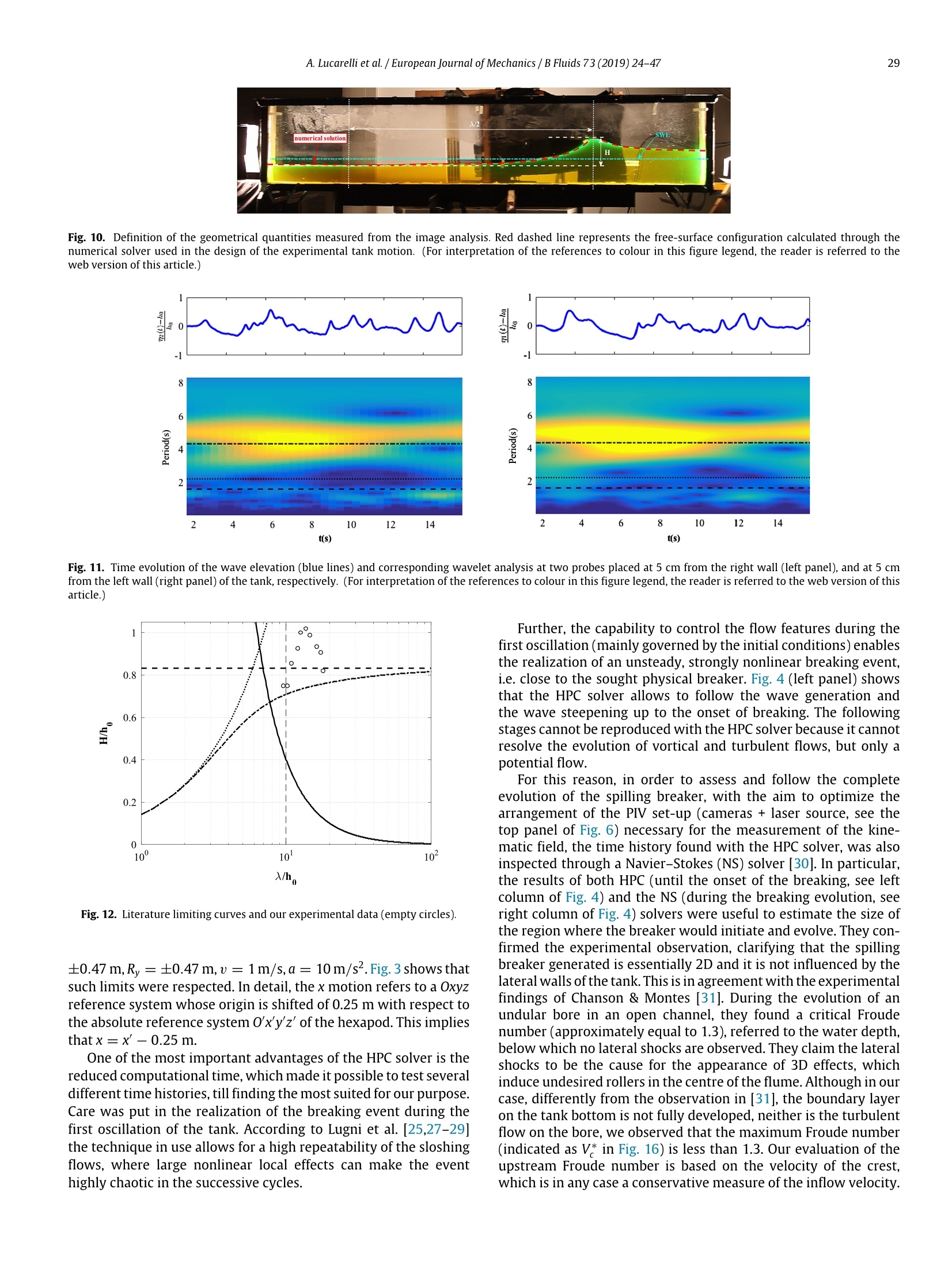
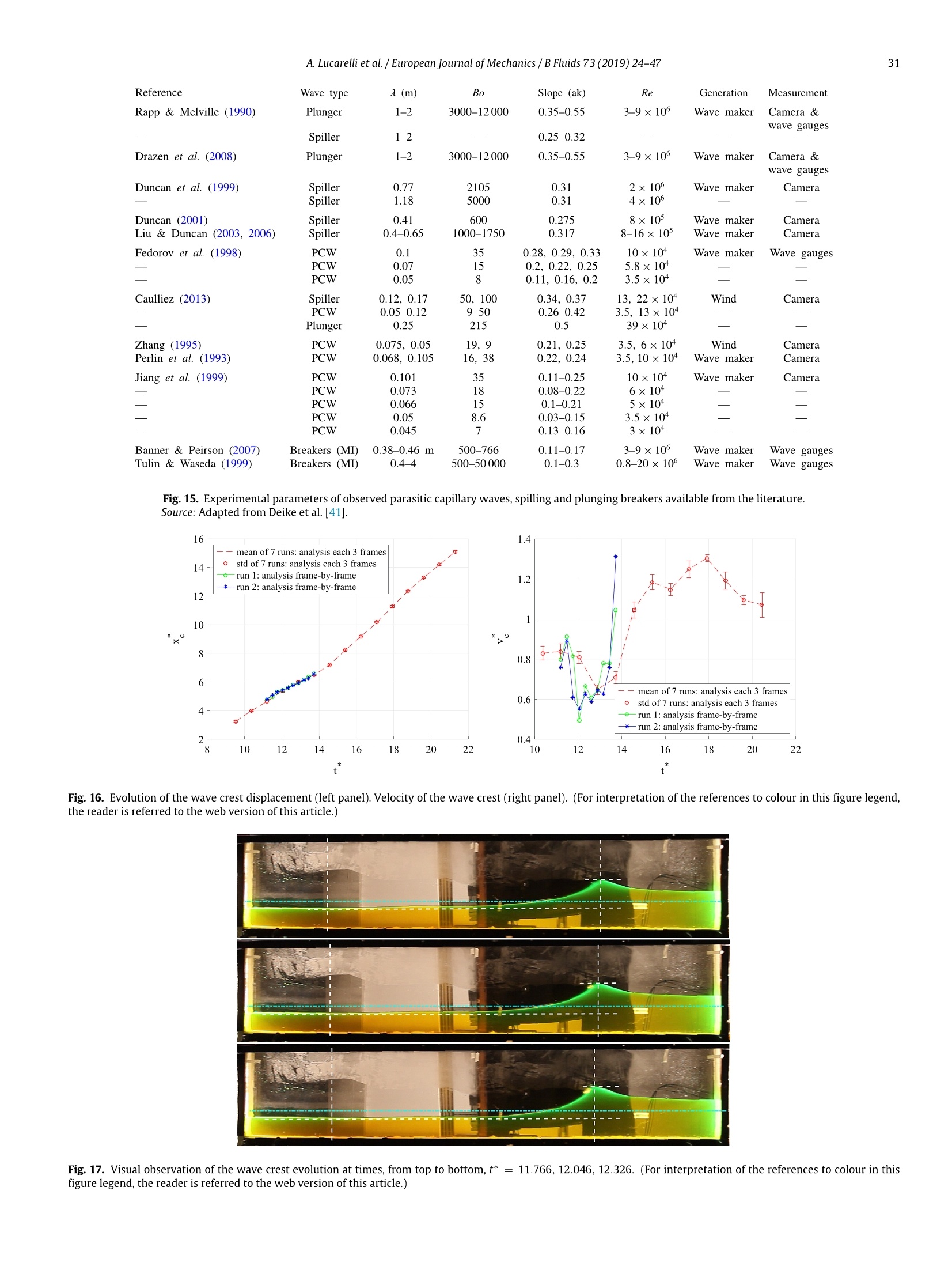
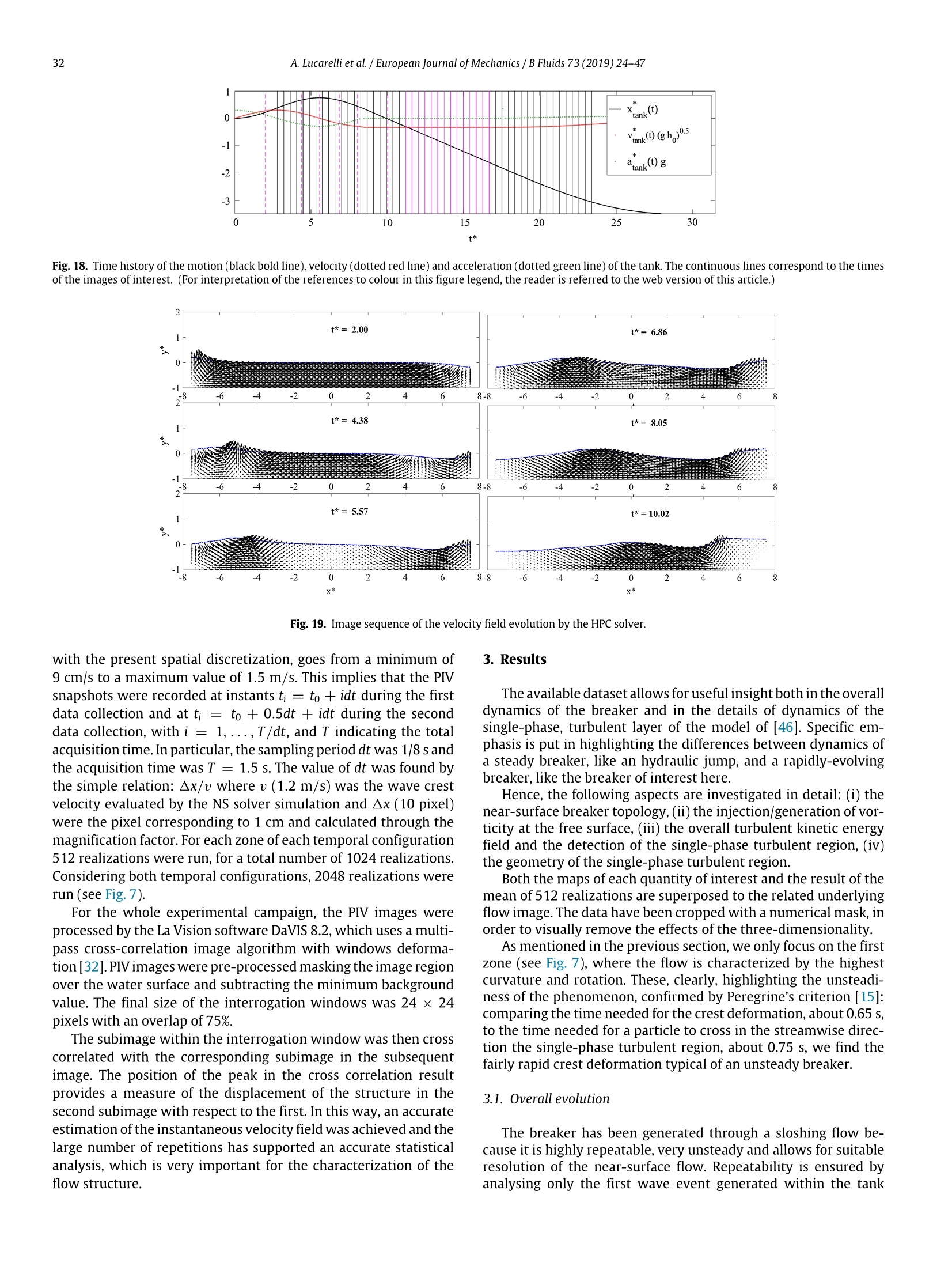
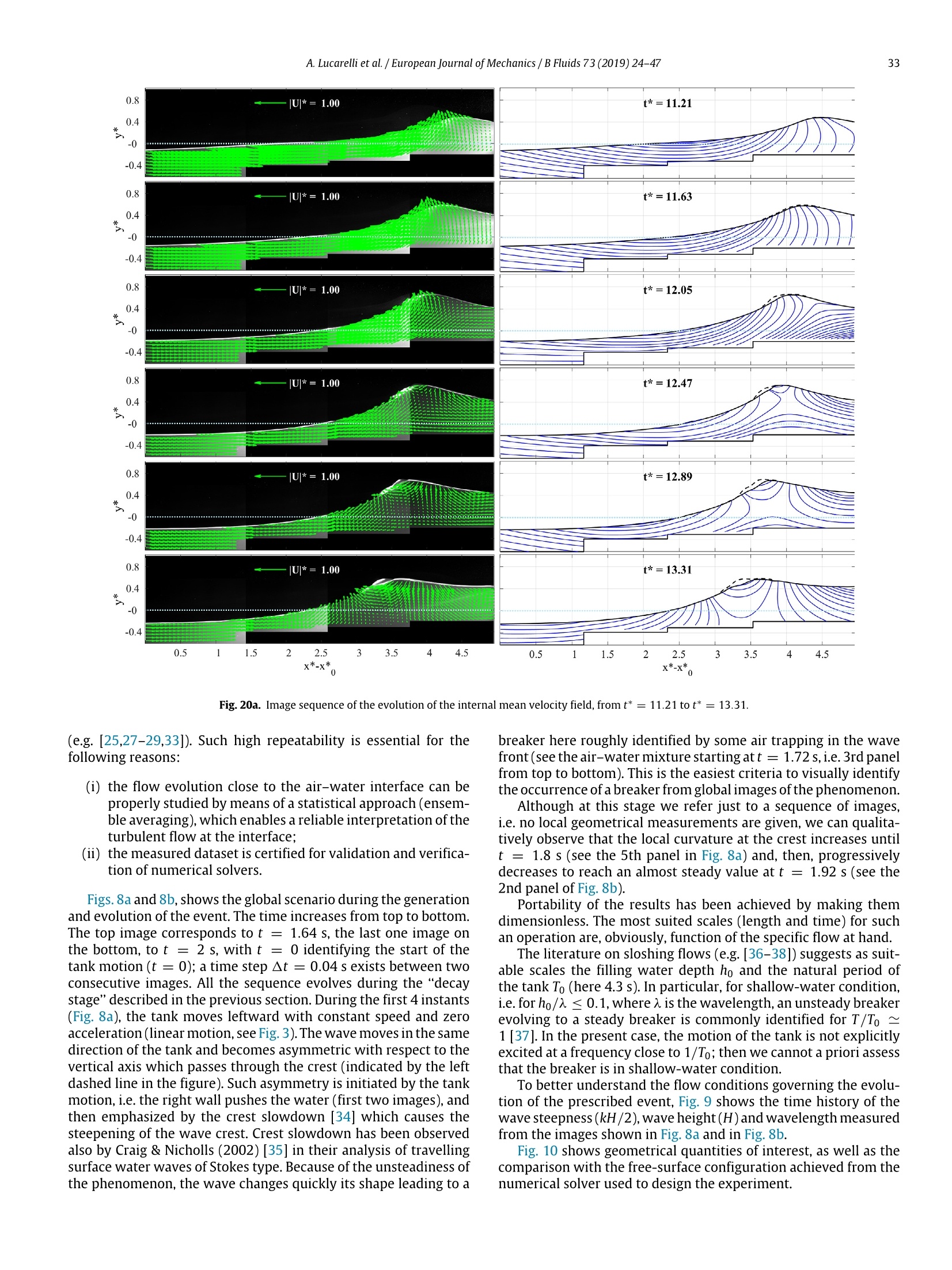
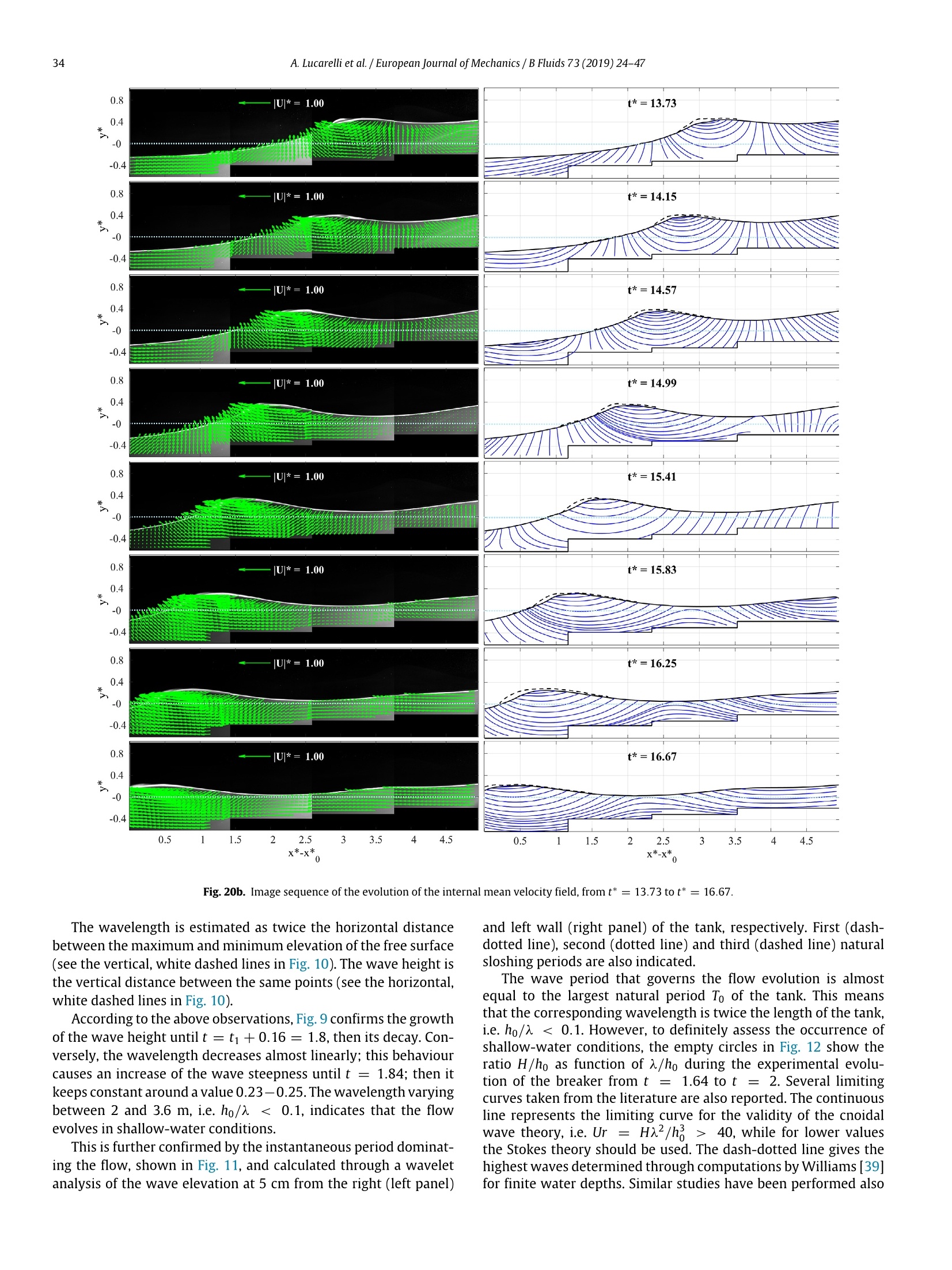
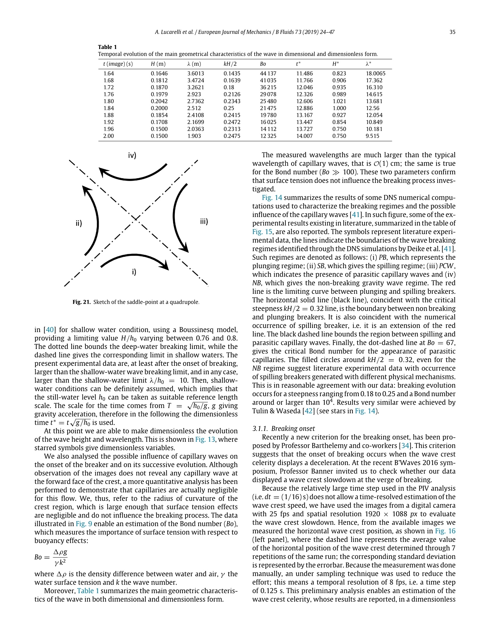
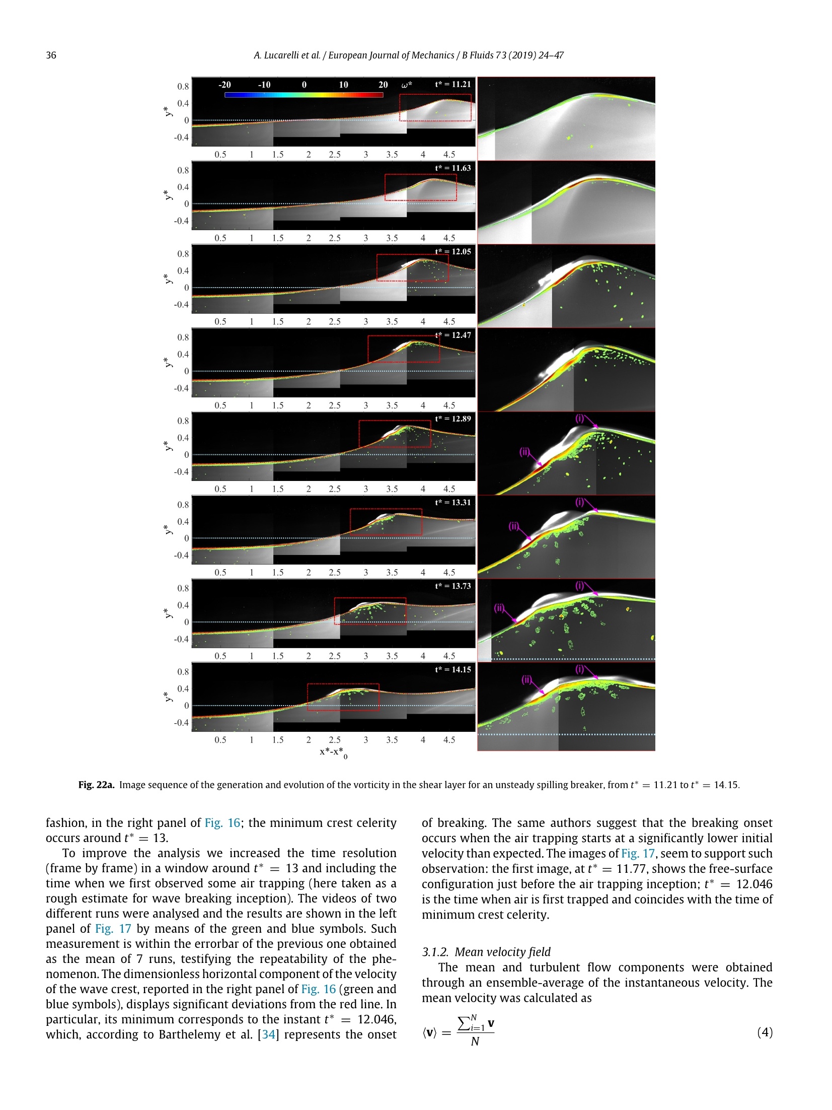
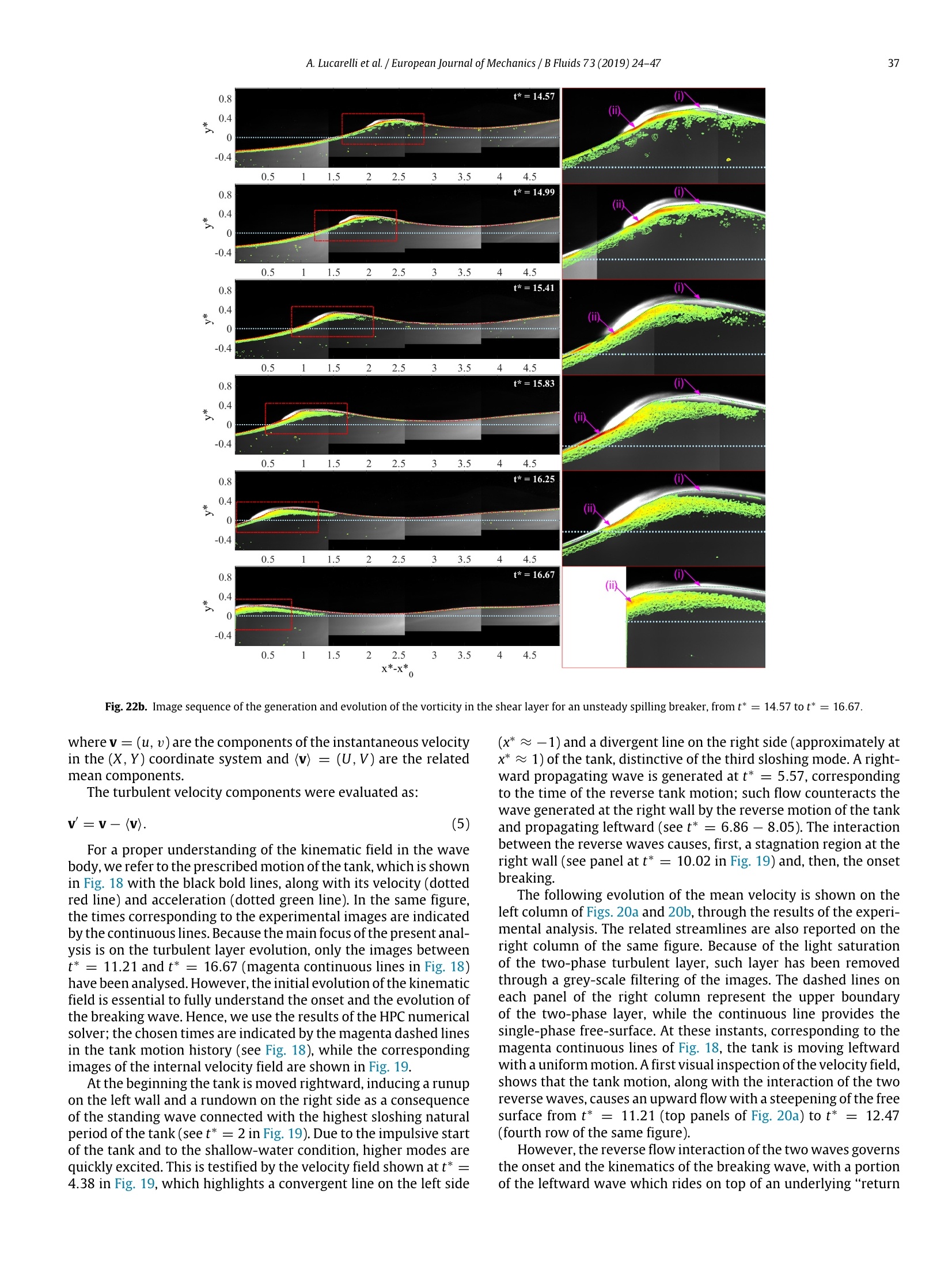
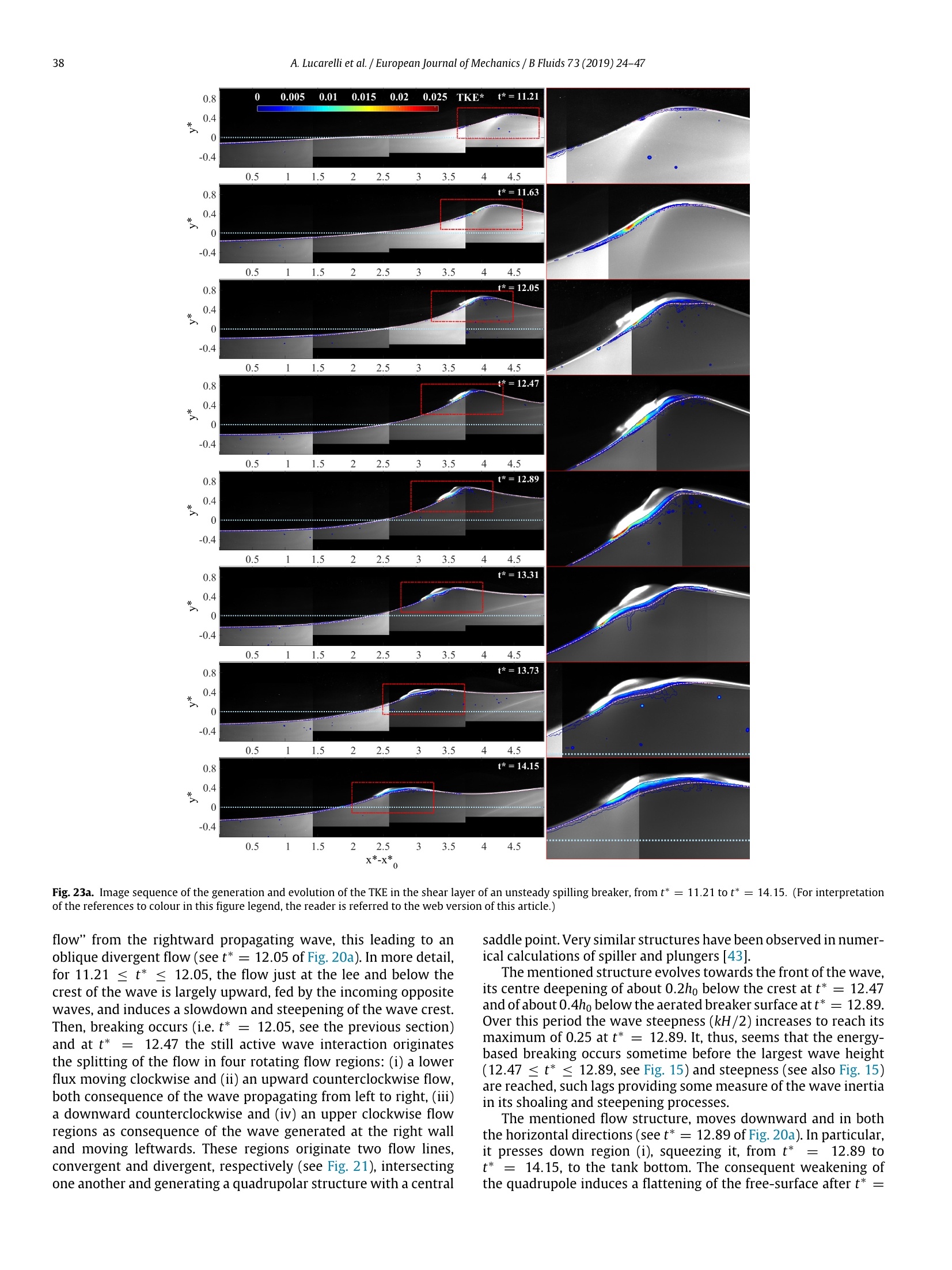
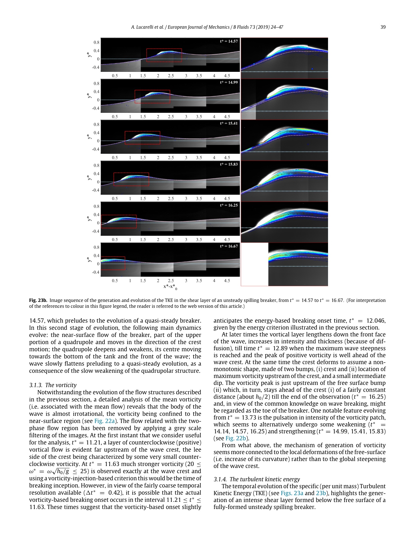
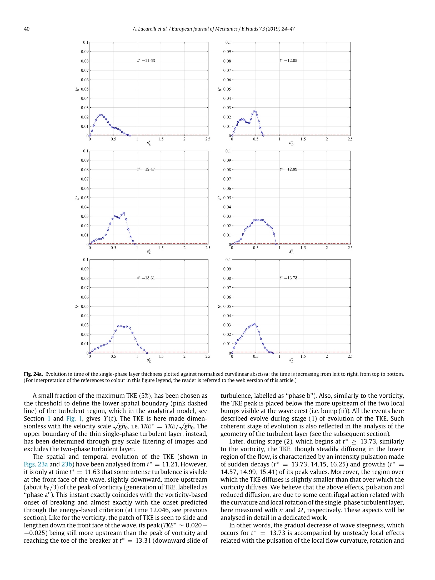
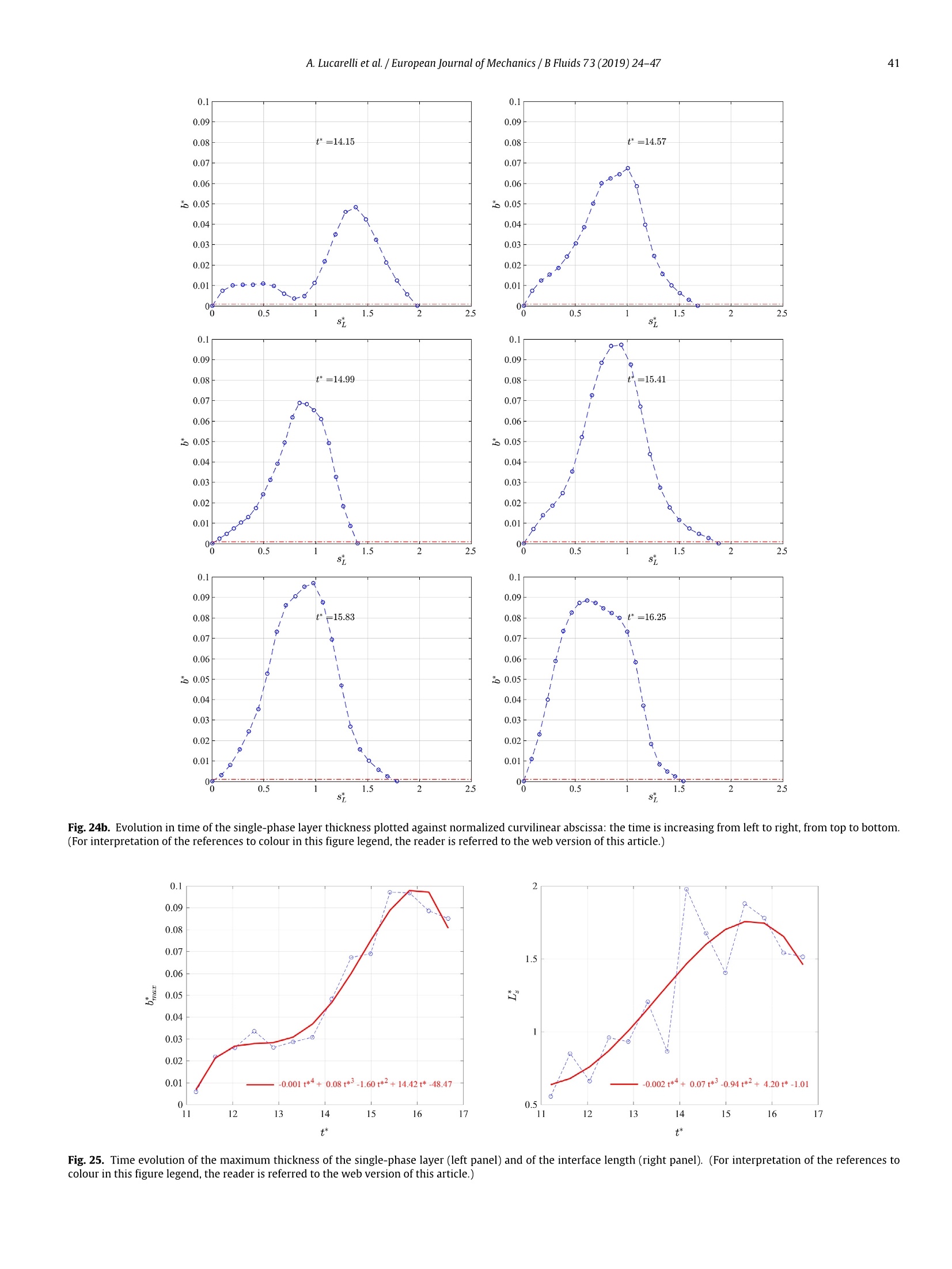
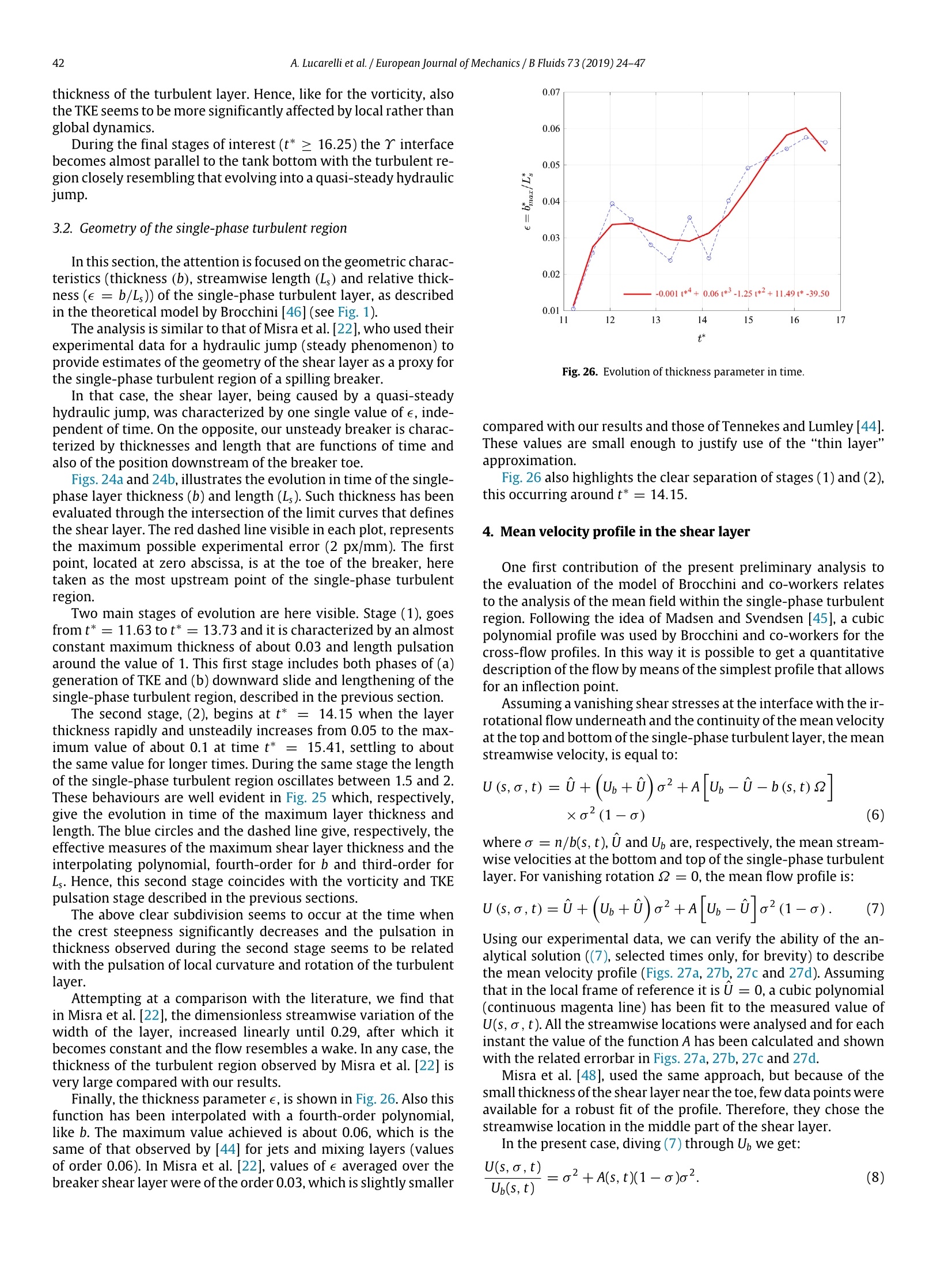
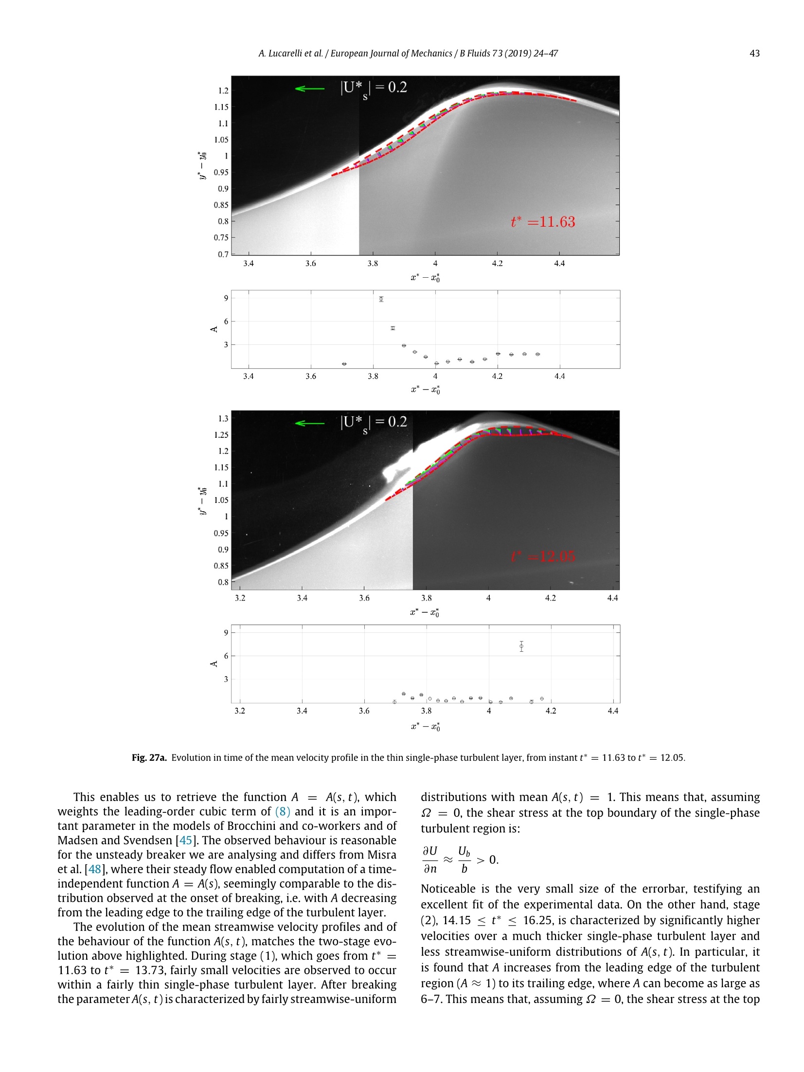
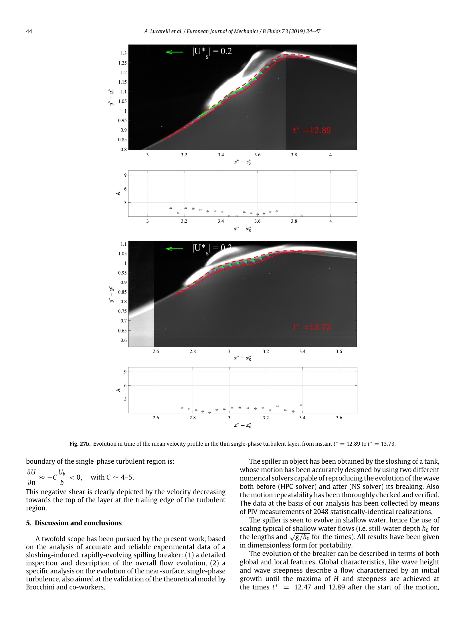
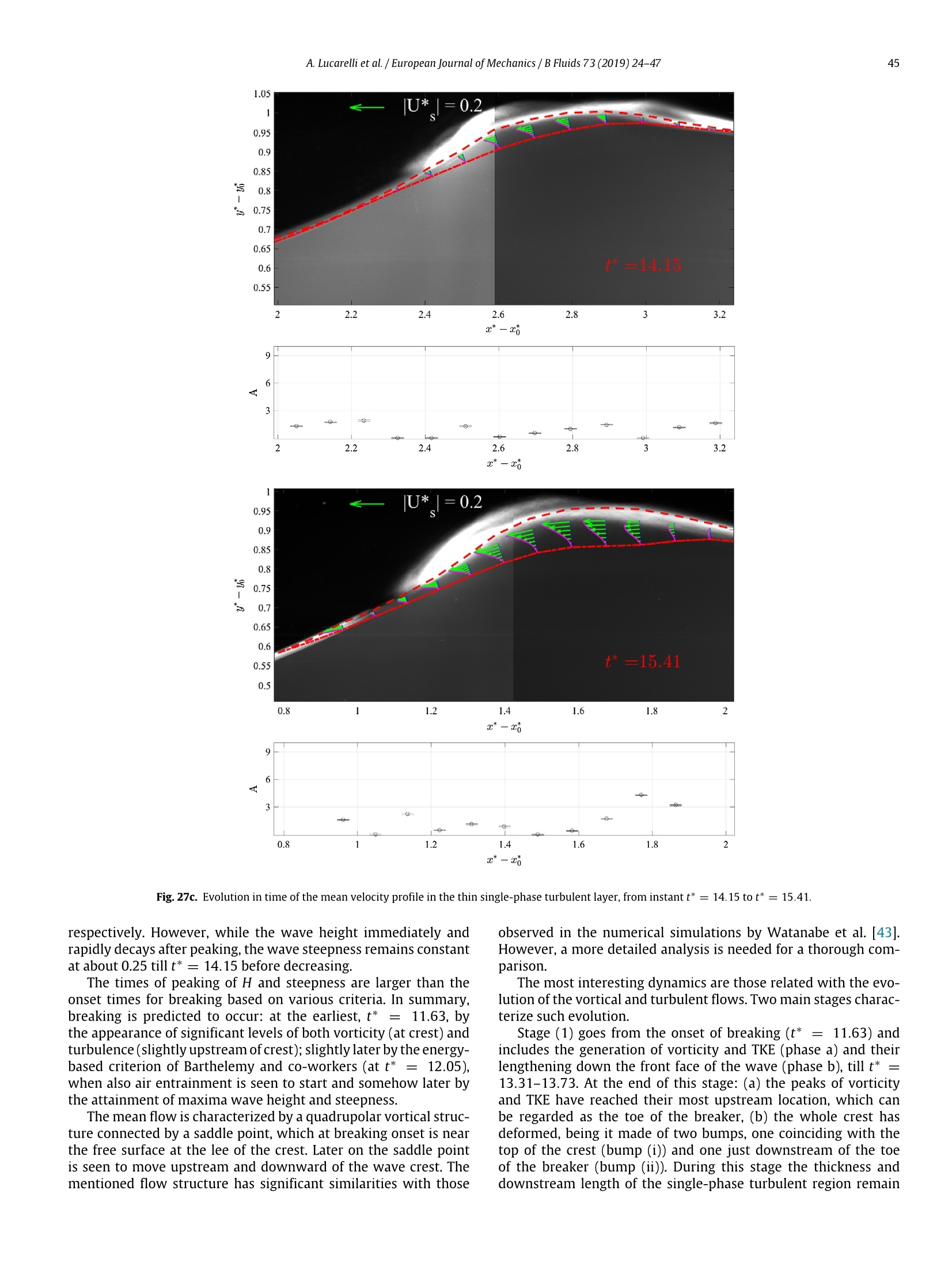
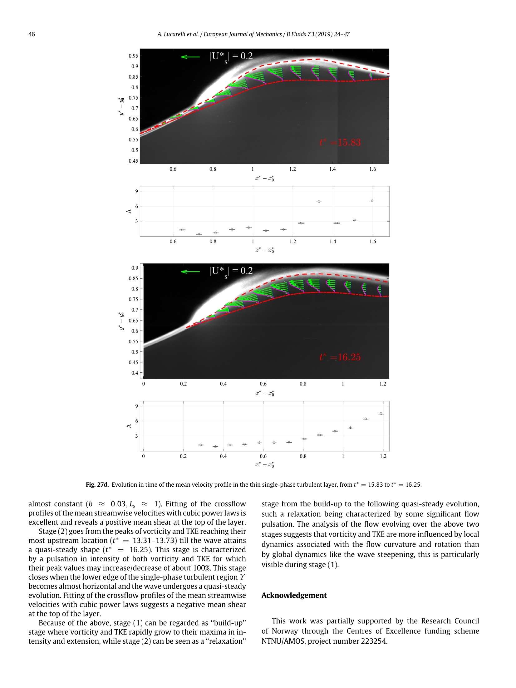
European Journal of Mechanics /B Fluids 73 (2019)24-47 A. Lucarelli et al. / European Journal of Mechanics / B Fluids 73 (2019) 24-4725 Contents lists available at ScienceDirect European Journal of Mechanics /B Fluids ELSEVIER journal homepage: www.elsevier.com/locate/ejmflu On a layer model for spilling breakers: A preliminary experimentalanalysis A. Lucarellia,b,*, C. Lugni.c,M. Falchi, M. Felli, M. BrocchiniCNR-INSEAN, Rome, ItalyUniv. Politecnica delle Marche, Ancona, Italy‘ AMOS, NTNU, Trondheim, Norway ARTICLE I N F O ABSTR A C T Article history:Received 16 January 2017Received in revised form 10 June 2017Accepted 4 July 2017 Available online 18 July 2017 Accurate and reliable experimental data of a sloshing-induced,rapidly-evolving spilling breaker, are usedto understand the specific physics of this phenomenon and to partially evaluate a simplified analyticalmodel by Brocchini and co-workers (Brocchini, 1996; Misra et al.,2004,2006). Such model is based on athree-layer structure: an underlying potential flow, a thin, turbulent single-phase layer in the middle anda turbulent two-phase layer (air-water) on the upper part. The experiments were carried out by using a3K m long, 0.6 m deep andeywords: 0.10 m wide tank, built in Plexiglas and forced through an hexapode system,Spilling breakerthis allowing for an high accuracy ofthe motion. Mean and turbulent kinematic quantities were measuredTurbulent regionusing the Particle Image Velocimetry (PIV) technique. To ensure repeatability of the phenomenon, aPIV experiments suitable breaker event was generated to occur during the first two oscillation cycles of the tank. The tankFlow unsteadiness motion was suitably designed using a potential (HPC) and a Navier-Stokes solver. The latter, was usefulto understand the dimension of the area of interest for the measurements. The evolution of the breakeris described in terms of both global and local properties. Wave height and steepness show that after aninitial growth, the height immediately decays after peaking, while the wave steepness remains constantaround 0.25. The evolution of the local properties, like vorticity and turbulence, vortical and turbulentflows displays the most interesting dynamics. Two main stages characterize such evolution. In stage (1),regarded as a"build-up"stage, vorticity and TKE rapidly reach their maximum intensity and longitudinalextension. During such stage the thickness of the single-phase turbulent region remains almost constant.Stage (2), is regarded as a“relaxation”stage,characterized by some significant flow pulsation till the waveattains a quasi-steady shape. In support to the analytical, three-layer model of Brocchini and co-workersit is demonstrated that the cross-flow profile of the mean streamwise velocity U inside the single-phaseturbulent layer is well represented by a cubic polynomial. However, differently from available steady-state models the coefficient of the leading-order term is function of time: A=A(s,t). During stage (1)a fairly streamwise-uniform distribution of U is characterized by A(s, t)≈ 1, while during stage (2)U isless uniform and A varies over a much larger range. 1. Introduction Wave breaking plays a fundamental role in marine dynamics,evolving at the most varied scales: from the global heat and masstransfer occurring at the air-sea interface(e.g.[1];[2];[3]), to thedissipation of wave energy and momentum(e.g.[4];[5];[6]), to themore local dynamics like the erosion of beaches (e.g.[7];[8]),thetransport of seabed sediments and the interaction with ships andstructures (e.g.[9];[10]). Also because of such ubiquity, wave breaking displays a numberof modalities and characteristics (e.g.[11];[12]), all leading to Most of the analysis available on spilling breakers refers toquasi-steady breakers. Peregrine [15] suggests a criterion to dis-tinguish between quasi-steady and unsteady spilling breakers: aspiller is taken as quasi-steady (in a frame of reference movingwith the wave) if its deformation evolves at longer time scales thanthose typical of the motion of water through the turbulent region.The structure of such quasi-steady breakers is that of an initialmixing layer region, generated at the leading edge (toe) by shearstresses due to the relative motion between the turbulent wave ( *Correspondence to: CNR-INSEAN, Via di Vallerano 139, Roma 00128, Italy.E-mail address: al essia.lucarelli@insean.cnr.it (A. Lucarelli). ) ( h tt p ://dx.doi.org / 10 . 1016/j.euromechflu.2017.07.003 ) turbulent dissipative processes (e.g. [5];[13];[14]). Hence, thestudy of breaking waves represents a major challenge for scientistsand researchers. In this respect we here limit our attention to thespecific class of spilling breakers, though we believe that some ofthe analysis also applies to plungers. Fig. 1. Schematic view of the theoretical model of Brocchini [46]. Steady Unsteady Fig.2. Left panel: a flume for the generation of a hydraulic jump.Right panel: Mechanical system "Hexapod" for the generation of an unsteady spilling breaker. Fig. 3. Time history of the motion (top panel), velocity (middle panel) and acceleration (bottom panel) of the tank. (For interpretation of the references to colour in thisfigure legend, the reader is referred to the web version of this article.) surface and the water in which the wave propagates, followed by aregion beneath the crest of the wave where gravity influences andrestrains the turbulent motions near the surface [16];[17]. More recently the focus is shifting to the description of un-steady spillers [11], characterized by rapid and intense deforma-tion (e.g. significant curvature) and rotation of the near-surfaceturbulent region. The conceptual model for such rapidly-evolvingspillers (among which also the “whitecaps"), i.e. analogy withmixing layers followed by wakes, is similar to those of quasi-steadyspillers but it differs in the description of the near-surface two-phase flow dynamics (e.g.[46];[18];[19];[20]) and turbulent-mean flow relations [47]. In brief the model proposed by Brocchiniand co-workers is composed of three layers (see Fig. 1): a toptwo-phase flow layer where air and water mix; a middle, single-phase turbulent layer and the wave body, thought of being irrotational. Asimilar, though less physically-comprehensive,approach has beenrecently used to study Favre waves and the shoaling and breakingof solitary waves [21]. The present contribution is part of a comprehensive and de-tailed study aimed at: (1) investigating the overall and specificnear-surface dynamics of a rapidly-evolving spilling breaker, (2)supporting and validating the analytical model by Brocchini andco-workers. The study is based on accurate laboratory experi-ments,whose preliminary results are reported in this paper. The next section illustrates how the laboratory experimentshave been designed and carried out, while Section 3 summarizesthe main results concerning both geometry and internal wave Fig.4. Numerical evolution of the free surface (blue line) and of the computed velocity field (red vectors) before (left column: HPC solver) and after (right column: NS solver)the onset of breaking. (For interpretation of the references to colour in this figure legend, the reader is referred to the web version of this article.) Fig. 5. Horizontal position of the wave crest (mm). (For interpretation of the references to colour in this figure legend, the reader is referred to the web version of thisarticle.) Fig. 6. Experimental set-up: Mechanical system"Hexapod", tank, laser and cameras (top-left panel); cameras in the upstream region inclined by 7° in the vertical plane(top-right panel, image A) and laser with cylindrical and spherical lenses (top-right panel, image B); region of interest for the PIV measurements (bottom panel). (Forinterpretation of the references to colour in this figure legend, the reader is referred to the web version of this article.) Fig. 7. Schematic representation of the two different temporal configurations of cameras recording. Fig.8a. Image sequence of the generation and evolution of the spilling breaker in the sloshing tank. The time increases from top to bottom with an initial time 1.64s, finaltime 2.0 s and time step of 1/25 s. kinematics. A final section proposes a discussion of the same re-sults and closes the paper. 2. Laboratory experiments In most of previous experimental studies, a spilling breakerwas analysed in similarity with either hydraulic jumps [22] or hydrofoil-generated turbulence [23], such flows being quasi-steady, characterized by a weakly curved free surface and almostvanishing local rotation. Being the aim of this work that of studying, with a very high spa-tial resolution and good repeatability, a rapidly-evolving spillingbreaker, we have decided to resort to an impulsive generation ofthe breaker (see Fig.2, right panel). Furthermore, the choice of a Fig.9. Evolution of the wave steepness, wave height and wavelength in time wheretj=1.64 s is the time of the first inspected image with respect to the starting ofthe tank motion. sloshing tank allows for a high repeatability of the phenomenonand a good accuracy of measurement. 2.1. Design of the experiments The experiments were conducted at the Sloshing Laboratory ofthe CNR-INSEAN (CNR-INSEAN Sloshing Lab), Rome, Italy. requires a statistical analysis, i.e. a large number of independentevents, each given by one single run. The capability to generatea spilling breaker with high repeatability becomes, then, a crucialissue for the reliability of the statistical analysis. In similarity toprevious studies on the evolution of breaking waves induced byshallow sloshing flows (e.g.[24,25]), a suitable spilling breaker wasdesigned to evolve in a sloshing tank by means of a combination ofnumerical solutions. An efficient HPC solver [26], for the solution of a potential flowwas first used to reproduce the flow evolving in a 3 m long, 0.6 mdeep and 0.1 m wide tank with still water depth ho =0.2 m, wherethe temporal evolution of the free surface was evaluated in termsof fully Lagrangian, nonlinear kinematic and dynamic boundaryconditions. This specific type of runs allowed us to estimate thetime history of the motion, velocity and acceleration of the tank. Toavoid vibrations and mechanical noise, the motion was generatedas smoothly as possible, at least during the acquisition of thekinematic flow field. The overall forcing motion is shown in Fig. 3.We can distinguish a first interval (“forcing stage") for O s ≤t <1.195 s, denoted by the red dashed line. In the following instants,1.195s < t≤4.0708 s, a suitable time history was created to bringthe tank in position,with no sudden decelerations ("decay stage”,1.195s≤t≤2.50 s and“to-rest stage", 2.50s≤t≤4.07 s). The equations that represent the path, velocity and accelerationof the tank, are, respectively: where S = 0.075 m (oscillation amplitude), ω = 3.9517 rad/s(angular frequency),ti = 1.195 s, t2 = 2.5 s, tend = 4.07 s. Thevalues of displacement (Rx and Ry), velocity (u) and acceleration(a)achieved with the above-mentioned equations, must fall withinthe motion limits of the mechanical system, which are: Rx Fig. 10. Definition of the geometrical quantities measured from the image analysis. Red dashed line represents the free-surface configuration calculated through thenumerical solver used in the design of the experimental tank motion. (For interpretation of the references to colour in this figure legend, the reader is referred to theweb version of this article.) t(S) Fig. 11. Time evolution of the wave elevation (blue lines) and corresponding wavelet analysis at two probes placed at 5 cm from the right wall (left panel), and at 5 cmfrom the left wall (right panel) of the tank, respectively. (For interpretation of the references to colour in this figure legend, the reader is referred to the web version of this article.) Fig. 12. Literature limiting curves and our experimental data (empty circles). ±0.47m,Ry=±0.47 m,v= 1m/s,a=10 m/s. Fig. 3 shows thatsuch limits were respected. In detail, the x motion refers to a Oxyzreference system whose origin is shifted of 0.25 m with respect tothe absolute reference system O'x'y'z’of the hexapod. This impliesthatx =x'-0.25 m. One of the most important advantages of the HPC solver is thereduced computational time, which made it possible to test severaldifferent time histories, till finding the most suited for our purpose.Care was put in the realization of the breaking event during thefirst oscillation of the tank. According to Lugni et al. [25,27-29]the technique in use allows for a high repeatability of the sloshingflows, where large nonlinear local effects can make the eventhighly chaotic in the successive cycles. Further, the capability to control the flow features during thefirst oscillation (mainly governed by the initial conditions) enablesthe realization of an unsteady, strongly nonlinear breaking event,i.e. close to the sought physical breaker. Fig. 4 (left panel) showsthat the HPC solver allows to follow the wave generation andthe wave steepening up to the onset of breaking. The followingstages cannot be reproduced with the HPC solver because it cannotresolve the evolution of vortical and turbulent flows, but only apotential flow. For this reason, in order to assess and follow the completeevolution of the spilling breaker, with 1Fthe aim to optimize thearrangement of the PIV set-up (cameras + laser source, see thetop panel of Fig. 6) necessary for the measurement of the kine-matic field, the time history found with the HPC solver, was alsoinspected through a Navier-Stokes (NS) solver [30]. In particular,the results of both HPC (until the onset of the breaking, see leftcolumn of Fig. 4) and the NS (during the breaking evolution, seeright column of Fig. 4) solvers were useful to estimate the size ofthe region where the breaker would initiate and evolve. They con-firmed the experimental observation, clarifying that the spillingbreaker generated is essentially 2D and it is not influenced by thelateral walls ofthe tank. This is in agreement with the experimentalfindings of Chanson & Montes [31]. During the evolution of anundular bore in an open channel, they found a critical Froudenumber (approximately equal to 1.3), referred to the water depth,below which no lateral shocks are observed. They claim the lateralshocks to be the cause for the appearance of 3D effects, whichinduce undesired rollers in the centre of the flume. Although in ourcase, differently from the observation in [31], the boundary layeron the tank bottom is not fully developed, neither is the turbulentflow on the bore, we observed that the maximum Froude number(indicated as V* in Fig. 16) is less than 1.3. Our evaluation of theupstream Froude number is based on the velocity of the crest,which is in any case a conservative measure of the inflow velocity. Fig. 13. Dimensionless time evolution of the wave steepness, wave height andwavelength. The latter one is scaled by a factor 50. Fig. 14. Wave state diagram, compares the regimes obtained through the simula-tion. (For interpretation of the references to colour in this figure legend, the readeris referred to the web version of this article.)Source: Adapted from Deike et al. [41]. This region having a length of about 1.80 m and a height variableaccording to the evolution of the breaker, but with a maximumextension of about 0.35 m. The large extent of the region of interestand the need to undertake detailed flow measurements with agoodspatial resolution, suitable to accurately resolve the evolutionof the turbulent flow structures in the spilling breaker, required theimplementation of an ad-hoc camera arrangement and acquisitionstrategies. 2.2. Repeatability analysis The repeatability analysis is essential to verify the accuracy ofthe present experimental study. The tank motion designed by the HPC solver, was used in thelaboratory to reproduce the phenomenon. Our interest was thecharacterization of a single-phase turbulent region, i.e. without airentrainment. This ensures a reliable and accurate use of the PIVmeasurement, bypassing the issues related to its use within air-water mixing regions.Hence, we have removed from the measure-ment system the two-phase flow region, through application of agreyscale filtering of the images. The repeatability of the globalfeatures was first assessed through the analysis of the recordedimages, with particular attention to some geometrical parameters: horizontal position of the wave crest, horizontal position of thebreaker toe and horizontal position of the tank. The main reference geometrical point was the wave crest hor-izontal position. More in detail, a set of 32 runs of the same eventwas investigated. This was performed using a simplified configura-tion with two digital cameras (frame rate=100 fps and resolution1920×1088) and diffused light. The repeatability analysis, basedon the horizontal position of the wave crest, provides an errorestimate within 10 mm, which is of the same order of the cameraresolution. Fig.5 shows the plot of the horizontal position of thewave crest versus time. The small size of the errorbars (red lineand circles), confirms the high repeatability of the phenomenonand, therefore, the possibility to proceed to the definition of theexperimental setup. 2.3. Experimental setup A 2D Particle Image Velocimetry (PIV) technique was usedfor the measurement of the instantaneous velocity field. The stillwater depth was ho=0.20 m. The large extension of the region of interest, suggested to dividethis area into two different zones, in order to reach a good spatialand temporal resolution as shown in Fig.6 (bottom). For each zonea multi-camera simultaneous recoding system with 4 camerasarranged side by side was used to acquire a large flow extent ata spatial resolution, adequate to resolve flow eddies as small as2 mm. With this arrangement, the field of view of the camerasystem allowed us to cover about half of the region of interest and,thus, created the need to split it in two regions. Namely: e an upstream region, indicated with the black rectangles inthe bottom panel of Fig.6, which covers the formation andevolution of the breaker until a quasi-steady is reached. Asa consequence,the evolution of the wave profile required toarrange the cameras at different vertical positions. This wasachieved inclining the cameras by 7° in the vertical plane(see image A of Fig.6). · adownstream region, indicated by the red rectangles in thebottom panel of Fig. 6, which covers the rest of the breakerevolution. The 4 cameras used for the PIV image recording were ImagersCMOS models by LaVision (i.e. 16 bits, 2560 ×2160 pixel resolu-tion, 6.5 pm pixel size, 50 frames/s maximum frame rate). Eachcamera was equipped with a 50 mm lens and positioned at thedistance of 800 mm from the laser sheet. It gave a magnificationfactor of about 9 pix/mm. This means that each pixel in the imageis about 0.11 mm² in the physical scale and allows to evaluate therelative overlapping between two subsequent Fields of View of thecameras. The water was seeded with spheric glass particles of meandiameter of about 10 pm, well suited for flows with characteristicvelocities in the order of few metres per second. They offer a goodscattering efficiency and a sufficiently small velocity lag. Further,the chosen seeding particle diameter yields a particle diameter inthe image of dpi = 0.09 px.This is sufficient to resolve the particles. The illumination was provided by a double cavity Nd-Yag laser(2 × 200 mJ/pulse @ 12.5 Hz by Quantel). The laser beam wasexpanded through a set of one cylindrical (i.e. -15 mm focallength) and one spherical (i.e. 1000 mm focal length) lenses toobtain an illumination domain extended over the whole region ofinterest and 1 mm thick (see Fig. 6, image B). A frame rate of 8 fps was the maximum value compatiblebetween the laser source frequency and the camera frame rate.In order to increase the frame rate from 8 to 16 fps, the lasertrigger was shifted by (1/2)dt, where dt was the sampling periodof the PIV system. The range of velocities that can be measured, A. Lucarelli et al. / European Journal of Mechanics / B Fluids 73 (2019) 24-47 Reference Wave type A (m) Bo Slope (ak) Re Generation Measurement Rapp & Melville (1990) Plunger 1-2 3000-12000 0.35-0.55 3-9×10° Wave maker Camera & Spiller 1-2 0.25-0.32 — wave gauges Drazen et al. (2008) Plunger 1-2 3000-12000 0.35-0.55 3-9×10° Wave maker Camera & wave gauges Duncan et al. (1999) Spiller 0.77 2105 0.31 2×10° Wave maker Camera Spiller 1.18 5000 0.31 4× 10 Duncan (2001) Spiller 0.41 600 0.275 8 x10 Wave maker Camera Liu & Duncan (2003, 2006) Spiller 0.4-0.65 1000-1750 0.317 8-16x10° Wave maker Camera Fedorov et al. (1998) PCW 0.1 巧8 0.28, 0.29, 0.33 10×10+ Wave maker Wave gauges PCW 0.07 0.2,0.22,0.25 5.8×10⁴ PCW 0.05 0.11, 0.16, 0.2 3.5×10+ Caulliez (2013) Spiller 0.12, 0.17 50,100 0.34, 0.37 13, 22×104 Wind Camera T PCW 0.05-0.12 9-50 0.26-0.42 3.5, 13×10 Plunger 0.25 215 0.5 39×10* Zhang (1995) PCW 0.075,0.05 19.9 0.21,0.25 3.5, 6×10* Wind Camera Perlin et al. (1993) PCW 0.068, 0.105 16,38 0.22,0.24 3.5, 10×10+ Wave maker Camera Jiang et al. (1999) PCW 0.101 0.11-0.25 10×10+ Wave maker Camera PCW 0.073 0.08-0.22 6×10 PCW 0.066 0.1-0.21 5×10⁴ PCW 0.05 0.03-0.15 3.5x10+ PCW 0.045 7 0.13-0.16 3×10⁴ Banner & Peirson (2007) Breakers (MI) 0.38-0.46 m 500-766 0.11-0.17 3-9× 10° Wave maker Wave gauges Tulin & Waseda (1999) Breakers (MI) 0.4-4 500-50000 0.1-0.3 0.8-20×10° Wave maker Wave gauges Fig. 15. Experimental parameters of observed parasitic capillary waves, spilling and plunging breakers available from the literature.Source: Adapted from Deike et al.[41]. * 22 Fig. 16. Evolution of the wave crest displacement (left panel). Velocity of the wave crest (right panel). (For interpretation of the references to colour in this figure legend,the reader is referred to the web version of this article.) Fig. 17. Visual observation of the wave crest evolution at times, from top to bottom, t* = 11.766,12.046, 12.326. (For interpretation of the references to colour in thisfigure legend, the reader is referred to the web version of this article.) +* Fig. 18. Time history of the motion (black bold line), velocity (dotted red line) and acceleration (dotted green line) of the tank. The continuous lines correspond to the timesof the images of interest. (For interpretation of the references to colour in this figure legend, the reader is referred to the web version of this article.) Fig. 19. Image sequence of the velocity field evolution by the HPC solver. with the present spatial discretization, goes from a minimum of9 cm/s to a maximum value of 1.5 m/s. This implies that the PIVsnapshots were recorded at instants ti = to + idt during the firstdata collection and at ti= to +0.5dt + idt during the seconddata collection, with i = 1,...,T/dt, and T indicating the totalacquisition time. In particular,the sampling period dt was 1/8 s andthe acquisition time was T = 1.5 s. The value of dt was found bythe simple relation: Ax/u where u (1.2 m/s) was the wave crestvelocity evaluated by the NS solver simulation and ▲x (10 pixel)were the pixel corresponding to 1 cm and calculated through themagnification factor. Foreach zone of each temporal configuration512 realizations were run, for a total number of 1024 realizations.Considering both temporal configurations, 2048 realizations wererun (see Fig.7). For the whole experimental campaign, the PIV images wereprocessed by the La Vision software DaVIS 8.2, which uses a multi-pass cross-correlation image algorithm with windows deforma-tion[32]. PIV images were pre-processed masking the image regionover the water surface and subtracting the minimum backgroundvalue. The final size of the interrogation windows was 24 x 24pixels with an overlap of 75%. The subimage within the interrogation window was then crosscorrelated with the corresponding subimage in the subsequentimage. The position of the peak in the cross correlation resultprovides a measure of the displacement of the structure in thesecond subimage with respect to the first. In this way, an accurateestimation of the instantaneous velocity field was achieved and thelarge number of repetitions has supported an accurate statisticalanalysis, which is very important for the characterization of theflow structure. 3. Results The available dataset allows for useful insight both in the overalldynamics of the breaker and in the details of dynamics of thesingle-phase, turbulent layer of the model of [46]. Specific em-phasis is put in highlighting the differences between dynamics ofa steady breaker, like an hydraulic jump, and a rapidly-evolvingbreaker, like the breaker of interest here. Hence, the following aspects are investigated in detail: (i) thenear-surface breaker topology, (ii) the injection/generation of vor-ticity at the free surface, (iii) the overall turbulent kinetic energyfield and the detection of the single-phase turbulent region, (iv)the geometry of the single-phase turbulent region. Both the maps of each quantity of interest and the result of themean of 512 realizations are superposed to the related underlyingflow image. The data have been cropped with a numerical mask, inorder to visually remove the effects of the three-dimensionality. As mentioned in the previous section, we only focus on the firstzone (see Fig.7), where the flow is characterized by the highestcurvature and rotation. These, clearly, highlighting the unsteadi-ness of the phenomenon, confirmed by Peregrine's criterion [15]:comparing the time needed for the crest deformation, about 0.65 s,to the time needed for a particle to cross in the streamwise direc-tion the single-phase turbulent region, about 0.75 s, we find thefairly rapid crest deformation typical of an unsteady breaker. 3.1. Overall evolution The breaker has been generated through a sloshing flow be-cause it is highly repeatable, very unsteady and allows for suitableresolution of the near-surface flow. Repeatability is ensured byanalysing only the first wave event generated within the tank Fig. 20a. Image sequence of the evolution of the internal mean velocity field, from t* = 11.21 to t*= 13.31. (e.g. [25,27-29,33]). Such high repeatability is essential for thefollowing reasons: (i) the flow evolution close to the air-water interface can beproperly studied by means of a statistical approach (ensem-ble averaging), which enables a reliable interpretation of theturbulent flow at the interface: (ii) the measured dataset is certified for validation and verifica-tion of numerical solvers. Figs.8a and 8b, shows the global scenario during the generationand evolution of the event. The time increases from top to bottom.The top image corresponds to t = 1.64 s, the last one image onthe bottom, to t =2 s, witht=0 identifying the start of thetank motion (t =0); a time step At = 0.04 s exists between twoconsecutive images. All the sequence evolves during the “decaystage” described in the previous section. During the first 4 instants(Fig. 8a), the tank moves leftward with constant speed and zeroacceleration (linear motion, see Fig. 3). The wave moves in the samedirection of the tank and becomes asymmetric with respect to thevertical axis which passes through the crest (indicated by the leftdashed line in the figure). Such asymmetry is initiated by the tankmotion, i.e. the right wall pushes the water (first two images), andthen emphasized by the crest slowdown [34] which causes thesteepening of the wave crest. Crest slowdown has been observedalso by Craig & Nicholls (2002) [35] in their analysis of travellingsurface water waves of Stokes type. Because of the unsteadiness ofthe phenomenon, the wave changes quickly its shape leading to a breaker here roughly identified by some air trapping in the wavefront (see the air-water mixture starting at t = 1.72 s,i.e.3rd panelfrom top to bottom). This is the easiest criteria to visually identifythe occurrence of a breaker from global images of the phenomenon. Although at this stage we refer just to a sequence of images,i.e. no local geometrical measurements are given, we can qualita-tively observe that the local curvature at the crest increases untilt = 1.8 s (see the 5th panel in Fig.8a) and, then, progressivelydecreases to reach an almost steady value at t = 1.92 s (see the2nd panel of Fig.8b). Portability of the results has been achieved by making themdimensionless. The most suited scales (length and time) for suchan operation are, obviously, function of the specific flow at hand. The literature on sloshing flows (e.g.[36-38]) suggests as suit-able scales the filling water depth ho and the natural period ofthe tank To (here 4.3 s). In particular, for shallow-water condition,i.e.for ho/≤0.1,where 入 is the wavelength, an unsteady breakerevolving to a steady breaker is commonly identified for T/To =1[37]. In the present case, the motion of the tank is not explicitlyexcited at a frequency close to 1/To; then we cannot a priori assessthat the breaker is in shallow-water condition. To better understand the flow conditions governing the evolu-tion of the prescribed event, Fig. 9 shows the time history of thewave steepness (kH/2), wave height(H) and wavelength measuredfrom the images shown in Fig. 8a and in Fig. 8b. Fig. 10 shows geometrical quantities of interest, as well as thecomparison with the free-surface configuration achieved from thenumerical solver used to design the experiment. Fig. 20b. Image sequence of the evolution of the internal mean velocity field, from t*= 13.73 to t*=16.67. The wavelength is estimated as twice the horizontal distancebetween the maximum and minimum elevation of the free surface(see the vertical, white dashed lines in Fig. 10). The wave height isthe vertical distance between the same points (see the horizontal,white dashed lines in Fig.10). According to the above observations, Fig. 9 confirms the growthof the wave height until t =t1+0.16 =1.8, then its decay. Con-versely, the wavelength decreases almost linearly; this behaviourcauses an increase of the wave steepness untilt = 1.84; then itkeeps constant around a value 0.23-0.25. The wavelength varyingbetween 2 and 3.6 m, i.e. ho/a <0.1, indicates that the flowevolves in shallow-water conditions. This is further confirmed by the instantaneous period dominat-ing the flow, shown in Fig. 11, and calculated through a waveletanalysis of the wave elevation at 5 cm from the right (left panel) and left wall (right panel) of the tank, respectively. First (dash-dotted line), second (dotted line) and third (dashed line) naturalsloshing periods are also indicated. The wave period that governs the flow evolution is almostequal to the largest natural period To of the tank. This meansthat the corresponding wavelength is twice the length of the tank,i.e.ho/入 <0.1. However, to definitely assess the occurrence ofshallow-water conditions, the empty circles in Fig. 12 show theratio H/ho as function of A/ho during the experimental evolu-tion of the breaker from t= 1.64 tot = 2. Several limitingcurves taken from the literature are also reported. The continuousline represents the limiting curve for the validity of the cnoidalwave theory, i.e. Ur = Hx2/h> 40, while for lower valuesthe Stokes theory should be used. The dash-dotted line gives thehighest waves determined through computations by Williams [39]for finite water depths. Similar studies have been performed also Table 1 Temporal evolution of the main geometrical characteristics of the wave in dimensional and dimensionless form. t (image)(s) H(m) 入(m) kH/2 Bo t* H* * 1.64 0.1646 3.6013 0.1435 44137 11.486 0.823 18.0065 1.68 0.1812 3.4724 0.1639 41035 11.766 0.906 17.362 1.72 0.1870 3.2621 0.18 36215 12.046 0.935 16.310 1.76 0.1979 2.923 0.2126 29078 12.326 0.989 14.615 1.80 0.2042 2.7362 0.2343 25480 12.606 1.021 13.681 1.84 0.2000 2.512 0.25 21475 12.886 1.000 12.56 1.88 0.1854 2.4108 0.2415 19780 13.167 0.927 12.054 1.92 0.1708 2.1699 0.2472 16025 13.447 0.854 10.849 1.96 0.1500 2.0363 0.2313 14112 13.727 0.750 10.181 2.00 0.1500 1.903 0.2475 12325 14.007 0.750 9.515 Fig. 21. Sketch of the saddle-point at a quadrupole. in [40] for shallow water condition, using a Boussinesq model,providing a limiting value H/ho varying between 0.76 and 0.8.The dotted line bounds the deep-water breaking limit, while thedashed line gives the corresponding limit in shallow waters. Thepresent experimental data are, at least after the onset of breaking,larger than the shallow-water wave breaking limit, and in any case,larger than the shallow-water limit 入/ho =10. Then, shallow-water conditions can be definitely assumed, which implies thatthe still-water level ho can be taken as suitable reference lengthscale. The scale for the time comes from T =√ho/g, g givinggravity acceleration, therefore in the following the dimensionlesstime t*=t/g/ho is used. At this point we are able to make dimensionless the evolutionof the wave height and wavelength. This is shown in Fig. 13, wherestarred symbols give dimensionless variables. We also analysed the possible influence of capillary waves onthe onset of the breaker and on its successive evolution. Althoughobservation of the images does not reveal any capillary wave atthe forward face of the crest, a more quantitative analysis has beenperformed to demonstrate that capillaries are actually negligiblefor this flow. We, thus, refer to the radius of curvature of thecrest region, which is large enough that surface tension effectsare negligible and do not influence the breaking process. The dataillustrated in Fig. 9 enable an estimation of the Bond number (Bo),which measures the importance of surface tension with respect tobuoyancy effects: where Ap is the density difference between water and air, y thewater surface tension and k the wave number. Moreover,Table 1 summarizes the main geometric characteris-tics of the wave in both dimensional and dimensionless form. The measured wavelengths are much larger than the typicalwavelength of capillary waves, that is o(1) cm; the same is truefor the Bond number (Bo> 100). These two parameters confirmthat surface tension does not influence the breaking process inves-tigated. Fig. 14 summarizes the results of some DNS numerical compu-tations used to characterize the breaking regimes and the possibleinfluence of the capillary waves [41]. In such figure, some of the ex-perimental results existing in literature, summarized in the table ofFig. 15, are also reported. The symbols represent literature experi-mental data, the lines indicate the boundaries of the wave breakingregimes identified through the DNS simulations by Deike et al. [41].Such regimes are denoted as follows: (i) PB, which represents theplunging regime; (ii) SB, which gives the spilling regime;(iii) PCW,which indicates the presence of parasitic capillary waves and (iv)NB, which gives the non-breaking gravity wave regime. The redline is the limiting curve between plunging and spilling breakers.The horizontal solid line (black line), coincident with the criticalsteepness kH/2=0.32line, is the boundary between non breakingand plunging breakers. It is also coincident with the numericaloccurrence of spilling breaker, i.e. it is an extension of the redline. The black dashed line bounds the region between spilling andparasitic capillary waves. Finally, the dot-dashed line at Bo= 67,gives the critical Bond number for the appearance of parasiticcapillaries. The filled circles around kH/2 = 0.32, even for theNB regime suggest literature experimental data with occurrenceof spilling breakers generated with different physical mechanisms.This is in reasonable agreement with our data: breaking evolutionoccurs for a steepness ranging from 0.18 to 0.25 and a Bond numberaround or larger than 104. Results very similar were achieved byTulin & Waseda [42] (see stars in Fig. 14). 3.1.1. Breaking onset Recently a new criterion for the breaking onset, has been pro-posed by Professor Barthelemy and co-workers [34]. This criterionsuggests that the onset of breaking occurs when the wave crestcelerity displays a deceleration. At the recent B'Waves 2016 sym-posium, Professor Banner invited us to check whether our datadisplayed a wave crest slowdown at the verge of breaking. Because the relatively large time step used in the PIV analysis(i.e.dt =(1/16)s)does not allow a time-resolved estimation ofthewave crest speed, we have used the images from a digital camerawith 25 fps and spatial resolution 1920 × 1088 px to evaluatethe wave crest slowdown. Hence, from the available images wemeasured the horizontal wave crest position, as shown in Fig. 16(left panel), where the dashed line represents the average valueof the horizontal position of the wave crest determined through 7repetitions of the same run; the corresponding standard deviationis represented by the errorbar. Because the measurement was donemanually, an under sampling technique was used to reduce theeffort; this means a temporal resolution of 8 fps, i.e. a time stepof 0.125 s. This preliminary analysis enables an estimation of thewave crest celerity, whose results are reported, in a dimensionless x*-x*0 Fig. 22a. Image sequence of the generation and evolution of the vorticity in the shear layer for an unsteady spilling breaker, from t*= 11.21 to t* = 14.15. fashion, in the right panel of Fig. 16; the minimum crest celerityoccurs around t*=13. To improve the analysis we increased the time resolution(frame by frame) in a window around t* =13 and including thetime when we first observed some air trapping (here taken as arough estimate for wave breaking inception). The videos of twodifferent runs were analysed and the results are shown in the leftpanel of Fig. 17 by means of the green and blue symbols. Suchmeasurement is within the errorbar of the previous one obtainedas the mean of 7 runs, testifying the repeatability of the phe-nomenon. The dimensionless horizontal component of the velocityof the wave crest, reported in the right panel of Fig. 16 (green andblue symbols), displays significant deviations from the red line. Inparticular, its minimum corresponds to the instant t*=12.046,which, according to Barthelemy et al. [34] represents the onset of breaking. The same authors suggest that the breaking onsetoccurs when the air trapping starts at a significantly lower initialvelocity than expected. The images of Fig. 17, seem to support suchobservation: the first image, at t*= 11.77, shows the free-surfaceconfiguration just before the air trapping inception; t* = 12.046is the time when air is first trapped and coincides with the time ofminimum crest celerity. 3.1.2. Mean velocity field The mean and turbulent flow components were obtainedthrough an ensemble-average of the instantaneous velocity. Themean velocity was calculated as where v=(u,u) are the components of the instantaneous velocityin the (X, Y) coordinate system and (v)= (U, V) are the relatedmean components. For a proper understanding of the kinematic field in the wavebody, we refer to the prescribed motion of the tank,which is shownin Fig. 18 with the black bold lines, along with its velocity (dottedred line) and acceleration (dotted green line). In the same figure,the times corresponding to the experimental images are indicatedby the continuous lines. Because the main focus of the present anal-ysis is on the turbulent layer evolution, only the images betweent*= 11.21 and t* = 16.67 (magenta continuous lines in Fig. 18)have been analysed.However, the initial evolution of the kinematicfield is essential to fully understand the onset and the evolution ofthe breaking wave. Hence, we use the results of the HPC numericalsolver; the chosen times are indicated by the magenta dashed linesin the tank motion history (see Fig. 18), while the correspondingimages of the internal velocity field are shown in Fig. 19. At the beginning the tank is moved rightward,inducing a runupon the left wall and a rundown on the right side as a consequenceof the standing wave connected with the highest sloshing naturalperiod of the tank (see t* =2 in Fig. 19). Due to the impulsive startof the tank and to the shallow-water condition, higher modes arequickly excited. This is testified by the velocity field shown at t* =4.38 in Fig. 19, which highlights a convergent line on the left side (x*≈-1) and a divergent line on the right side (approximately atx*≈1) of the tank, distinctive of the third sloshing mode. A right-ward propagating wave is generated at t* = 5.57, correspondingto the time of the reverse tank motion; such flow counteracts thewave generated at the right wall by the reverse motion of the tankand propagating leftward (see t*=6.86-8.05). The interactionbetween the reverse waves causes, first, a stagnation region at theright wall (see panel at t* = 10.02 in Fig. 19) and, then, the onsetbreaking. The following evolution of the mean velocity is shown on theleft column of Figs. 20a and 20b, through the results of the experi-mental analysis. The related streamlines are also reported on theright column of the same figure. Because of the light saturationof the two-phase turbulent layer, such layer has been removedthrough a grey-scale filtering of the images. The dashed lines oneach panel of the right column represent the upper boundaryof the two-phase layer, while the continuous line provides thesingle-phase free-surface. At these instants, corresponding to themagenta continuous lines of Fig. 18, the tank is moving leftwardwith a uniform motion. A first visual inspection of the velocity field,shows that the tank motion, along with the interaction of the tworeverse waves,causes an upward flow with a steepening of the freesurface from t* = 11.21 (top panels of Fig.20a) to t* = 12.47(fourth row of the same figure). However, the reverse flow interaction of the two waves governsthe onset and the kinematics of the breaking wave, with a portionof the leftward wave which rides on top of an underlying"return x*-x*0 Fig. 23a. Image sequence of the generation and evolution of the TKE in the shear layer of an unsteady spilling breaker, from t* = 11.21 to t* = 14.15. (For interpretationof the references to colour in this figure legend, the reader is referred to the web version of this article.) flow”from the rightward propagating wave, this leading to anoblique divergent flow (see t*=12.05 of Fig.20a). In more detail,for 11.21 ≤ t* ≤12.05, the flow just at the lee and below thecrest of the wave is largely upward, fed by the incoming oppositewaves, and induces a slowdown and steepening of the wave crest.Then, breaking occurs (i.e. t*= 12.05, see the previous section)and at t* =12.47 the still active wave interaction originatesthe splitting of the flow in four rotating flow regions: (i) a lowerflux moving clockwise and (ii) an upward counterclockwise flow,both consequence of the wave propagating from left to right, (iii)a downward counterclockwise and (iv) an upper clockwise flowregions as consequence of the wave generated at the right walland moving leftwards. These regions originate two flow lines,convergent and divergent, respectively (see Fig. 21), intersectingone another and generating a quadrupolar structure with a central saddle point. Very similar structures have been observed in numer-ical calculations of spiller and plungers [43]. The mentioned structure evolves towards the front of the wave,its centre deepening of about 0.2hobelow the crest at t* = 12.47and of about 0.4hobelow the aerated breaker surface at t* = 12.89.Over this period the wave steepness (kH/2) increases to reach itsmaximum of 0.25 at t*=12.89.It, thus, seems that the energy-based breaking occurs sometime before the largest wave height(12.47≤t*≤12.89, see Fig. 15) and steepness (see also Fig. 15)are reached, such lags providing some measure of the wave inertiain its shoaling and steepening processes. The mentioned flow structure, moves downward and in boththe horizontal directions (see t* =12.89 of Fig. 20a). In particular,it presses down region (i), squeezing it, from t* = 12.89 tot* = 14.15, to the tank bottom. The consequent weakening ofthe quadrupole induces a flattening of the free-surface after t*= 14.57, which preludes to the evolution of a quasi-steady breaker.In this second stage of evolution, the following main dynamicsevolve: the near-surface flow of the breaker, part of the upperportion of a quadrupole and moves in the direction of the crestmotion; the quadrupole deepens and weakens, its centre movingtowards the bottom of the tank and the front of the wave; thewave slowly flattens preluding to a quasi-steady evolution, as aconsequence of the slow weakening of the quadrupolar structure. 3.1.3. The vorticity Notwithstanding the evolution of the flow structures describedin the previous section, a detailed analysis of the mean vorticity(i.e. associated with the mean flow) reveals that the body of thewave is almost irrotational, the vorticity being confined to thenear-surface region (see Fig. 22a). The flow related with the two-phase flow region has been removed by applying a grey scalefiltering of the images. At the first instant that we consider usefulfor the analysis, t* = 11.21, a layer of counterclockwise (positive)vortical flow is evident far upstream of the wave crest, the leeside of the crest being characterized by some very small counter-clockwise vorticity. At t* = 11.63 much stronger vorticity (20≤ω*=ω√ho/g ≤ 25) is observed exactly at the wave crest andusing a vorticity-injection-based criterion this would be the time ofbreaking inception. However, in view of the fairly coarse temporalresolution available (At*=0.42), it is possible that the actualvorticity-based breaking onset occurs in the interval 11.21 ≤t*≤11.63. These times suggest that the vorticity-based onset slightly anticipates the energy-based breaking onset time, t* =12.046,given by the energy criterion illustrated in the previous section. At later times the vortical layer lengthens down the front faceof the wave, increases in intensity and thickness (because of dif-fusion), till time t* = 12.89 when the maximum wave steepnessis reached and the peak of positive vorticity is well ahead of thewave crest. At the same time the crest deforms to assume a non-monotonic shape, made of two bumps, (i) crest and (ii) location ofmaximum vorticity upstream of the crest, and a small intermediatedip. The vorticity peak is just upstream of the free surface bump(ii) which, in turn, stays ahead of the crest (i) of a fairly constantdistance (about ho/2) till the end of the observation(t*=16.25)and, in view of the common knowledge on wave breaking, mightbe regarded as the toe of the breaker. One notable feature evolvingfrom t* = 13.73 is the pulsation in intensity of the vorticity patch,which seems to alternatively undergo some weakening (t* =14.14, 14.57, 16.25)and strengthening(t*=14.99,15.41,15.83)(see Fig.22b). From what above, the mechanism of generation of vorticityseems more connected to the local deformations of the free-surface(i.e. increase of its curvature)rather than to the global steepeningof the wave crest. 3.1.4. The turbulent kinetic energy The temporal evolution of the specific (per unit mass)TurbulentKinetic Energy (TKE) (see Figs. 23a and 23b), highlights the gener-ation of an intense shear layer formed below the free surface of afully-formed unsteady spilling breaker. Fig. 24a. Evolution in time of the single-phase layer thickness plotted against normalized curvilinear abscissa: the time is increasing from left to right, from top to bottom.(For interpretation of the references to colour in this figure legend, the reader is referred to the web version of this article.) A small fraction of the maximum TKE (5%), has been chosen asthe threshold to define the lower spatial boundary (pink dashedline) of the turbulent region, which in the analytical model, seeSection 1 and Fig. 1, gives r(t). The TKE is here made dimen-sionless with the velocity scale √gho, i.e. TKE*= TKE/gho. Theupper boundary of the thin single-phase turbulent layer, instead,has been determined through grey scale filtering of images andexcludes the two-phase turbulent layer. The spatial and temporal evolution of the TKE (shown inFigs. 23a and 23b) have been analysed from t* =11.21.However,it is only at time t*= 11.63 that some intense turbulence is visibleat the front face of the wave, slightly downward, more upstream(about ho/3) of the peak of vorticity (generation of TKE, labelled as“phase a”). This instant exactly coincides with the vorticity-basedonset of breaking and almost exactly with the onset predictedthrough the energy-based criterion (at time 12.046, see previoussection). Like for the vorticity, the patch of TKE is seen to slide andlengthen down the front face of the wave, its peak (TKE* ~0.020--0.025) being still more upstream than the peak of vorticity andreaching the toe of the breaker at t* =13.31(downward slide of turbulence, labelled as “phase b"). Also, similarly to the vorticity,the TKE peak is placed below the more upstream of the two localbumps visible at the wave crest (i.e. bump (ii)). All the events heredescribed evolve during stage (1) of evolution of the TKE. Suchcoherent stage of evolution is also reflected in the analysis of thegeometry of the turbulent layer (see the subsequent section). Later, during stage (2), which begins at t* ≥ 13.73, similarlyto the vorticity, the TKE, though steadily diffusing in the lowerregion of the flow, is characterized by an intensity pulsation madeof sudden decays (t*=13.73,14.15, 16.25) and growths (t* =14.57, 14.99, 15.41) of its peak values. Moreover,the region overwhich the TKE diffuses is slightly smaller than that over which theVorticity diffuses. We believe that the above effects, pulsation andreduced diffusion, are due to some centrifugal action related withthe curvature and local rotation of the single-phase turbulentlayer,here measured with k and 2, respectively. These aspects will beanalysed in detail in a dedicated work. In other words, the gradual decrease of wave steepness, whichoccurs for t* =13.73 is accompanied by unsteady local effectsrelated with the pulsation of the local flow curvature, rotation and Fig.24b. Evolution in time of the single-phase layer thickness plotted against normalized curvilinear abscissa: the time is increasing from left to right, from top to bottom.(For interpretation of the references to colour in this figure legend, the reader is referred to the web version of this article.) Fig. 25. Time evolution of the maximum thickness of the single-phase layer (left panel) and of the interface length (right panel). (For interpretation of the references tocolour in this figure legend, the reader is referred to the web version of this article.) thickness of the turbulent layer. Hence, like for the vorticity, alsothe TKE seems to be more significantly affected by local rather thanglobal dynamics. During the final stages of interest (t* ≥ 16.25) the Tinterfacebecomes almost parallel to the tank bottom with the turbulent re-gion closely resembling that evolving into a quasi-steady hydraulicjump. 3.2. Geometry ofthe single-phase turbulent region In this section, the attention is focused on the geometric charac-teristics (thickness (b), streamwise length (Ls) and relative thick-ness (e=b/Ls)) of the single-phase turbulent layer, as describedin the theoretical model by Brocchini [46] (see Fig.1). The analysis is similar to that of Misra et al.[22], who used theirexperimental data for a hydraulic jump (steady phenomenon)toprovide estimates of the geometry of the shear layer as a proxy forthe single-phase turbulent region of a spilling breaker. In that case, the shear layer, being caused by a quasi-steadyhydraulic jump, was characterized by one single value ofe, inde-pendent of time. On the opposite, our unsteady breaker is charac-terized by thicknesses and length that are functions of time andalso of the position downstream of the breaker toe. Figs.24a and 24b, illustrates the evolution in time of the single-phase layer thickness (b) and length (L,). Such thickness has beenevaluated through the intersection of the limit curves that definesthe shear layer. The red dashed line visible in each plot, representsthe maximum possible experimental error (2 px/mm). The firstpoint, located at zero abscissa, is at the toe of the breaker, heretaken as the most upstream point of the single-phase turbulentregion. Two main stages of evolution are here visible. Stage (1), goesfrom t*=11.63 to t*=13.73 and it is characterized by an almostconstant maximum thickness of about 0.03 and length pulsationaround the value of 1. This first stage includes both phases of (a)generation of TKE and (b) downward slide and lengthening of thesingle-phase turbulent region, described in the previous section. The second stage, (2), begins at t* = 14.15 when the layerthickness rapidly and unsteadily increases from 0.05 to the max-imum value of about 0.1 at time t* =1115.41, settling to aboutthe same value for longer times. During the same stage the lengthof the single-phase turbulent region oscillates between 1.5 and 2.These behaviours are well evident in Fig. 25 which, respectively,give the evolution in time of the maximum layer thickness andlength. The blue circles and the dashed line give, respectively, theeffective measures of the maximum shear layer thickness and theinterpolating polynomial, fourth-order for b and third-order forL,. Hence, this second stage coincides with the vorticity and TKEpulsation stage described in the previous sections. The above clear subdivision seems to occur at the time whenthe crest steepness significantly decreases and the pulsation inthickness observed during the second stage seems to be relatedwith the pulsation of local curvature and rotation of the turbulentlayer. Attempting at a comparison with the literature, we find thatin Misra et al. [22], the dimensionless streamwise variation of thewidth of the layer, increased linearly until 0.29, after which itbecomes constant and the flow resembles a wake. In any case, thethickness of the turbulent region observed by Misra et al. [22] isvery large compared with our results. Finally, the thickness parameter e, is shown in Fig. 26. Also thisfunction has been interpolated with a fourth-order polynomial,like b. The maximum value achieved is about 0.06, which is thesame of that observed by [44] for jets and mixing layers (valuesof order 0.06). In Misra et al. [22], values of e averaged over thebreaker shear layer were of the order 0.03,which is slightly smaller Fig.26. Evolution of thickness parameter in time. compared with our results and those of Tennekes and Lumley [44].These values are small enough to justify use of the “thin layer”approximation. Fig. 26 also highlights the clear separation of stages (1)and(2),this occurring around t*=14.15. 4. Mean velocity profile in the shear layer One first contribution of the present preliminary analysis tothe evaluation of the model of Brocchini and co-workers relatesto the analysis of the mean field within the single-phase turbulentregion. Following the idea of Madsen and Svendsen[45], a cubicpolynomial profile was used by Brocchini and co-workers for thecross-flow profiles. In this way it is possible to get a quantitativedescription of the flow by means of the simplest profile that allowsfor an inflection point. Assuming a vanishing shear stresses at the interface with the ir-rotational flow underneath and the continuity of the mean velocityat the top and bottom of the single-phase turbulent layer, the meanstreamwise velocity, is equal to: where a = n/b(s, t), U and U, are, respectively, the mean stream-wise velocities at the bottom and top of the single-phase turbulentlayer. For vanishing rotation 2 = 0, the mean flow profile is: Misra et al. [48], used the same approach, but because of thesmall thickness of the shear layer near the toe, few data points wereavailable for a robust fit of the profile. Therefore, they chose thestreamwise location in the middle part of the shear layer. In the present case, diving (7) through U, we get: This enables us to retrieve the function A= A(s,t), whichweights the leading-order cubic term of (8) and it is an impor-tant parameter in the models of Brocchini and co-workers and ofMadsen and Svendsen [45]. The observed behaviour is reasonablefor the unsteady breaker we are analysing and differs from Misraet al. [48],where their steady flow enabled computation of a time-independent function A=A(s), seemingly comparable to the dis-tribution observed at the onset of breaking, i.e. with A decreasingfrom the leading edge to the trailing edge of the turbulent layer. The evolution of the mean streamwise velocity profiles and ofthe behaviour of the function A(s, t), matches the two-stage evo-lution above highlighted. During stage (1), which goes from t*=11.63 to t* = 13.73, fairly small velocities are observed to occurwithin a fairly thin single-phase turbulent layer. After breakingthe parameter A(s,t)is characterized by fairly streamwise-uniform distributions with mean A(s,t)=1. This means that, assuming= 0, the shear stress at the top boundary of the single-phaseturbulent region is: Noticeable is the very small size of the errorbar, testifying anexcellent fit of the experimental data. On the other hand, stage(2), 14.15≤t*≤16.25, is characterized by significantly highervelocities over a much thicker single-phase turbulent layer andless streamwise-uniform distributions of A(s,t). In particular, itis found that A increases from the leading edge of the turbulentregion (A~1) to its trailing edge, where A can become as large as6-7. This means that, assuming =0, the shear stress at the top boundary of the single-phase turbulent region is: This negative shear is clearly depicted by the velocity decreasingtowards the top of the layer at the trailing edge of the turbulentregion. 5. Discussion and conclusions A twofold scope has been pursued by the present work, basedon the analysis of accurate and reliable experimental data of asloshing-induced, rapidly-evolving spilling breaker: (1) a detailedinspection and description of the overall flow evolution, (2) aspecific analysis on the evolution of the near-surface, single-phaseturbulence,also aimed at the validation of the theoretical model byBrocchini and co-workers. The spiller in object has been obtained by the sloshing of a tank,whose motion has been accurately designed by using two differentnumerical solvers capable of reproducing the evolution of the waveboth before (HPC solver) and after (NS solver) its breaking. Alsothe motion repeatability has been thoroughly checked and verified.The data at the basis of our analysis has been collected by meansof PIV measurements of 2048 statistically-identical realizations. The spiller is seen to evolve in shallow water, hence the use ofscaling typical of shallow water flows (i.e. still-water depth ho forthe lengths and √g/ho for the times). All results have been givenin dimensionless form for portability. The evolution of the breaker can be described in terms of bothglobal and local features. Global characteristics, like wave heightand wave steepness describe a flow characterized by an initialgrowth until the maxima of H and steepness are achieved atthe times t* =12.47 and 12.89 after the start of the motion, 1.05 0*=0.2 respectively. However, while the wave height immediately andrapidly decays after peaking, the wave steepness remains constantat about 0.25 till t* = 14.15 before decreasing. The times of peaking of H and steepness are larger than theonset times for breaking based on various criteria. In summary,breaking is predicted to occur: at the earliest, t* = 11.63, bythe appearance of significant levels of both vorticity (at crest) andturbulence (slightly upstream of crest); slightly later by the energy-based criterion of Barthelemy and co-workers (att*=12.05),when also air entrainment is seen to start and somehow later bythe attainment of maxima wave height and steepness. The mean flow is characterized by a quadrupolar vortical struc-ture connected by a saddle point, which at breaking onset is nearthe free surface at the lee of the crest. Later on the saddle pointis seen to move upstream and downward of the wave crest. Thementioned flow structure has significant similarities with those observed in the numerical simulations by Watanabe et al.[43].However, a more detailed analysis is needed for a thorough com-parison. The most interesting dynamics are those related with the evo-lution of the vortical and turbulent flows. Two main stages charac-terize such evolution. Stage (1) goes from the onset of breaking (t* =11.63) andincludes the generation of vorticity and TKE (phase a) and theirlengthening down the front face of the wave (phase b), till t*=13.31-13.73. At the end of this stage: (a) the peaks of vorticityand TKE have reached their most upstream location, which canbe regarded as the toe of the breaker, (b) the whole crest hasdeformed, being it made of two bumps, one coinciding with thetop of the crest (bump (i)) and one just downstream of the toeof the breaker (bump (ii)). During this stage the thickness anddownstream length of the single-phase turbulent region remain Fig. 27d. Evolution in time of the mean velocity profile in the thin single-phase turbulent layer, from t* = 15.83 to t* =16.25. almost constant (b≈0.03,Ls ~11). Fitting of the crossflowprofiles of the mean streamwise velocities with cubic power laws isexcellent and reveals a positive mean shear at the top ofthe layer. Stage (2)goes from the peaks of vorticity and TKE reaching theirmost upstream location (t* =13.31-13.73) till the wave attainsa quasi-steady shape (t*=16.25).This stage is characterizedby a pulsation in intensity of both vorticity and TKE for whichtheir peak values may increase/decrease of about 100%. This stagecloses when the lower edge of the single-phase turbulent region Tbecomes almost horizontal and the wave undergoes a quasi-steadyevolution. Fitting of the crossflow profiles of the mean streamwisevelocities with cubic power laws suggests a negative mean shearat the top of the layer. Because of the above, stage (1) can be regarded as “build-up"stage where vorticity and TKE rapidly grow to their maxima in in-tensity and extension, while stage (2) can be seen as a "relaxation” stage from the build-up to the following quasi-steady evolution,such a relaxation being characterized by some significant flowpulsation. The analysis of the flow evolving over the above twostages suggests that vorticity and TKE are more influenced by localdynamics associated with the flow curvature and rotation thanby global dynamics like the wave steepening, this is particularlyvisible during stage (1). Acknowledgement This work was partially supported by the Research Councilof Norway through the Centres of Excellence funding schemeNTNU/AMOS, project number 223254. ( [1] G .B. D eane, M .D. Stokes, Scale dependence of bubbl e creation mechanisms in b re a king wave s , Na t ure 41 8 (6900)(20 0 2)839-844. ) ( [2] A .D. C l a rke, S.R.Owens,J. Zhou, An u l trafi n e sea-salt f lux from breaking waves: I m p lications f o r cloud condensat io n nucl e i i n the remote marine a t m o sp here, J . Geophys.Res.:A t mos. 1 1 1(D6)(2006). ) ( [3] A.H. Callaghan, M . S tokes, G. D e ane, T h e effect o f w a ter te m per a ture on air entrainment, bub b le plumes, and s u rf ace foa m in a l a boratory break in g-wave analog,J.Geophys. Res.-Oceans 119 ( 1 1)(2014)7463-7482. ) ( [4] E E . Terray, M. Donelan, Y . Agrawal, W .M. D r ennan, K. K a hm a , A.J. W i lliams,P. Hwan g, S. K itaigorod s kii, Estimates of k in etic energy dissipati o n under b reak i ng waves, J . P hy s . Oceanogr. 26 ( 5)( 19 96)792-807 . ) ( [5] Z.-C . H uang, S.-C . H si a o, H .-H. H w ung, K . -A. Chang, T u rbule n ce an d energy dissipations of sur f -zone spilli n g breakers, Coast. E n g. 56(7)(2009)733-746. ) [6] A. Iafrati, Energy dissipation mechanisms in wave breaking processes: Spilling ( and highly aerat e d plunging b r eaking events,J. Geophys . Res.-Oceans 116 ( C7) (2011). ) ( [7] L .C. v an Rijn, Predic t ion o f dune erosi o n du e to storms, Coas t .Eng. 56( 4) (2009) 441-457. ) ( [8] C . L oureiro, 6. Ferreira, J.A.G . Cooper, Ex t reme e rosion on h i gh-energy em - bayed b e a ches: inf l uence o f me garip s and storm g r ouping, G e o m orpho l ogy 139 ( 2012) 1 55- 1 71. ) ( [9] G .F. C lau s s, Drama s o f the s ea: e pisodi c w aves and th e i r i m pa c t o n offsh o re st r uctures, Appl.Ocean Res.24(3)(2002)147- 1 61. ) ( [ 1 0] M . G reco, M. L a n d r ini , O. F a ltinsen, I mpact f l ows a n d lo a ds on ship-d e ck s tructures,J . Fluids Struc t . 19(3)(2004)251 - 275. ) ( [11 ] ] J.Duncan, Spilling breakers,Annu.Rev. Fluid Mech. 33(1)(2001)519-547.URL h ttp://d x .doi.org/10. 1 146/annure v .fluid.33. 1 .519. ) ( [12] M N . Pe rli n , W. Choi, Z. Ti a n, B reakin g wa v es in d e ep and in t ermediate wa t e rs, Annu. Rev. Flu i d Mech. 45 (2013) 115 - 145. ) ( [13] F .C. Ting, J.T . Ki rb y, Dynamics of surf-zone t urbulence in a s pilling b reaker, Coast . Eng. 27 (3)( 1 996)13 1 -16 0 . ) ( [ 1 4] Y . Agrawal, E . T erray, M. D onelan , P . H w ang, A . J. W illiam s , W.M. D rennan, K . K ah m a, S . Krt a igorodskii, E nhanced di s sipation of kinetic energy beneathsurface waves, Nature 359 ( 1992)219-220. ) ( [15] D .H . Peregrine,M e chanism s o f w at e r-wave break i ng, in: M.L. B an n er, R.H. J .Grimshaw ( Eds.),Breaking Waves: IU T AM Symposium Sydn e y, Australia 1 9 91, S pringer Berlin Heidelberg, Berlin, He i delberg, 1992, pp. 39 - 53. ) ( [ 1 6] D . P eregrine, I . Svendsen, S pilling b reakers, b ores, a n d h y draulic jumps, Coast. Eng. Proc. 1 (16) ( 1 9 78) URL ht t ps://journals.tdl . or g /icce/index.php/ icce/ar t icle/view/ 32 85. ) ( [ 1 7] M .L.Banner, D . H. Peregrine, Wave breaking in deep water, An nu . Rev. Fluid M ech. 25 (1)(1993)37 3 -397 URL http : //dx.doi.org/10.1146/annu re v.fl.25. 01 0 193.0021 0 5. ) ( [18] M .B r occhini, D . Peregrin e , The d y namics of st r on g turbulence at f re e su r faces. P art 1 . Descri p tion , J. Fluid Mech. 449 (2001) 22 5-25 4 . ) ( [ 1 9] M . Brocchini , D. Peregrin e , T h e dynamics of strong t urbulence at f r e e surfaces. P art 2. Free-surface boundar y cond i tions, J . Fluid Me c h. 449(200 1 )255-290. ) ( [20] M N . B rocchini , Free sur fac e bo und ary cond i tions at a b u b b ly/weakly spl a shi n g a ir-water interface, Phys . Fluid s (199 4 -present) 14(6)(2002)1834-1840. ) ( [21] S . G avr i lyuk , V.Y. L iapidev s ki i , A . C hesnokov, Sp i l l ing br e aker s in s ha l low water : applications to Favre waves and to the shoaling an d brea k ing o f solita r y w av es,J . Fluid M e ch. 808 (20 1 6)441-468. ) ( [22] S. M isra, J . Kirby , M . Brocchin i , F . Veron, M. Th o mas, C . K a mbhame t tu, T he mean a n d turbu l ent f l o w st r uc t ure of a weak hyd r au l ic j u m p , Phys . Fluids(1994-presen t )20 (3)(2008)035106. ) ( [23] J .H. Duncan, A.A. Dimas, Surface ripples due to steady breaking waves,J. Fluid Mech. 3 29 (1996) 309-339. h ttp://dx.doi.org/10.1017/S0022112096008932. URL h ttps :/ /www.cambri d ge.org/core/artic l e/surfa c e-r i ppl es -due - to-steady- brea k ing-waves/05C701BBAE1349206A69CCDE70FE6BC9. ) ( [24] M . A nt uo no , A. Bardazzi, C . L u g ni, M. B roc c hini , A sha l l o w-water sloshin g m odel for wave breaking in rectangula r tank,J. F l u i d M e ch. (2014). ) ( [25] C . Lugni, A. Bardazzi, O.M. Faltinsen, G . G r aziani, Hydroelastic slamming re-sponse in the evolution of a flip-through event during shallow-liquid sloshing, Phys. F luids 2 6 ( 3 ) ( 2 014) UR L htt p :/ / scita t ion.aip.org/content/aip/journal/ p of2/26 / 3 / 10. 1 063/1.4868878. ) ( [26] A . Bardazzi, C . L ugni, M. A ntuono, G. Graziani, O.M. Fa l tinsen, Generalized H PC method fo r the Poisson equation,J. Comput.Ph y s. 299 (2015)630-648. ht tp ://dx.doi . org/10.101 6 /j.j c p.201 5 .07.026. ) ( [ 2 7] C . Lugni,M.Brocchini, O.M. Faltinsen, Wave impact loa d s: The role of the flip- t hrough, Phys. Fluids 1 8 (12) (2006). htt p :/ / dx.doi.org/10. 1 063/1.2399077. ) ( [28] C . Lugni, M . Brocchini, O.M. F a ltinsen, Evolution o f the air cavity d u ring a depressurized wave impact. I. The dynamic fie l d, Phys. Fluids 22 (5) (2010). http://dx.doi.org/10 . 1063/1.3409491. ) ( [29] C . Lugni, M . M iozzi, M . Brocchini, O.M. F a ltinsen, E volution of the air c avity d uring a depressurized wave impact. I. T h e kinematic flow field, Phys . Fluids 2 2(5)(2010). h ttp: / / d x .doi.org/10.1063/1.3407664. ) ( [ 3 0] G . C olicchio, V iolent disturbance and fr a gmentation of f r ee surf a ce, Ph.D . thesis, University of Southampton, School of engineering and the enviroment, 2004. ) ( [31] H . Chanson, T . Brattberg, Experimental study of the airwater shear flow i n a h ydraulic jump, I n t. J . Multiph. F low. 26(4)(2000) 583 - 607. http : / / d x.doi.o rg /10.1016/S0301-9322(99)0001 6 -6. U RL h ttp:/ /w ww.sciencedirect.com/science/article/pii/S0301932299000 1 66. ) ( [32] F . Scarano, Iterative image deformation me t hods in P I V, Meas. Sci. Technol. 1 3(1)(2002)1-19 URL ht tp:/ / stacks.iop.org/0957-0233/ 1 3/i=1/a=20 1 . ) ( [33] B .C. Abrahamsen, S loshing i nduced t ank-roof impact w i th e n trapped a i rpocket, Ph.D. thesis, Norwegian University of Science and Technology, Tr o nd- heim, Norway,2011. ) ( [34] X . B arthelemy, M . Banner, W. Pe i rson, F. Fedele, M. Allis, F . Dias, On the localproperties of highly nonlinear unsteady gravity water waves. Part 2. Dynamics a nd onset of breaking, 2015, arXiv eprint arXiv : 1508.06002. ) ( [ 3 5] W .Crai g ,D.P.Nicholls, T rave l in g gravi t y wate r w a ves in tw o and thr e e dimen- s ions, E u r. J . Mech. B Fl u ids 21 ( 6 )(2002)61 5- 641. ) ( [36] A. Colagrossi, C . Lugni, M. Greco, O. Faltinsen, Experimental and n umerical investigat i on of 2D sloshing with slamming, in: 1 9th I nternational Workshop o n Water Waves and Fl o ating Bodies, C a rtona, Italy, Mar, 2004, pp. 28-31. ) ( [37] B . Bouscasse, M. Antuono, A. Colagrossi, C. Lugni, Numerical a nd experimental i nvestigation o f nonlinear shallow water sloshing, Int. J. N onlinear Sci. Numer. S imul.14(2)(2013)12 3 -138.htt p://dx. d oi.org/10.1515/ i jn sns-2012-0100. ) ( [ 3 8] O .M. Faltinsen, A.N. Timokha, Sloshing, 2009. ) ( [39] J . Wil l i a m s , L i m it in g gr a vity waves in w a ter of fini t e d e pth, Phi lo s. T rans.Roy. S oc. Lond.Ser. A: M a th. P h ys. Eng. S c i . 30 2 (1466)(1981) 1 39- 1 88. ) [40] M. Bjorkavag, H. Kalisch, Wave breaking in Boussinesq models for undularbores,Phys.Lett. A 375 (14)(2011)1570-1578. ( [41] L . D e i k e, S. P opinet, W.K. M e lville, Capilla r y ef f ects o n wave brea k ing, J. Fluid M ech. 769(201 5 )541-5 6 9. ) [42] M.P. Tulin, T. Waseda, Laboratory observations of wave group evolution,in-cluding breaking effects, J. Fluid Mech. 378 (1999) 197-232. [43] Y.Watanabe,H.Saeki, R.J. Hosking, Three-dimensional vortex structures underbreaking waves, J. Fluid Mech. 545 (2005)291-328. [44] H. Tennekes, J. Lumley, A First Course in Turbulence, Pe Men Book Company,1972 URL https://books.google.it/books?id=h4coCj-lN0cC. [45] P.A. Madsen, I.A. Svendsen, Turbulent bores and hydraulic jumps,J. Fluid Mech.129 (1983) 1-25. http://dx.doi.org/10.1017/S0022112083000622. URL http://journals.cambridge.org/article_So022112083000622. ( [46] M . B rocchini, Flows with freely moving b oundaries: t he swash zone and t urbulence a t a free su r face, Ph.D. th e sis, University of Bristol, Sc h ool ofMathematics,1996. ) ( [ 47] S . K .Misra, J . T.Kirb y , M. Brocchin i, M . Thomas, F . Veron,C. Kamb h amettu,Ex t ra s train rates i n spi l ling breaking waves , i n : Coasta l Engineering Conference, Vol . 29, Asc e Ameri c a n Society of Civil Engineer s , 2004, p . 3 70 1 . ) ( [ 4 8] S .K. Misra, M. B ro c chin i , J. T . Kirby, Tu rb u l e nt i nterfacial boundary condit i ons for spilling brea k ers, i n: Coastal Engineering Confe re nce, Vo l . 30, Asce Am e ri- can So c iety of Civil E ngineers, 2 0 06, p. 214 1 . ) Accurate and reliable experimental data of a sloshing-induced, rapidly-evolving spilling breaker, are used to understand the specific physics of this phenomenon and to partially evaluate a simplified analytical model by Brocchini and co-workers (Brocchini , 1996; Misra et al., 2004, 2006). Such model is based on a three-layer structure: an underlying potential flow, a thin, turbulent single-phase layer in the middle and a turbulent two-phase layer (air–water) on the upper part. The experiments were carried out by using a 3 m long, 0.6 m deep and 0.10 m wide tank, built in Plexiglas and forced through an hexapode system, this allowing for an high accuracy of the motion. Mean and turbulent kinematic quantities were measuredusing the Particle Image Velocimetry (PIV) technique. To ensure repeatability of the henomenon, a suitable breaker event was generated to occur during the first two oscillation cycles of the tank. The tank motion was suitably designed using a potential (HPC) and a Navier–Stokes solver. The latter, was useful to understand the dimension of the area of interest for the measurements. The evolution of the breaker is described in terms of both global and local properties. Wave height and steepness show that after an initial growth, the height immediately decays after peaking, while the wave steepness remains constantaround 0.25. The evolution of the local properties, like vorticity and turbulence, vortical and turbulent flows displays the most interesting dynamics. Two main stages characterize such evolution. In stage (1), regarded as a ‘‘build-up’’ stage, vorticity and TKE rapidly reach their maximum intensity and longitudinal extension. During such stage the thickness of the single-phase turbulent region remains almost constant. Stage (2), is regarded as a ‘‘relaxation’’ stage, characterized by some significant flow pulsation till the wave attains a quasi-steady shape. In support to the analytical, three-layer model of Brocchini and co-workers it is demonstrated that the cross-flow profile of the mean streamwise velocity U inside the single-phase turbulent layer is well represented by a cubic polynomial. However, differently from available steadystate models the coefficient of the leading-order term is function of time: A = A(s, t). During stage (1) a fairly streamwise-uniform distribution of U is characterized by A(s, t) ≈ 1, while during stage (2) U is less uniform and A varies over a much larger range.
确定
还剩22页未读,是否继续阅读?

产品配置单


北京欧兰科技发展有限公司为您提供《破漏层模型中速度场检测方案(CCD相机)》,该方案主要用于汽车涂层和镀层中尺寸测量检测,参考标准--,《破漏层模型中速度场检测方案(CCD相机)》用到的仪器有Imager sCMOS PIV相机、德国LaVision PIV/PLIF粒子成像测速场仪、LaVision DaVis 智能成像软件平台
推荐专场
CCD相机/影像CCD
更多


相关方案
更多
该厂商其他方案
更多