


方案详情
文
Modern spark-ignited internal combustion engines have intake ports designed to introduce
high levels of so-called “tumble” charge motion. Correspondingly high shear rates can lead to high
fluctuations and turbulence within the combustion chamber. A suitable test case to characterize the
intake flow is a steady-state flow bench. Although routinely used in the engine development process
to determine the global discharge coefficients, only a few detailed numerical and experimental
studies use this test case to analyze the flow in the vicinity of the valve with high spatial and
temporal resolution. In this paper, we combined highly resolved two-dimensional, two-component
Particle Image Velocimetry (PIV) measurements and numerical simulations using a Detached-Eddy
Simulation (DES) model to characterize engine-relevant flow features on a flow bench. The spatial
resolution of numerical simulations on two different grids is assessed and compared to that of the
PIV measurement. The results of simulations and experiment are then compared in terms of their
mean and fluctuation velocity fields and the jet orientation. A detailed study of the area around the
valve seats investigates the validity of wall functions in this region. Finally, we examine structures
induced by vortex-shedding at the valve stem and if they are transported into the combustion chamber.
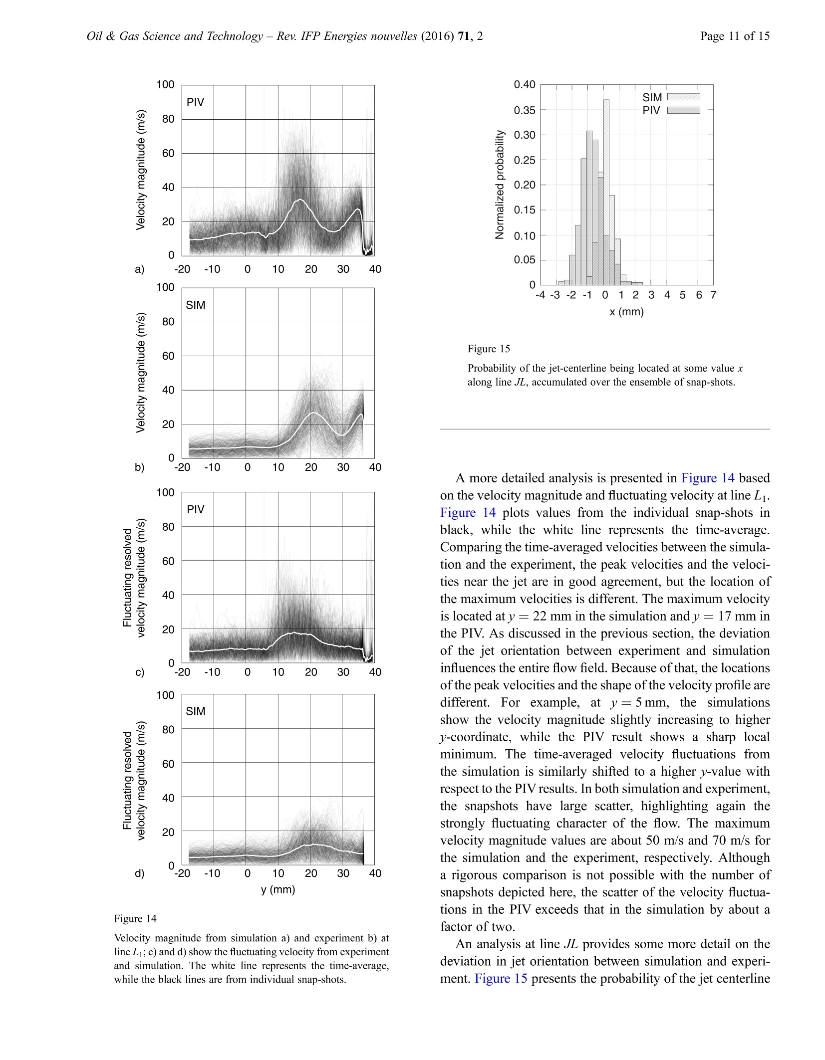
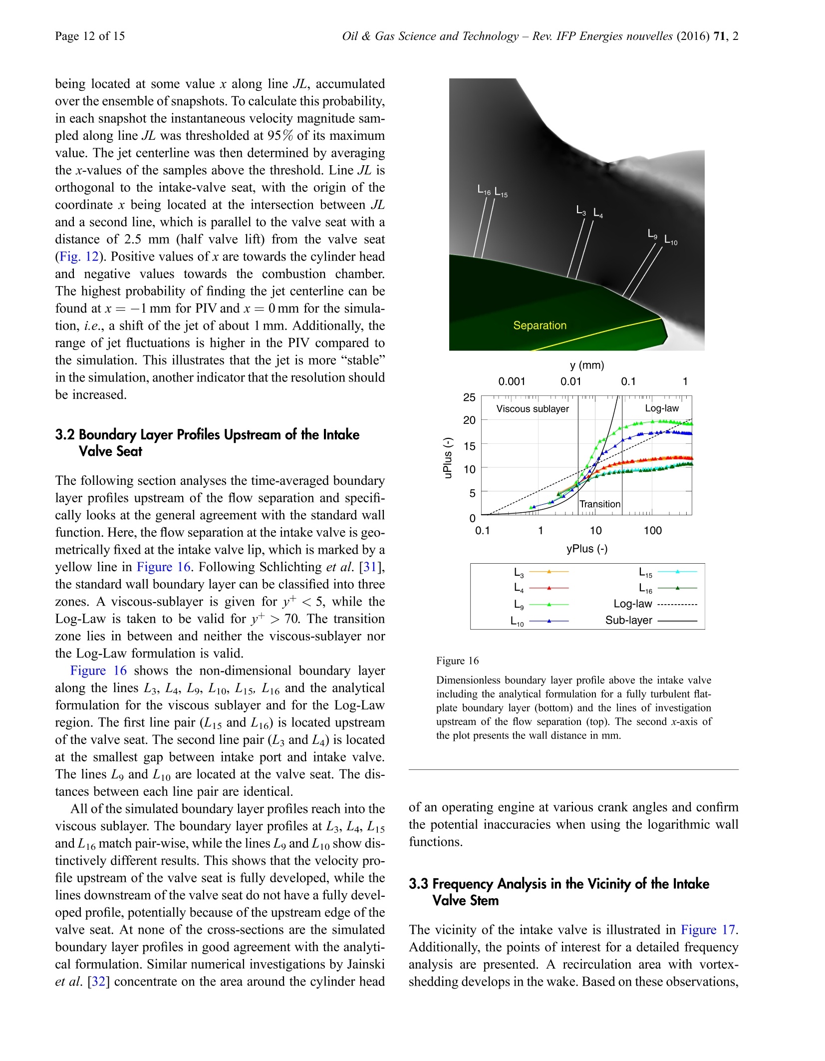
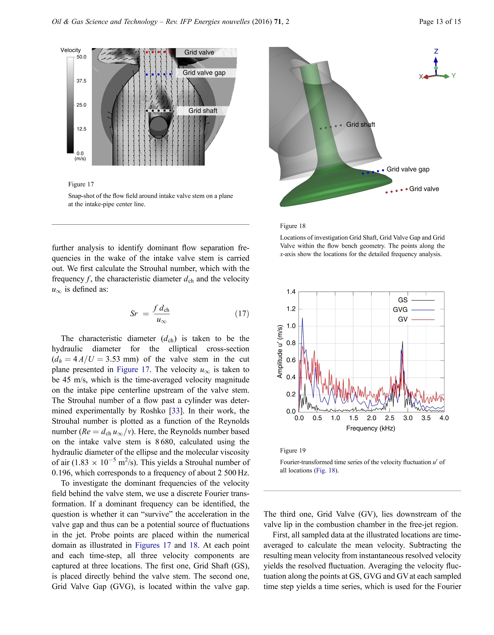
方案详情

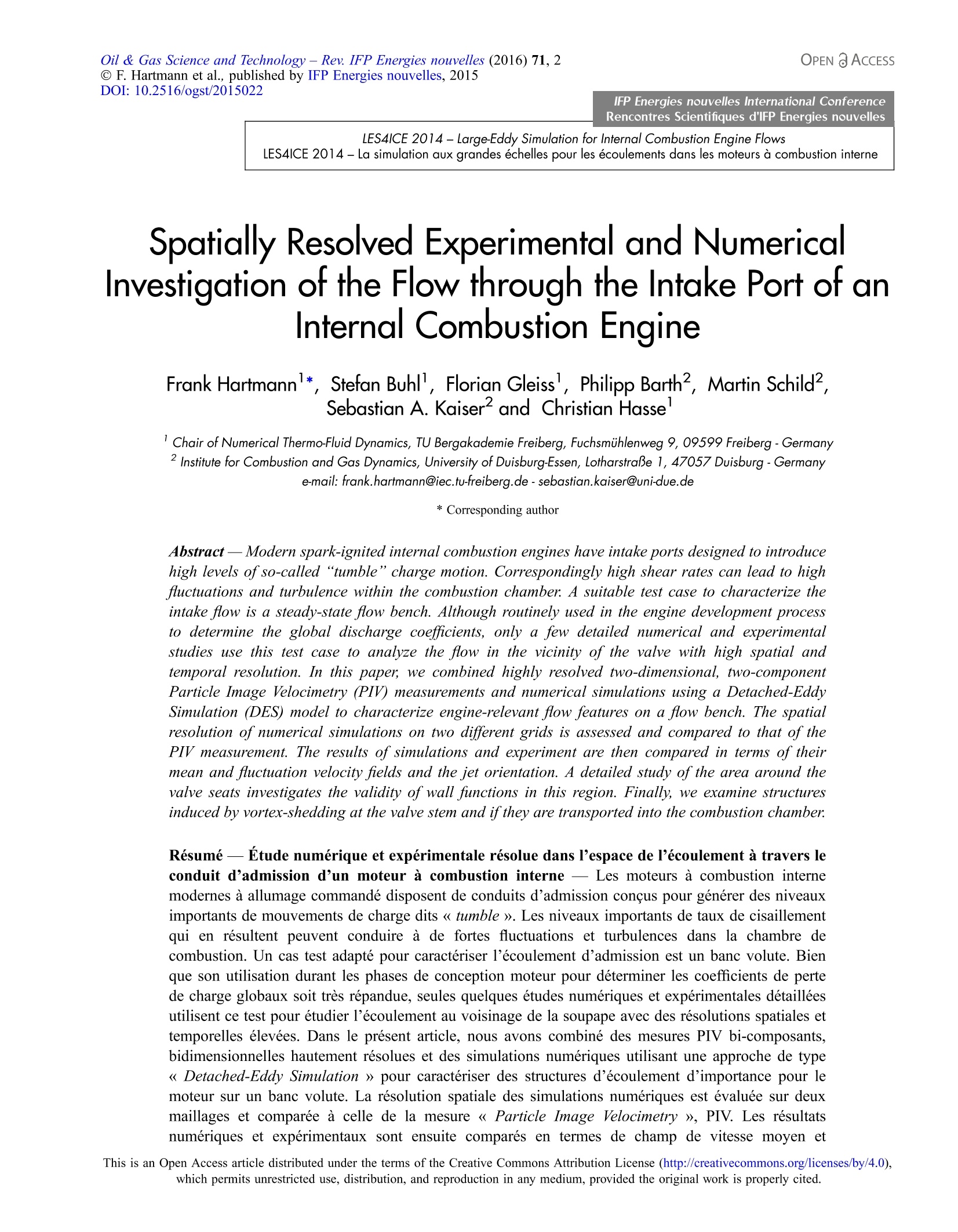
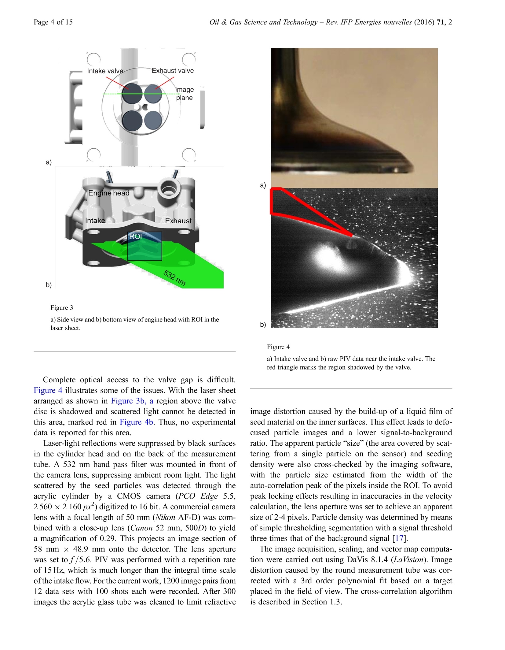
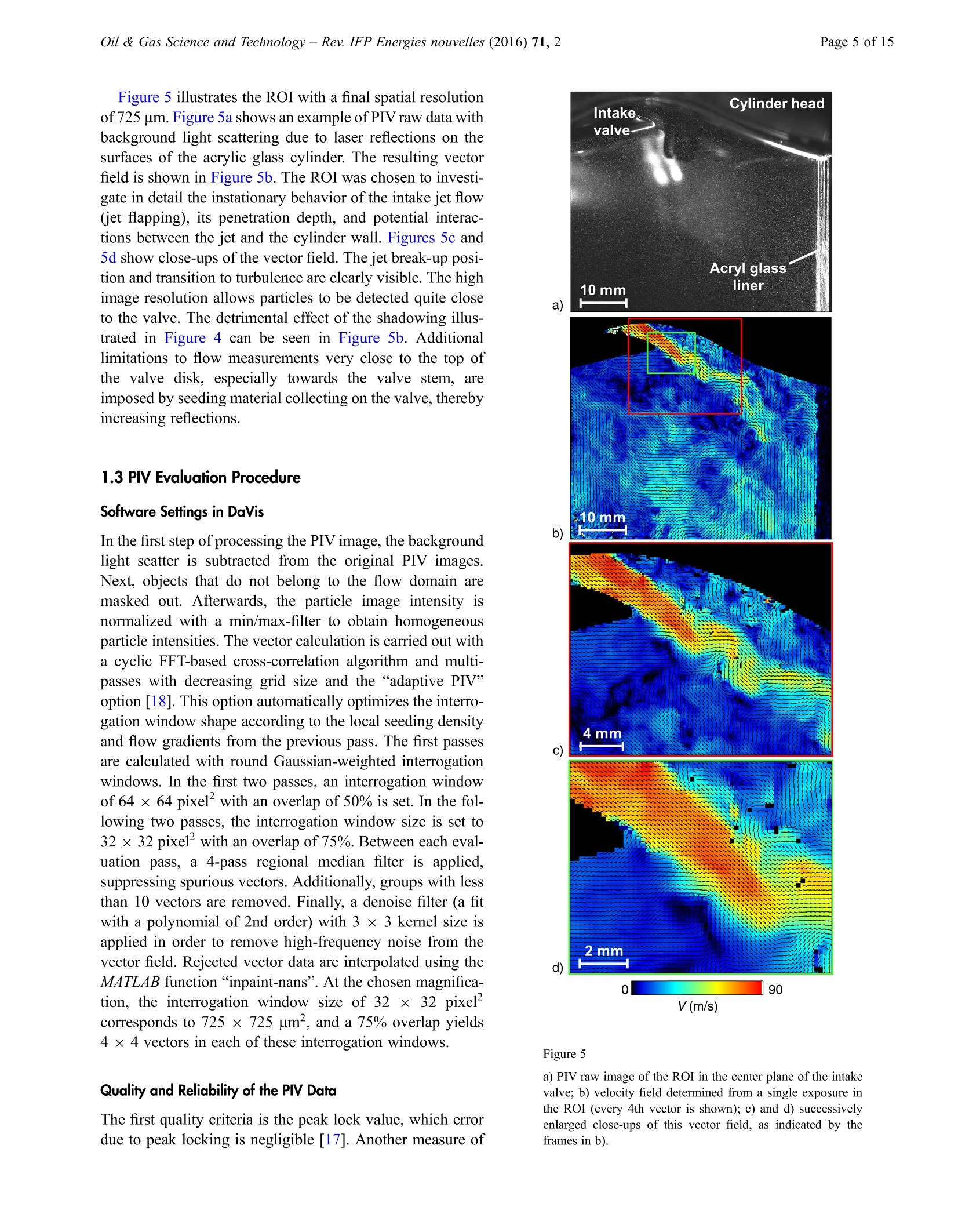
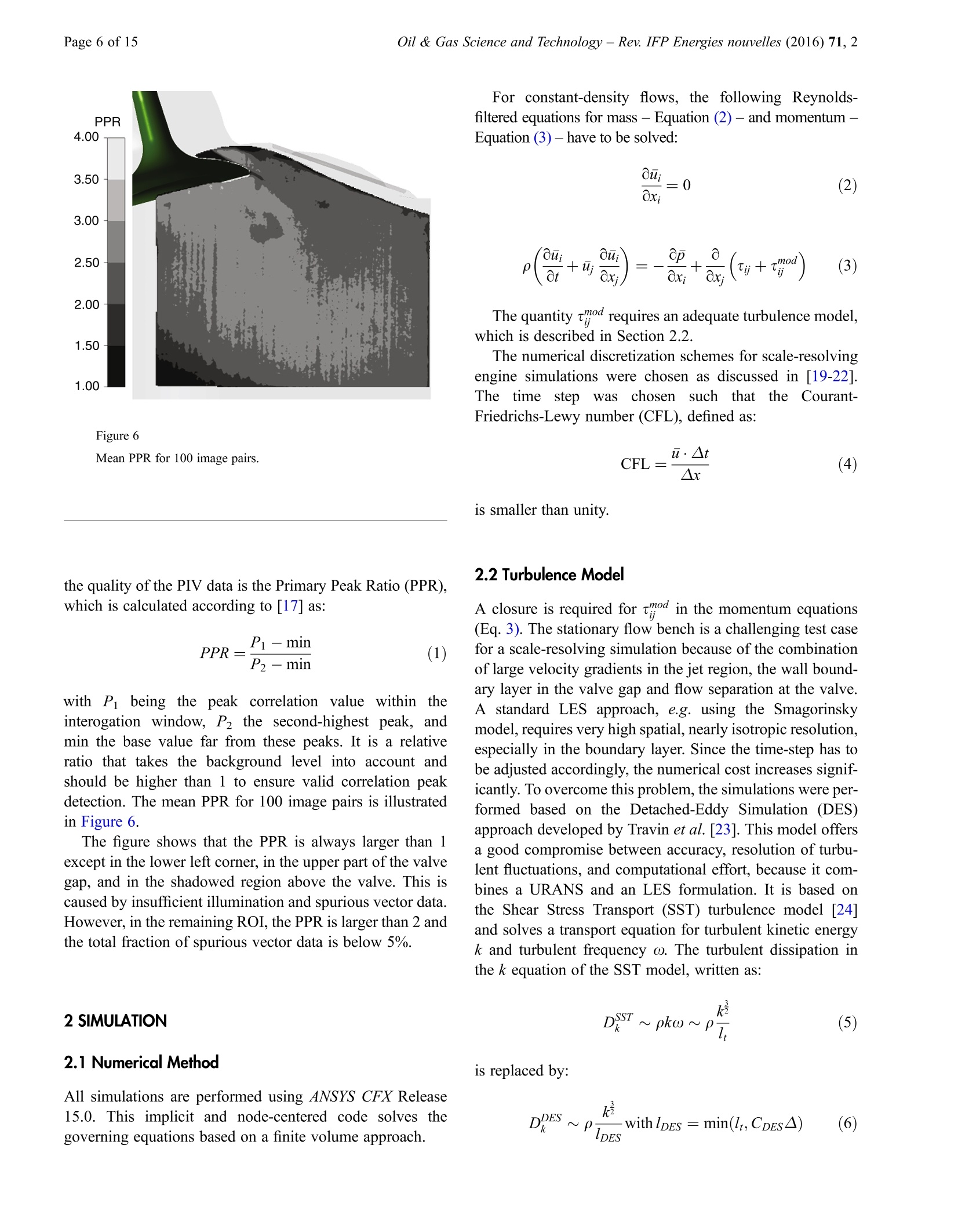
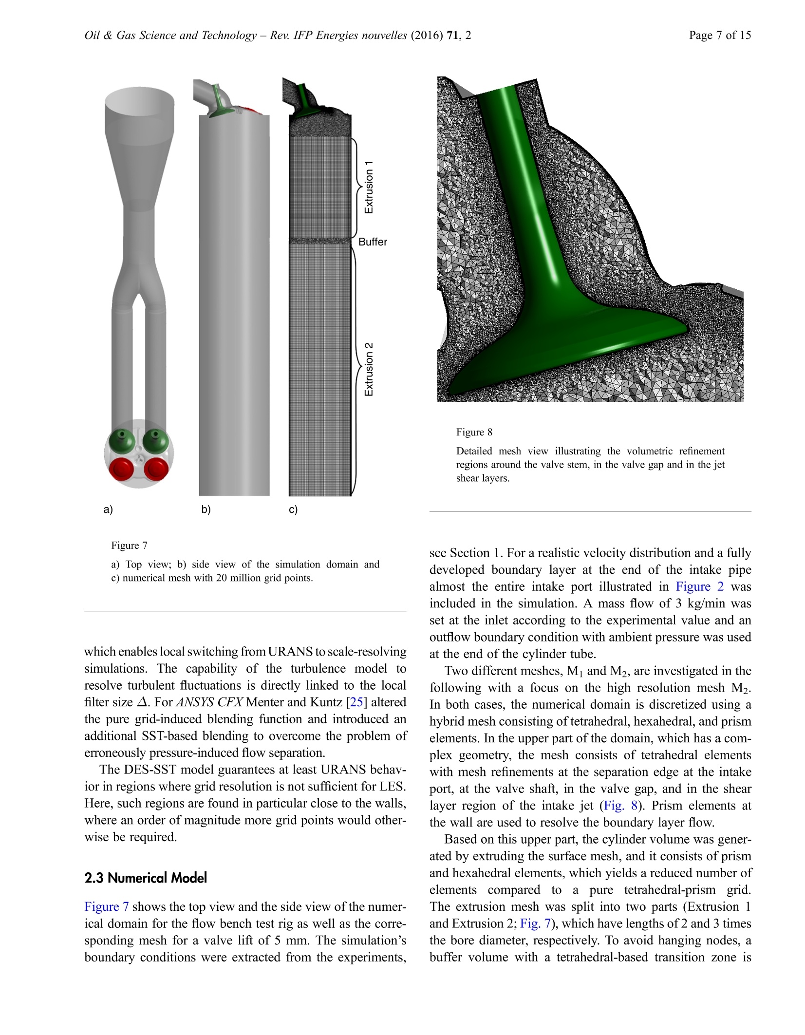
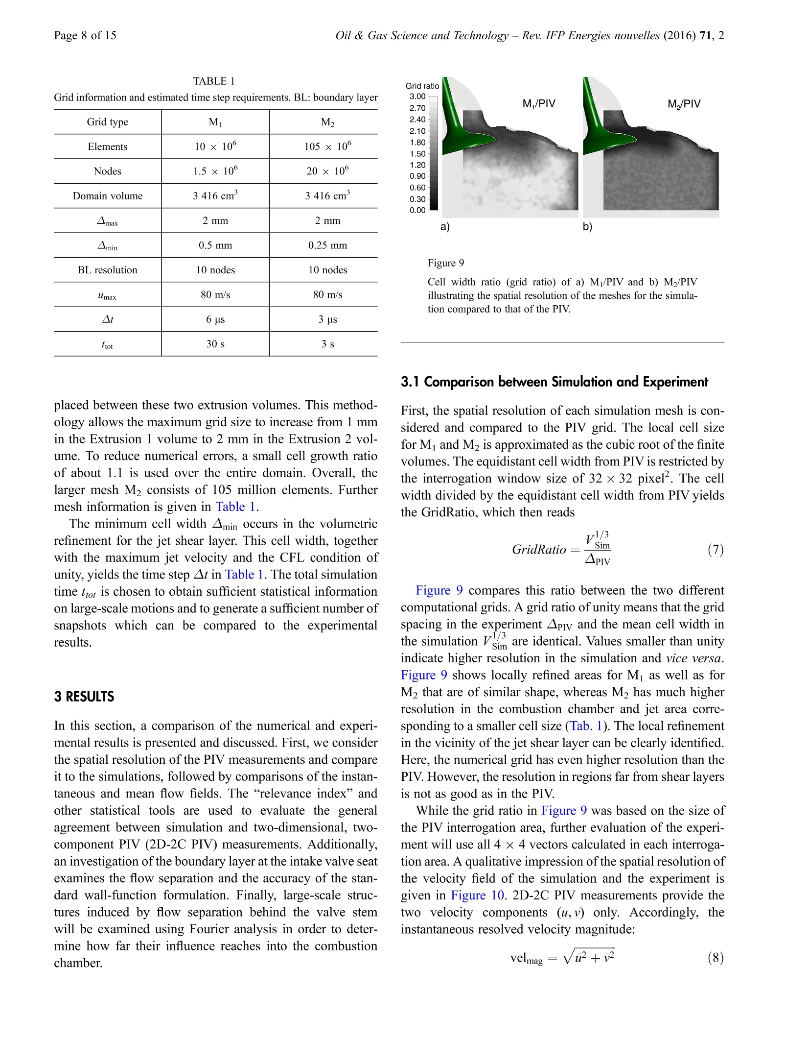
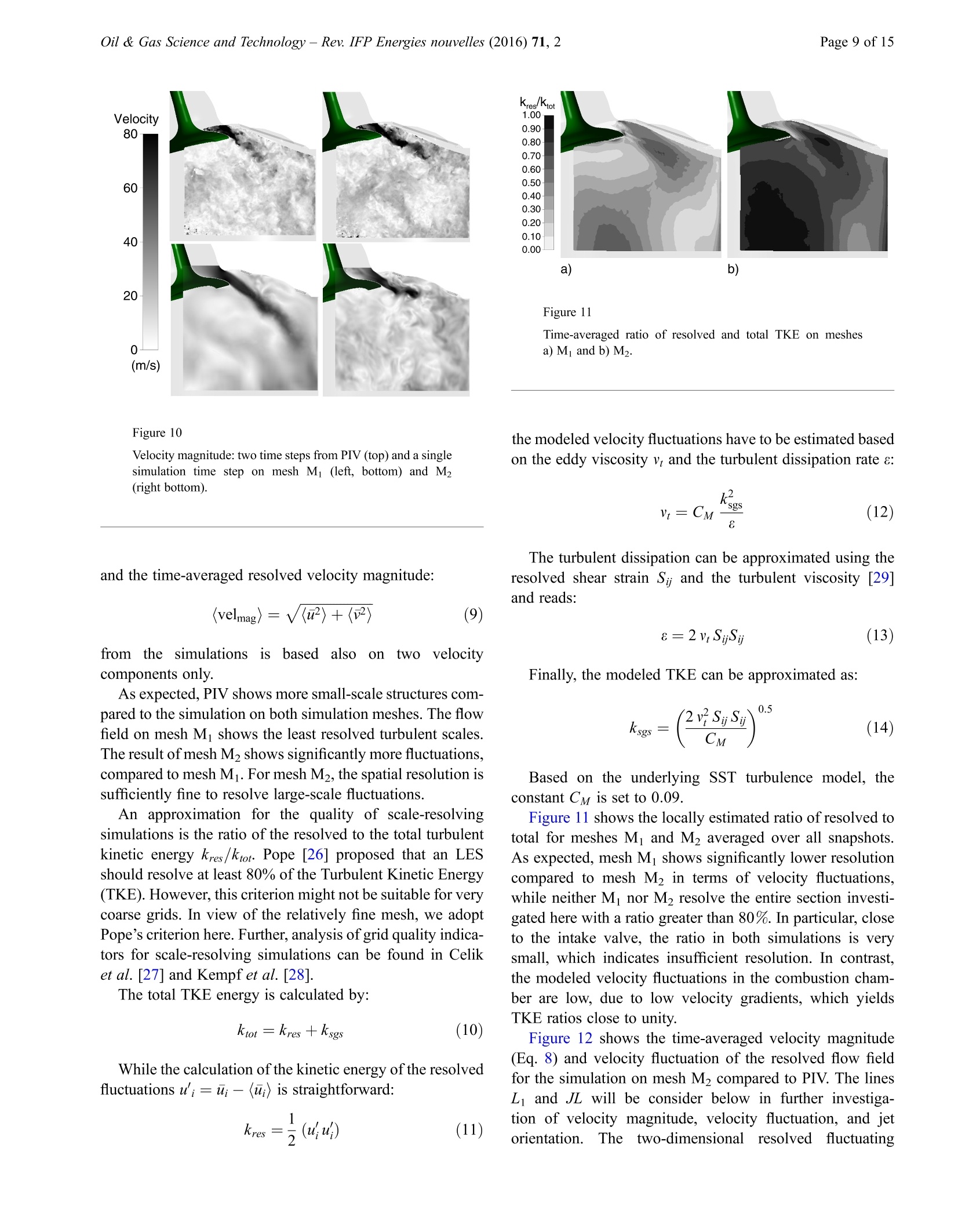
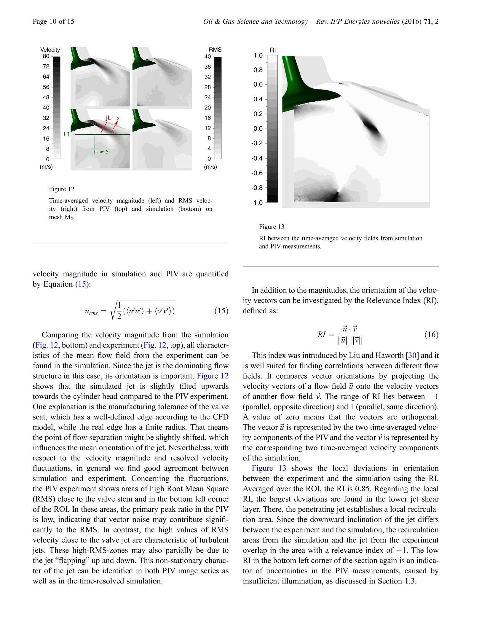
OPEN 8ACCESSOil & Gas Science and Technology - Rev. IFP Energies nouvelles (2016) 71, 2O F. Hartmann et al., published by IFP Energies nouvelles, 2015DOI: 10.2516/ogst/2015022IFP Energies nouvelles International ConferenceRencontres Scientifiques d'IFP Energies nouvellesLES4ICE 2014-Large-Eddy Simulation for Internal Combustion Engine FlowsLES4ICE 2014 - La simulation aux grandes échelles pour les écoulements dans les moteurs à combustion interne Oil & Gas Science and Technology- Rev. IFP Energies nouvelles (2016) 71, 2Page 2 of 15 Spatially Resolved Experimental and NumericalInvestigation of the Flow through the Intake Port of anInternal Combustion Engine Frank Hartmann*, Stefan Buhll, Florian Gleiss', Philipp Barth2, Martin Schild?,Sebastian A. Kaiserand Christian Hasse ' Chair of Numerical Thermo-Fluid Dynamics, TU Bergakademie Freiberg, Fuchsmuhlenweg 9, 09599 Freiberg-Germany Institute for Combustion and Gas Dynamics, University of Duisburg-Essen, LotharstraBe 1, 47057 Duisburg -Germany e-mail: frank.hartmann@iec.tu-freiberg.de-sebastian.kaiser@uni-due.de * Corresponding author Abstract - Modern spark-ignited internal combustion engines have intake ports designed to introducehigh levels of so-called “tumble”charge motion. Correspondingly high shear rates can lead to highfluctuations and turbulence within the combustion chamber. A suitable test case to characterize theintake flow is a steady-state flow bench. Although routinely used in the engine development processto determine the global discharge coefficients, only a few detailed numerical and experimentalstudies use this test case to analyze the flow in the vicinity of the valve with high spatial andtemporal resolution. In this paper, we combined highly resolved two-dimensional, two-componentParticle Image Velocimetry (PIV) measurements and numerical simulations using a Detached-EddySimulation (DES) model to characterize engine-relevant flow features on a flow bench. The spatialresolution of numerical simulations on two different grids is assessed and compared to that of thePIV measurement. The results of simulations and experiment are then compared in terms of theirmean and fuctuation velocity fields and the jet orientation. A detailed study of the area around thevalve seats investigates the validity of wall functions in this region. Finally, we examine structuresinduced by vortex-shedding at the valve stem and if they are transported into the combustion chamber Resume-Etude numerique et experimentale resolue dans Pespacede P’ecoulement a travers leconduit d'admission d'un moteur a combustion interne -Les moteurs a combustion internemodernes a allumage commande disposent de conduits d'admission concus pour generer des niveauximportants de mouvements de charge dits 《tumble》. Les niveaux importants de taux de cisaillementqui en resultent peuvent conduire a de fortes fluctuations et turbulences dans la chambre decombustion. Un cas test adapte pour caracteriser Pecoulement d'admission est un banc volute. Bienque son utilisation durant les phases de conception moteur pour determiner les coefficients de pertede charge globaux soit tres repandue, seules quelques etudes numeriques et expérimentales detailleesutilisent ce test pour etudier l’ecoulement au voisinage de la soupape avec des resolutions spatiales ettemporelles elevees. Dans le present article, nous avons combine des mesures PIV bi-composants,bidimensionnelles hautement resolues et des simulations numeriques utilisant une approche de type《Detached-Eddy Simulation 》 pour caracteriser des structures d'ecoulement d'importance pour lemoteur sur un banc volute. La resolution spatiale des simulations numeriques est evaluee sur deuxmaillages et comparee à celle de la mesure 《Particle Image Velocimetry 》, PIV. Les resultatsnumériques et expérimentaux sont ensuite compares en termes de champ de vitesse moyen et ( This i s an Open Access ar t icle d i stributed under the terms of the Creative Co m mons Attribution License (http: / / creat i vecommons.org/license s / b y/4.0), which permits u n restricted use, distribution , and reproduction in any medium, provided the original work is properly cited. ) fluctuant et d'orientation des jets. Une etude detaillee du siège de soupape est realisee pour verifier lavalidite de lois de paroi dans cette zone. Enfin, nous examinons les structures induites par lesdetachements tourbillonnaires autour de la tige de soupape et si elles sont transportees dans lachambre de combustion. The intake jet is the main contributor to the kinetic energy ofthe internal combustion engine’s in-cylinder flow. Thus, it isprimarily responsible for the development of the flow patternin the compression stroke and during combustion. Duringthe intake stroke, the intake valves throttle the incominggas flow and induce high velocities in the valve gap.Towards the combustion chamber, the resulting jet separatesfrom the valve seat and lip creating shear layers with largegradients generating turbulence [1]. During an engine cycle,the penetrating jet transports momentum through the valvegap into the combustion chamber, which initiates large-scalemotions at the beginning of the compression stroke [2]. Modern spark-ignited internal combustion engines arecharacterized by high levels of intake-induced in-cylinderflow, organized into a large-scale motion usually called“tumble". Such high levels of charge motion are achievedby flat intake ports and machined edges upstream of thevalve seat. These measures yield a non-uniform distributionof the mass flow over the intake valve, creating the distinc-tive tumble motion. In the past, there have been several investigations of theglobal in-cylinder flow and studies of the local flow-fieldnear the intake port. On the one hand, steady-state experi-ments on flow benches were performed to investigate theflow physics in a simplified configuration [3]; on the otherhand, optically accessible engines were used for measure-ments with more realistic boundary conditions [4]. A smallnumber of studies investigate the flow field in or near thevalve gap in detail. Schlieren cinematography, which isbased on density gradients, was applied to qualitativelyimage the intake jet’s motion within the cylinder of a trans-parent research engine [5]. Weclas et al. [6] used LaserDoppler Anemometry (LDA) to acquire quantitative point-wise information on the velocity and its fluctuations in thevalve gap. In a second publication, the same authors [7]discussed the flow separation in the intake valve gap insteady and transient flows under engine-like conditions.Measurements were performed using LDA and hot-wire ane-mometry. In later studies, Particle Image Velocimetry (PIV)was applied in engine geometries to measure two velocity com-ponents instantaneously, spatially resolved within a planedefined by the laser sheet [8]. In principle, with stereoscopicPIV, the out-of-plane velocity component is also accessible[9].“High-speed”PIV allows time-resolved investigations ofin-cylinderflow structures and theirdevelop-ment withinn asingle cycle,vwhilele tomographiccPIVenables volumetric measurements [10]. The mean three-dimensional flow in the intake port was fully quantifiedusingMagnetic Resonance Velocimetry((MRV) byFreudenhammer et al. [11]. On the other hand, a very limited number of numericalinvestigations of the intake flow in such flow-bench scenar-ios were performed. Mclandress et al. [12] compared PIVmeasurements and simulations on a flow bench using theKIVA-3 code. Similar studies were performed by Inagakiet al. [13] using Large-Eddy Simulations (LES) with amixed-time-scale subgrid-scale model, which were com-pared to experiments and RANS simulations. Despite the relevance of the intake flow on the chargemotion and the subsequent combustion process, no com-bined experimental-numerical studies using state-of-the-artapproaches in both areas, namely highly resolved PIV andscale-resolving flow simulations, respectively, have beenreported. This work aims to start filling this gap by applying a com-bination of PIV and LES, both at relatively high spatial res-olution, to the flow through the intake port on a flow bench.In the following section, the experiment will be describedincluding flow bench, camera, laser system and image acqui-sition. The quality and reliability of the PIV data is assessedbased on the primary peak ratio of the underlyingcross-correlation. The simulation’s general approach andgrids are discussed next. In the results, we first comparethe mean velocity fields in simulation and experiment.Further investigations on the boundary layer on the valveseat evaluate the widely-used assumption of a logarithmicwall function. Finally, large structures close to the intakevalve and the jet-flapping are examined in order to investi-gate whether such instationary structures survive the acceler-ation through the valve gap, which in an operating enginecould have an effect on the stability of the in-cylinder flow. 1 EXPERIMENT 1.1 Flow Bench The head of an optically accessible single-cylinder engine[14] is mounted on a steady-state flow bench. In previousinvestigations, this flow bench was used to determine the Figure1 Figure2 Flow diagram of the flow-bench with the two measurementpoints for pressure. cylinder head’s discharge coefficients to be used in one-dimensional engine simulations [15]. The arrangement isshown in Figure 1. A rotary blower, powered by a speed-controlled Alternating Current (AC) motor, provides thepressure difference which drives the flow. On the suctionside of the blower, a rotary piston meter measures the vol-ume flow. The temperature measured at the intake of thismeter and the atmospheric pressure are used to calculatethe mass flow. A plenum of approx. 500 L downstream ofthe piston meter eliminates flow fluctuations caused by theblower. The cylinder head is located on the pressure side of theblower. The PVC piping upstream of the head is straight,smooth-walled, and with no change in its inner diameter(d=76.6 mm) for 2 840 mm (37 d). A conical adapter con-nects the cylinder head with its intake system, which is dif-ferent in diameter, to the piping of the flow bench. Figure 2shows the geometry of the head with the components imme-diately up- and downstream. In the laboratory frame, thewhole assembly lies on its side on an optical table. Neverthe-less, throughout this paper we will refer to the orientation ofthe cylinder head, valve, and flow as if the head weremounted upright with the valves above the combustionchamber, as in a typical automotive application. In this work, a valve lift of 5 mm is fixed by a micrometerscrew pushing onto the valve cups. Only the intake port isexamined and the exhaust valves are closed. An acrylic tubewith an inner diameter of 84 mm corresponding to the boreof the engine is placed below the cylinder head as opticallyaccessible “cylinder walls". With an overall length of950 mm from the pent-roof to the outlet, it provides an CAD rendering of intake system, cylinder head, and measure-ment tube. oriented outflow into the ambient air. At two locations, thetemperature T and relative pressure p are measured: in theintake runners (reference point 1) and in the measurementtube (reference point 2, Fig. 2). Additionally, at point 1,the pressure is measured with a fast pressure transducer(Kistler 4049A5) to monitor for potential high-frequencyfluctuations in the flow. For the measurements presentedhere, only reference point 2 (and the upstream volume flowrate) is required to define the boundary conditions, butpoint 1 enables data cross-check. 1.2 Velocity Measurements In the vertical intake-valve plane, the two in-planecompo-nents of the instantaneous velocity field were measured byhigh-resolution PIV (2D-2C-PIV). Figure 3 illustrates thegeometry of the optical access on the flow bench withthe engine head, the location of the laser light sheet, andthe imaged Region Of Interest (ROI). ForrPIV. the intake air Was seeded withDi-Ethyl-Hexyl-Sebacate droplets (DEHS, nominal diameter:0.2-0.3 um). The aerosol droplets were generated by a nebu-lizer with a Laskin nozzle design [16] (LaVision, Gottingen).To ensure that the particle were homogeneously distributed,the droplets were injected through four nozzles located500 mm upstream of the intake valves. The field of viewwas illuminated by a dual-cavity, double-pulsed Nd:YAGlaser (Litron) at 532 nm with an energy of 30 mJ/pulse.Atelescopic lens arrangement formed a light sheet of0.5 mm-0.9 mm thickness, entering the ROI diagonally frombelow the head. Figure 3 a) Side view and b) bottom view of engine head with ROI in thelaser sheet. Complete optical access to the valve gap is difficult.Figure 4 illustrates some of the issues. With the laser sheetarranged as shown in Figure 3b, a region above the valvedisc is shadowed and scattered light cannot be detected inthis area, marked red in Figure 4b. Thus, no experimentaldata is reported for this area. Laser-light reflections were suppressed by black surfacesin the cylinder head and on the back of the measurementtube. A 532 nm band pass filter was mounted in front ofthe camera lens, suppressing ambient room light. The lightscattered by the seed particles was detected through theacrylic cylinder by a CMOS camera (PCO Edge 5.5,2 560 ×2160 px) digitized to 16 bit. A commercial cameralens with a focal length of 50 mm (Nikon AF-D) was com-bined with aclose-up lens (Canon 52 mm, 500D) to yielda magnification of 0.29. This projects an image section of58 mm ×48.9 mm onto the detector. The lens aperturewas set to f/5.6. PIV was performed with a repetition rateof 15 Hz, which is much longer than the integral time scaleofthe intake flow. For the current work, 1200 image pairs from12 data sets with 100 shots each were recorded. After 300images the acrylic glass tube was cleaned to limit refractive Figure 4 a) Intake valve and b) raw PIV data near the intake valve. Thered triangle marks the region shadowed by the valve. image distortion caused by the build-up of a liquid film ofseed material on the inner surfaces. This effect leads to defo-cused particle images and a lower signal-to-backgroundratio. The apparent particle“size”(the area covered by scat-tering from a single particle on the sensor) and seedingdensity were also cross-checked by the imaging software,with the particle size estimated from the width of theauto-correlation peak of the pixels inside the ROI. To avoidpeak locking effects resulting in inaccuracies in the velocitycalculation, the lens aperture was set to achieve an apparentsize of 2-4 pixels. Particle density was determined by meansof simple thresholding segmentation with a signal thresholdthree times that of the background signal [17]. The image acquisition, scaling, and vector map computa-tion were carried out using DaVis 8.1.4 (LaVision). Imagedistortion caused by the round measurement tube was cor-rected with a 3rd order polynomial fit based on a targetplaced in the field of view. The cross-correlation algorithmis described in Section 1.3. Figure 5 illustrates the ROI with a final spatial resolutionof725 pm. Figure 5a shows an example of PIV raw data withbackground light scattering due to laser reflections on thesurfaces of the acrylic glass cylinder. The resulting vectorfield is shown in Figure 5b. The ROI was chosen to investi-gate in detail the instationary behavior of the intake jet flow(jet flapping), its penetration depth, and potential interac-tions between the jet and the cylinder wall. Figures 5c and5d show close-ups of the vector field. The jet break-up posi-tion and transition to turbulence are clearly visible. The highimage resolution allows particles to be detected quite closeto the valve. The detrimental effect of the shadowing illus-trated in Figure 4 can be seen in Figure 5b. Additionallimitations to flow measurements very close to the top ofthe valve disk, especially towards the valve stem, areimposed by seeding material collecting on the valve, therebyincreasing reflections. 1.3 PIV Evaluation Procedure Software Settings in DaVis In the first step of processing the PIV image, the backgroundlight scatter is subtracted from the original PIV images.Next, objects that do not belong to the flow domain aremasked out. Afterwards, the particle image intensity isnormalized with a min/max-filter to obtain homogeneousparticle intensities. The vector calculation is carried out witha cyclic FFT-based cross-correlation algorithm and multi-passes with decreasing grid size and the “adaptive PIV”option [18]. This option automatically optimizes the interro-gation window shape according to the local seeding densityand flow gradients from the previous pass. The first passesare calculated with round Gaussian-weighted interrogationwindows. In the first two passes, an interrogation windowof 64 x 64 pixel’ with an overlap of 50% is set. In the fol-lowing two passes, the interrogation window size is set to32×32 pixel with an overlap of 75%. Between each eval-uation pass, a 4-pass regional median filter is applied,suppressing spurious vectors. Additionally, groups with lessthan 10 vectors are removed. Finally, a denoise filter (a fitwith a polynomial of 2nd order) with 3×3 kernel size isapplied in order to remove high-frequency noise from thevector field. Rejected vector data are interpolated using theMATLAB function “inpaint-nans”. At the chosen magnifica-tion, the interrogation window size of 32 × 32 pixel750corresponds to 725 ×725 um?, and a 75% overlap yields4 × 4 vectors in each of these interrogation windows. Quality and Reliability of the PIV Data The first quality criteria is the peak lock value, which errordue to peak locking is negligible [17]. Another measure of a) b) C) d) V(m/s) Figure 5 a) PIV raw image of the ROI in the center plane of the intakevalve; b)velocity field determined from a single exposure inthe ROI (every 4th vector is shown); c) and d) successivelyenlarged close-ups of this vector field, as indicated by theframes in b). Figure 6Mean PPR for 100 image pairs. the quality of the PIV data is the Primary Peak Ratio (PPR),which is calculated according to [17] as: with Pi being the peak correlation value within theinterogation window, P2 the second-highest peak, andmin the base value far from these peaks. It is a relativeratio that takes the background level into account andshould be higher than 1 to ensure valid correlation peakdetection. The mean PPR for 100 image pairs is illustratedin Figure 6. The figure shows that the PPR is always larger than 1except in the lower left corner, in the upper part of the valvegap, and in the shadowed region above the valve. This iscaused by insufficient illumination and spurious vector data.However, in the remaining ROI, the PPR is larger than 2 andthe total fraction of spurious vector data is below 5%. 2 SIMULATION 2.1 Numerical Method All simulations are performed using ANSYS CFX Release15.0. This implicit and node-centered code solves thegoverning equations based on a finite volume approach. For constant-density flows, the following Reynolds-filtered equations for mass -Equation(2)- and momentum-Equation(3)-have to be solved: The quantity od requires an adequate turbulence model,which is described in Section 2.2. The numerical discretization schemes for scale-resolvingengine simulations were chosen as discussed in [19-22].The time steppwas chosen suchtthattthe Courant-Friedrichs-Lewy number (CFL), defined as: is smaller than unity. 2.2 Turbulence Model A closure is required for rmod in the momentum equations(Eq.3). The stationary flow bench is a challenging test casefor a scale-resolving simulation because of the combinationof large velocity gradients in the jet region, the wall bound-ary layer in the valve gap and flow separation at the valve.A standard LES approach, e.g. using the Smagorinskymodel, requires very high spatial, nearly isotropic resolution,especially in the boundary layer. Since the time-step has tobe adjusted accordingly, the numerical cost increases signif-icantly. To overcome this problem, the simulations were per-formed based on the Detached-Eddy Simulation (DES)approach developed by Travin et al. [23]. This model offersa good compromise between accuracy, resolution of turbu-lent fluctuations, and computational effort, because it com-bines a URANS and an LES formulation. It is based onthe Shear Stress Transport (SST) turbulence model [24]and solves a transport equation for turbulent kinetic energyk and turbulent frequency ω. The turbulent dissipation inthe k equation of the SST model, written as: Figure 7 a) Top view; b) side view of the simulation domain andc) numerical mesh with 20 million grid points. which enables local switching fromURANS to scale-resolvingsimulations. The capability of the turbulence model toresolve turbulent fluctuations is directly linked to the localfilter size A. For ANSYS CFX Menter and Kuntz [25] alteredthe pure grid-induced blending function and introduced anadditional SST-based blending to overcome the problem oferroneously pressure-induced flow separation. The DES-SST model guarantees at least URANS behav-ior in regions where grid resolution is not sufficient for LES.Here, such regions are found in particular close to the walls,where an order of magnitude more grid points would other-wise be required. 2.3 Numerical Model Figure 7 shows the top view and the side view of the numer-ical domain for the flow bench test rig as well as the corre-sponding mesh for a valve lift of 5 mm. The simulation’sboundary conditions were extracted from the experiments, Figure 8 Detailed mesh view illustrating the volumetric refinementregions around the valve stem, in the valve gap and in the jetshear layers. see Section 1. For a realistic velocity distribution and a fullydeveloped boundary layer at the end of the intake pipealmost the entire intake port illustrated in Figure 2 wasincluded in the simulation. A mass flow of 3 kg/min wasset at the inlet according to the experimental value and anoutflow boundary condition with ambient pressure was usedat the end of the cylinder tube. Two different meshes, M and M2, are investigated in thefollowing with a focus on the high resolution mesh M.In both cases, the numerical domain is discretized using ahybrid mesh consisting of tetrahedral, hexahedral, and prismelements. In the upper part of the domain, which has a com-plex geometry, the mesh consists of tetrahedral elementswith mesh refinements at the separation edge at the intakeport, at the valve shaft, in the valve gap, and in the shearlayer region of the intake jet (Fig. 8). Prism elements atthe wall are used to resolve the boundary layer flow. Based on this upper part, the cylinder volume was gener-ated by extruding the surface mesh, and it consists of prismand hexahedral elements, which yields a reduced number ofelementss(compared to aapure tetrahedral-prism grid.The extrusion mesh was split into two parts (Extrusion ]and Extrusion 2; Fig. 7), which have lengths of 2 and 3 timesthe bore diameter, respectively. To avoid hanging nodes, abuffer volume with a tetrahedral-based transition zone is TABLE lGrid information and estimated time step requirements. BL: boundary layer Grid type M M2 Elements 10 × 10° 105×10° Nodes 1.5×10° 20×10° Domain volume 3 416 cm 3 416 cm' Amax 2 mm 2 mm Amin 0.5 mm 0.25 mm BL resolution 10 nodes 10 nodes Umax 80 m/s 80 m/s At 6 us 3 us ttot 30 s 3 s placed between these two extrusion volumes. This method-ology allows the maximum grid size to increase from 1 mmin the Extrusion 1 volume to 2 mm in the Extrusion 2 vol-ume. To reduce numerical errors, a small cell growth ratioof about 1.1 is used over the entire domain. Overall, thelarger mesh M2 consists of 105 million elements. Furthermesh information is given in Table 1. The minimum cell width Amin occurs in the volumetricrefinement for the jet shear layer. This cell width, togetherwith the maximum jet velocity and the CFL condition ofunity, yields the time step At in Table 1. The total simulationtime ttot is chosen to obtain sufficient statistical informationon large-scale motions and to generate a sufficient number ofsnapshots which can be compared to the experimentalresults. 3 RESULTS In this section, a comparison of the numerical and experi-mental results is presented and discussed. First, we considerthe spatial resolution of the PIV measurements and compareit to the simulations, followed by comparisons of the instan-taneous and mean flow fields. The “relevance index” andother statistical tools are used to evaluate the generalagreement between simulation and two-dimensional, two-component PIV (2D-2C PIV) measurements. Additionally,an investigation of the boundary layer at the intake valve seatexamines the flow separation and the accuracy of the stan-dard wall-function formulation. Finally, large-scale struc-tures induced by flow separation behind the valve stemwill be examined using Fourier analysis in order to deter-mine how far their influence reaches into the combustionchamber. Figure 9 Cell width ratio (grid ratio) of a) M/PIV and b) M2/PIVillustrating the spatial resolution of the meshes for the simula-tion compared to that of the PIV. 3.1 Comparison between Simulation and Experiment First, the spatial resolution of each simulation mesh is con-sidered and compared to the PIV grid. The local cell sizefor M and M2 is approximated as the cubic root of the finitevolumes. The equidistant cell width from PIV is restricted bythe interrogation window size of 32 ×32 pixel. The cellwidth divided by the equidistant cell width from PIV yieldsthe GridRatio, which then reads Figure 9 compares this ratio between the two differentcomputational grids. A grid ratio ofunity means that the gridspacing in the experiment Aply and the mean cell width inthe simulation Vare identical. Values smaller than unityindicate higher resolution in the simulation and vice versa.Figure 9 shows locally refined areas for M as well as forM2 that are of similar shape, whereas Mz has much higherresolution in the combustion chamber and jet area corre-sponding to a smaller cell size (Tab.1). The local refinementin the vicinity of the jet shear layer can be clearly identified.Here, the numerical grid has even higher resolution than thePIV. However, the resolution in regions far from shear layersis not as good as in the PIV. While the grid ratio in Figure 9 was based on the size ofthe PIV interrogation area, further evaluation of the experi-ment will use all 4 x4 vectors calculated in each interroga-tion area. A qualitative impression of the spatial resolution ofthe velocity field of the simulation and the experiment isgiven in Figure 10. 2D-2C PIV measurements provide thetwo velocity components (u,v) only. Accordingly, theinstantaneous resolved velocity magnitude: Figure 10 Velocity magnitude: two time steps from PIV (top) and a singlesimulation time step on mesh M (left, bottom) and M2(right bottom). and the time-averaged resolved velocity magnitude: from the simulations is based also ontwo velocitycomponents only. As expected, PIV shows more small-scale structures com-pared to the simulation on both simulation meshes. The flowfield on mesh M shows the least resolved turbulent scales.The result of mesh Mzshows significantly more fluctuations,compared to mesh M. For mesh M2, the spatial resolution issufficiently fine to resolve large-scale fluctuations. An approximation for the quality of scale-resolvingsimulations is the ratio of the resolved to the total turbulentkinetic energy kres/ktot. Pope [26] proposed that an LESshould resolve at least 80% of the Turbulent Kinetic Energy(TKE). However, this criterion might not be suitable for verycoarse grids. In view of the relatively fine mesh, we adoptPope’s criterion here. Further, analysis of grid quality indica-tors for scale-resolving simulations can be found in Celiket al.[27] and Kempf et al.[28]. The total TKE energy is calculated by: While the calculation of the kinetic energy of the resolvedfluctuations u'i =u;一(ui) is straightforward: Figure 11 Time-averaged ratio of resolved and total TKE on meshesa) Mi and b) M2 the modeled velocity fluctuations have to be estimated basedon the eddy viscosity vr and the turbulent dissipation rate : The turbulent dissipation can be approximated using theresolved shear strain Sy and the turbulent viscosity [29]and reads: Finally, the modeled TKE can be approximated as: Based on the underlying SST turbulence model, theconstant CM is set to 0.09. Figure 11 shows the locally estimated ratio of resolved tototal for meshes M and M2 averaged over all snapshots.As expected, mesh M shows significantly lower resolutioncompared to mesh M2 in terms of velocity fluctuations,while neither M nor M2 resolve the entire section investi-gated here with a ratio greater than 80%. In particular, closeto the intake valve, the ratio in both simulations is verysmall, which indicates insufficient resolution. In contrast,the modeled velocity fluctuations in the combustion cham-ber are low, due to low velocity gradients, which yieldsTKE ratios close to unity. Figure 12 Time-averaged velocity magnitude (left) and RMS veloc-ity (right) from PIVV((top) and simulation (bottom)) onmesh M. velocity magnitude in simulation and PIV are quantifiedby Equation (15): Comparing the velocity magnitude from the simulation(Fig. 12,bottom) and experiment (Fig. 12, top), all character-istics of the mean flow field from the experiment can befound in the simulation. Since the jet is the dominating flowstructure in this case, its orientation is important. Figure 12shows that the simulated jet is slightly tilted upwardstowards the cylinder head compared to the PIV experiment.One explanation is the manufacturing tolerance of the valveseat, which has a well-defined edge according to the CFDmodel, while the real edge has a finite radius. That meansthe point of flow separation might be slightly shifted, whichinfluences the mean orientation of the jet. Nevertheless, withrespect to the velocity magnitude and resolved velocityfluctuations, in general we find good agreement betweensimulation and experiment. Concerning the fluctuations,the PIV experiment shows areas of high Root Mean Square(RMS) close to the valve stem and in the bottom left cornerof the ROI. In these areas, the primary peak ratio in the PIVis low, indicating that vector noise may contribute signifi-cantly to the RMS. In contrast, the high values of RMSvelocity close to the valve jet are characteristic of turbulentjets. These high-RMS-zones may also partially be due tothe jet “flapping”up and down. This non-stationary charac-ter of the jet can be identified in both PIV image series aswell as in the time-resolved simulation. Figure 13 RI between the time-averaged velocity fields from simulationand PIV measurements. In addition to the magnitudes, the orientation of the veloc-ity vectors can be investigated by the Relevance Index (RI),defined as: This index was introduced by Liu and Haworth [30] and itis well suited for finding correlations between different flowfields. It compares vector orientations by projecting thevelocity vectors of a flow field u onto the velocity vectorsof another flow field v. The range of RI lies between -1(parallel, opposite direction) and 1 (parallel, same direction).A value of zero means that the vectors are orthogonal.The vector u is represented by the two time-averaged veloc-ity components of the PIV and the vector V is represented bythe corresponding two time-averaged velocity componentsof the simulation. Figure 13 shows the local deviations in orientationbetween the experiment and the simulation using the RI.Averaged over the ROI, the RI is 0.85. Regarding the localRI, the largest deviations are found in the lower jet shearlayer. There, the penetrating jet establishes a local recircula-tion area. Since the downward inclination of the jet differsbetween the experiment and the simulation, the recirculationareas from the simulation and the jet from the experimentoverlap in the area with a relevance index of -1. The lowRI in the bottom left corner of the section again is an indica-tor of uncertainties in the PIV measurements, caused byinsufficient illumination, as discussed in Section 1.3. 100 SIM 80E0co> 60 40 20 d) -20 -10 O 10 20 30 40 y (mm) Figure 14 Velocity magnitude from simulation a) and experiment b) atlineLi; c) and d) show the fluctuating velocity from experimentand simulation. The white line represents the time-average,while the black lines are from individual snap-shots. Figure 15 Probability of the jet-centerline being located at some value xalong line JL, accumulated over the ensemble of snap-shots. A more detailed analysis is presented in Figure 14 basedon the velocity magnitude and fluctuating velocity at line Lj.Figure 14 plots values from the individual snap-shots inblack, while the white line represents the time-average.Comparing the time-averaged velocities between the simula-tion and the experiment, the peak velocities and the veloci-ties near the jet are in good agreement, but the location ofthe maximum velocities is different. The maximum velocityis located at y=22 mm in the simulation and y= 17 mm inthe PIV. As discussed in the previous section, the deviationof the jet orientation between experiment and simulationinfluences the entire flow field. Because of that, the locationsof the peak velocities and the shape of the velocity profile aredifferent. For example, at y=5mm, the simulationsshow the velocity magnitude slightly increasing to highery-coordinate, while the PIV result shows a sharp localminimum. The time-averaged velocity fluctuations fromthe simulation is similarly shifted to a higher y-value withrespect to the PIV results. In both simulation and experiment,the snapshots have large scatter, highlighting again thestrongly fluctuating character of the flow. The maximumvelocity magnitude values are about 50 m/s and 70 m/s forthe simulation and the experiment, respectively. Althougha rigorous comparison is not possible with the number ofsnapshots depicted here, the scatter of the velocity fluctua-tions in the PIV exceeds that in the simulation by about afactor of two. An analysis at line JL provides some more detail on thedeviation in jet orientation between simulation and experi-ment. Figure 15 presents the probability of the jet centerline being located at some value x along line JL, accumulatedover the ensemble of snapshots. To calculate this probability,in each snapshot the instantaneous velocity magnitude sam-pled along line JL was thresholded at 95% of its maximumvalue. The jet centerline was then determined by averagingthe x-values of the samples above the threshold. Line JL isorthogonal to the intake-valve seat, with the origin of thecoordinate x being located at the intersection between JLand a second line, which is parallel to the valve seat with adistance of 2.5 mm (half valve lift) from the valve seat(Fig.12). Positive values of x are towards the cylinder headand negative values towards the combustion chamber.The highest probability of finding the jet centerline can befound at x= -1mm for PIV and x = 0mm for the simula-tion, i.e., a shift of the jet of about 1 mm. Additionally, therange of jet fluctuations is higher in the PIV compared tothe simulation. This illustrates that the jet is more“stable”in the simulation,another indicator that the resolution shouldbe increased. 3.2 Boundary Layer Profiles Upstream of the IntakeValve Seat The following section analyses the time-averaged boundarylayer profiles upstream of the flow separation and specifi-cally looks at the general agreement with the standard wallfunction. Here, the flow separation at the intake valve is geo-metrically fixed at the intake valve lip, which is marked by ayellow line in Figure16. Following Schlichting et al. [31],the standard wall boundary layer can be classified into threezones. A viscous-sublayer is given for y<5, while theLog-Law is taken to be valid for y> 70. The transitionzone lies in between and neither the viscous-sublayer northe Log-Law formulation is valid. Figure 16 shows the non-dimensional boundary layeralong the lines L3, L4, L9, L10, L15, L16 and the analyticalformulation for the viscous sublayer and for the Log-Lawregion. The first line pair (Li5 and L16) is located upstreamofthe valve seat. The second line pair (L3 and L4) is locatedat the smallest gap between intake port and intake valve.The lines Lg and L1o are located at the valve seat. The dis-tances between each line pair are identical. All of the simulated boundary layer profiles reach into theviscous sublayer. The boundary layer profiles at L3, L4, Lisand L16 match pair-wise, while the lines Lg and L1o show dis-tinctively different results. This shows that the velocity pro-file upstream of the valve seat is fully developed, while thelines downstream of the valve seat do not have a fully devel-oped profile, potentially because of the upstream edge of thevalve seat. At none of the cross-sections are the simulatedboundary layer profiles in good agreement with the analyti-cal formulation. Similar numerical investigations by Jainskiet al. [32] concentrate on the area around the cylinder head Sub-layer - Figure 16 Dimensionless boundary layer profile above the intake valveincluding the analytical formulation for a fully turbulent flat-plate boundary layer (bottom) and the lines of investigationupstream of the flow separation (top). The second x-axis ofthe plot presents the wall distance in mm. of an operating engine at various crank angles and confirmthe potential inaccuracies when using the logarithmic wallfunctions. 3.3 Frequency Analysis in the Vicinity of the IntakeValve Stem The vicinity of the intake valve is illustrated in Figure 17.Additionally, the points of interest for a detailed frequencyanalysis are presented. A recirculation area with vortex-shedding develops in the wake. Based on these observations, Figure 17 Snap-shot of the flow field around intake valve stem on a planeat the intake-pipe center line. further analysis to identify dominant flow separation fre-quencies in the wake of the intake valve stem is carriedout. We first calculate the Strouhal number, which with thefrequency f, the characteristic diameter dch and the velocityu is defined as: The characteristic diameter (dch) is taken to be thehydraulicdiameter forrtheeellipticalcross-section(dh=4A/U=3.53 mm) of the valve stem in the cutplane presented in Figure 17. The velocity uo is taken tobe 45 m/s, which is the time-averaged velocity magnitudeon the intake pipe centerline upstream of the valve stem.The Strouhal number of a flow past a cylinder was deter-mined experimentally by Roshko [33]. In their work, theStrouhal number is plotted as a function of the Reynoldsnumber (Re=dchUc/v). Here, the Reynolds number basedon the intake valve stem is 8680, calculated using thehydraulic diameter of the ellipse and the molecular viscosityof air (1.83×10-m²/s). This yields a Strouhal number of0.196, which corresponds to a frequency of about 2 500 Hz. To investigate the dominant frequencies of the velocityfield behind the valve stem, we use a discrete Fourier trans-formation. If a dominant frequency can be identified, thequestion is whether it can“survive"the acceleration in thevalve gap and thus can be a potential source of fluctuationsin the jet. Probe points are placed within the numericaldomain as illustrated in Figures 17 and 18. At each pointand each time-step, all three velocity components arecaptured at three locations. The first one, Grid Shaft (GS),is placed directly behind the valve stem. The second one,Grid Valve Gap (GVG), is located within the valve gap. Y Figure 18 Locations of investigation Grid Shaft, Grid Valve Gap and GridValve within the flow bench geometry. The points along thex-axis show the locations for the detailed frequency analysis. Figure 19 Fourier-transformed time series of the velocity fluctuation u’ ofall locations (Fig. 18). The third one, Grid Valve (GV), lies downstream of thevalve lip in the combustion chamber in the free-jet region. First, all sampled data at the illustrated locations are time-averaged to calculate the mean velocity. Subtracting theresulting mean velocity from instantaneous resolved velocityyields the resolved fluctuation. Averaging the velocity fluc-tuation along the points at GS, GVG and GV at each sampledtime step yields a time series, which is used for the Fourier analysis. The Fourier analysis of each velocity componentshows that indeed there is a dominant frequency in the fluc-tuating velocity component u'in x-direction. The amplitudesof the velocity fluctuations u are presented in Figure 19. The location GS shows a significant fluctuation peak at2 860 Hz, which corresponds approximately to that calculatedfrom the Strouhal number. The locations GVG and GV show abroader range of relevant frequencies, but a distinctive peak at2860 Hz can still be detected. The importance ofother frequen-cies increase with increasing distance from the valve stem.Overall, the analysis indicates that the vortex structure behindthe valve stem survives the acceleration through the valve gapinto the combustion chamber SUMMARY This work investigated the unsteady flow through the intakevalve of a typical spark-ignited engine’s cylinder head andhow it influences the jet entering the combustion chamber.With the cylinder head on a flow bench, the valve lift wasfixed at 5 mm. The study utilized two-dimensional, two-component highly-resolved PIV and scale-resolving simula-tions on two different grids. Instantaneous flow fieldsillustrate the high resolution of the experimental data andlocally even finer structures could be resolved than in thesimulations on the finest grid. Generally, good agreementbetween the numerical and experimental velocity fieldswas observed. Statistical analysis of field-wide quantitiesas well as more detailed examination along selected line cutsthrough the data reveal some differences between experi-ment and simulation, in particular, in the orientation of theintake jet. Based on this, we suggest that even higher resolu-tions for the CFD simulation close to the jet should be thescope of future studies. An analysis of the boundary layer profiles above the valvein the vicinity of the separation point revealed that the com-monly-used wall formulation for y+> 70 was not applicableand the simulation grid should be fine enough to place thefirst grid point in the viscous sublayer as it is done here. Finally, we investigated the vortex shedding at the valvestem. A Fourier analysis to identify dominant frequenciesand a Strouhal-number-based approximation were com-pared. The Fourier analysis identified a dominant frequencyat 2 860 Hz in the wake of the stem, which is close to theStrouhal approximation of 2 500 Hz. This frequency wasalso found in the fluctuating velocity in the combustionchamber, downstream of the acceleration between the valveand its seat. This indicates that such vortices generatedupstream of the valve gap can influence the flow field asfar downstream as the combustion chamber and thus in anoperating engine could be a potential trigger of cyclicvariations. ACKNOWLEDGMENTS The authors kindly acknowledge the financial support by theSaxon Ministry of Science and Fine Arts, the SAB and theEuropean Union in the project ,,DynMo” (project number100113147), the Forschungsvereinigung Verbrennungsmot-oren (FVV) and the Deutsche Forschungsgemeinschaft(DFG) in the project “BSZ II” (FVV project number6011333, DFG project ID Schu 1369/11-2)) andl theRiickkehrerprogramm of the NRW Ministry for Innovation,Science, and Research. The simulations were performed onthe national supercomputer Cray XC40 (Hornet) at the HighPerformance Computing Center Stuttgart (HLRS) under thegrant number ICECCV/44054. REFERENCES ( 1 B icen A .F., V afidis C., Whitelaw J.H. (1985) Steady and unsteady a irflow through t h e in t ake va l ve of rec i procatingengine, Journal of Fluids E n gineering, Tr a nsactions of the ASME 107, 3, 413-420. ) ( 2 H eywood J.B. (1988) Internal combustion engine fundamen- tals , Mcgraw-Hill, New York. ) ( 3 I mberdis O ., Hartmann M ., B ensler H., Kapitza L., TheveninD. (2007) A n umerical a nd e x perimental i n vestigation of a DISI-engine intake port gegneenreartaetde d t i turbulen t flow. SAE Technical Paper 2007-01-4047. ) ( 4 S tansfield P., Wigley G . , Justham T. , Catto J., Pitcher G. (2007)PIV analysis of i n-cylinder flow structures over a r ange of r ealisti c engine speeds, ExperimentsS 1 in F luids 43, 1,135-146. ) ( 5 N amazian M . , H a nsen S., L y ford-Pike E . , S anchez-Barsse J., Heywood J., Rife J. (1980) Sc h lieren visualization of the flow and d ensity fields i n t he c ylinder of a spark-ignition engine,SAE Technical Paper 800044. ) ( 6 W eclas M., Melling A., Durst F. (1995) Unsteady intake valve gap flows, SAE Technical Paper 952477. ) ( 7 W V eclas M., Melling A.,Durst F.(1998) Flow separation in th e inlet valve gap of p iston engines, Progress i n E nergy a n d Combustion Science 24, 3 , 1 65-195. ) 8VValentino G., Kaufman D., Farrell P. (1993) Intake valve flowmeasurements using PIV, SAE Technical Paper 932700. 9 Bicker I., Karhoff D.C., Klaas M., Schroder W. (2012) Stereo-scopic multi-planar PIV measurements of in-cylinder tumblingflow, Experiments in Fluids 53, 6, 1993-2009. ( 10 B aum E., P e terson B . , Surmann C. , Mi c haelis D. , Bo h m B.,Dreizler A. ( 2013) I n vestigation of the 3D flo w field in a n IC engine using tomographic PIV, Proceedings of the CombustionInstitute 34,2,2903-2910. ) 11 Freudenhammer D., Baum E., Peterson B., Bohm B., Jung B.,Grundmann S. (2014) Volumetric intake flow measurements ofan IC engine using magnetic resonance velocimetry, Experi-ments in Fluids 55, 5. 12 McLandress A., Emerson R.,McDowell P.,Rutland C. (1996)Intake and in-cylinder flow modeling characterization of mix-ing and comparison with flow bench results, SAE TechnicalPaper 960635. 13 Inagaki M., Nagaoka M., Horinouchi N., Suga K. (2010) Largeeddy simulation analysis of engine steady intake flows using amixed-time-scale subgrid-scale model, International Journal ofEngine Research 11, 3, 229-241. 14 Kaiser S.A.,Schild M., Schulz C. (2013) Thermal stratificationin an internal combustion engine due to wall heat transfermeasured by laser-induced fluorescence, Proceedings of theCombustion Institute 34, 2, 2911-2919. ( 15 Gessenhardt C . (2013) Endoskopische Bestimmung des Temperaturfeldes im Brennraum v on O t tomotoren mittels laserinduzierter r F Fluoreszenz. PhD Thesis. Universitat Duisburg-Essen. ) 16 Melling A. (1997) Tracer particles and seeding for particleimage velocimetry, Measurement Science and Technology 8,12,1406-416. 17 LaVision (2013) Product-Manual Flow Master for DaVis 8.1. 18 Wieneke B., Pfeiffer K. (2010) Adaptive PIV with variable inter-rogation window size and shape, 15th International Symposiumon Applications of Laser Techniques to Fluid Mechanics. ( 19 H asse C., Sohm V., D urst B. (2009) Detached e ddy simulation of cyclic l arge s cale f luctuations in a simplified engine setup,International Journal ofHeat and F l uid Flow 30, 1, 32 -43. ) 20 Hasse C., Sohm V., Wetzel M., Durst B. (2009) HybridURANS/LES turbulence simulation of vortex shedding behinda triangular flameholder, Flow, Turbulence and Combustion 83,1, 1-20. 21 Hasse C., Sohm V., Durst B. (2010) Numerical investigation ofcyclic variations in gasoline engines using a hybrid URANS/LES modeling approach, Computers and Fluids 39,1, 25-48. 22 SohmV. (2007) Hybrid turbulence simulation to predict cyclicvariations in internal combustion engines, PhD Thesis, RWTHAachen. 23 TTravin A., Shur M., Strelets M., Spalart P.R. (2004) Physicaland numerical upgrades in the detached-eddy simulation ofcomplex turbulent flows, Fluid Mechanics and its Applications65, 239-254. 24 Menter F.R. (1994) Two-equation eddy-viscosity turbulencemodels for engineering applications, AIAA journal 32, 8,1598-1605. 25 Menter F.R., Kuntz M. (2003) Development and application ofa zonal DES turbulence model for CFX-5, ANYSYS CFX val-idation report, Technical report, ANSYS. 26 Pope S.B. (2000) Turbulent Flows, Cornell University, 1st ed, 27 Celik I., Klein M., Janicka J. (2009) Assessment measures forengineering LES applications, Journal of Fluids Engineering131,3,031102. 28Kempf A., Geurts B., Ma T., Pettit M., Stein O. (2011) Qualityissues in combustion LES, Journal of Scientific Computing 49,1, 51-64. 29 Tennekes H., Lumley J.L.(1972) A first course in turbulence,MIT press. 30 Liu K., Haworth D. (2011) Development and assessment ofPOD for analysis of turbulent flow in piston engines, SAETechnical Paper 2011-01-0830. 31Schlichting H., Gersten K., Gersten K. (2000) Boundary-layertheory, Springer Science& Business Media. ( 32 J ainski C., Lu L., Dreizler A., Sick V . (2013) High-speed micro particle image velocimetry studies of boundary-layer flows in a direct-injection engine , Internationa l Journal l o f E ngineResearch 1 4, 3, 247-259. ) ( 33 R oshko Anatol (1 9 61) Experiments on the flow past a circular cylinder at very high reynolds number, J ournal of Fluid Mechanics 10, 03, 345-356. ) Manuscript submitted in December 2014 Manuscript accepted in May 2015 Published online in October 2015 ( Cite t his article as: F. Hartmann, S . B u hl, F. G l eiss, P . B a rth, M. Sc h ild, S. A. Ka i ser and C. Hass e (2015 ) . Spatially Resolv e dExperimental a nd N umerical Investigation o f the Flow t hrough the I ntake Port of an Internal Combustion E ngine, Oil GasSci. Technol 71,2. )
确定


还剩13页未读,是否继续阅读?

产品配置单

北京欧兰科技发展有限公司为您提供《内燃机进气道中流体的时间分辨实验测量和数值模拟检测方案(粒子图像测速)》,该方案主要用于汽车电子电器中其他检测,参考标准--,《内燃机进气道中流体的时间分辨实验测量和数值模拟检测方案(粒子图像测速)》用到的仪器有德国LaVision PIV/PLIF粒子成像测速场仪、汽车发动机多参量测试系统、Imager sCMOS PIV相机
推荐专场


相关方案
更多
该厂商其他方案
更多