


采用LaVision公司特色的以DaVis软件平台和高速相机为基础构成的喷雾高速成像诊断测量系统(SprayMaster)对喷雾导引火花塞引燃直接喷射发动机(SGSIDI)内部燃料混合,注入等过程进行了测试和研究。
方案详情

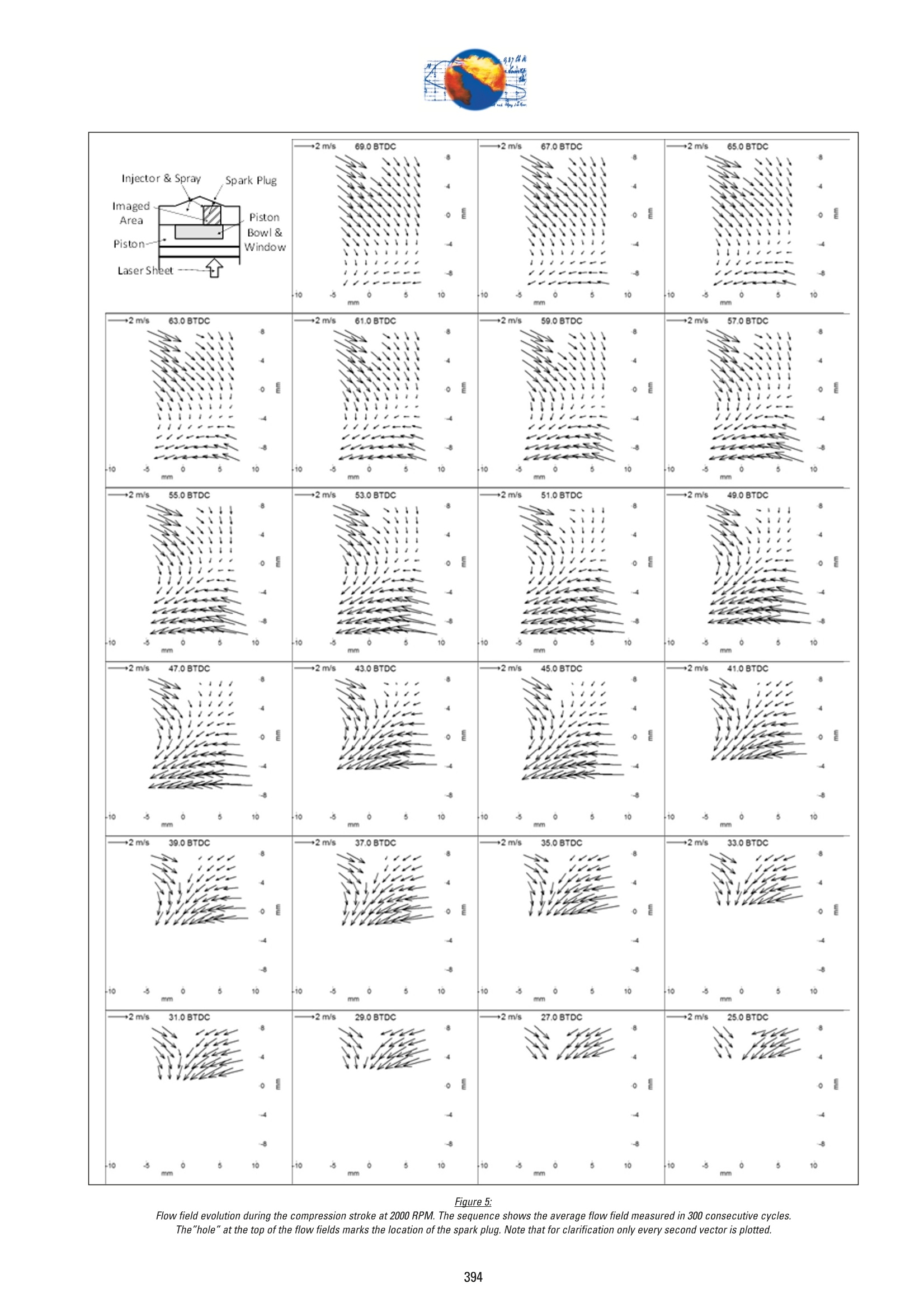
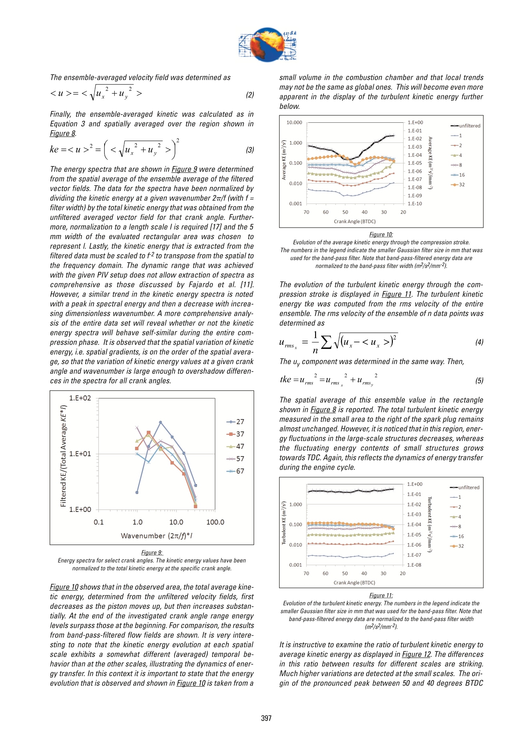
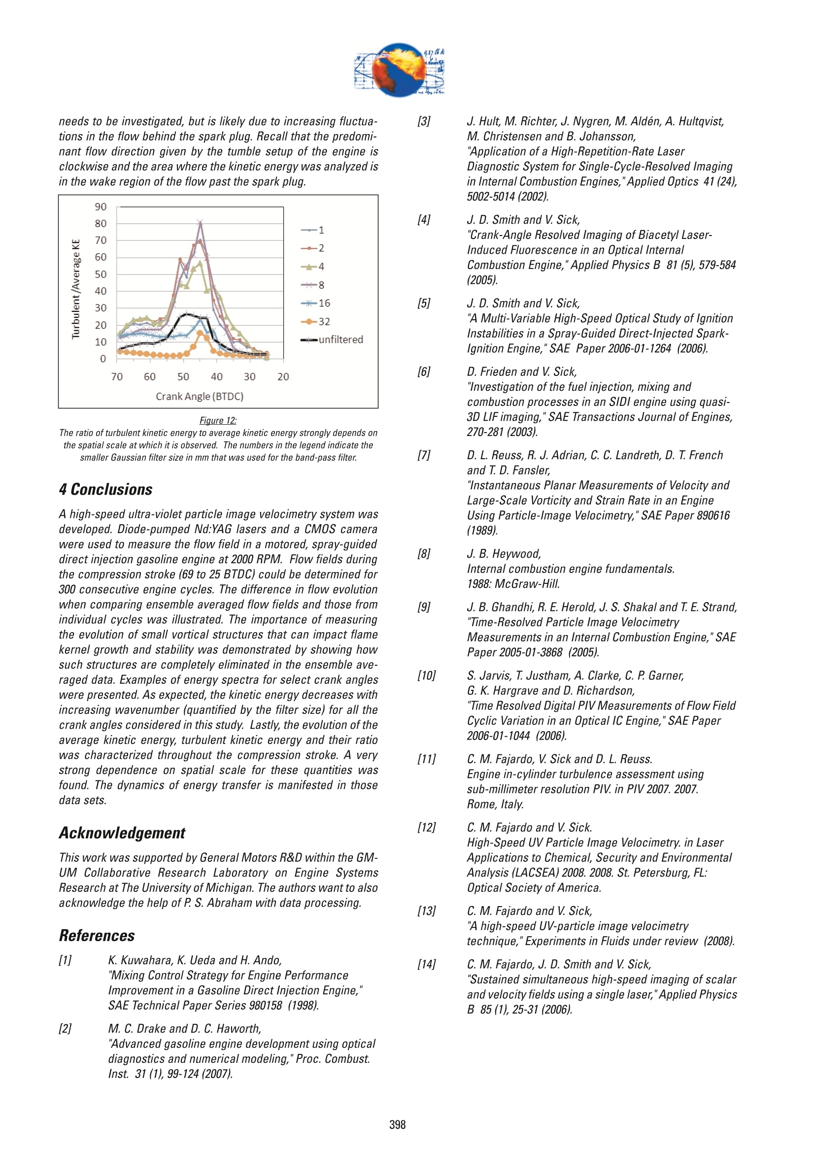
六人 ods儿a. Development and Applicationof High-Speed Imaging Diagnosticsfor Spray-Guided Spark-IgnitionDirect-Injection Engines Nn Prof. Dr. V. Sick The University of Michigan, Ann Arbor, USAProf. Dr. C. FajardoWestern Michigan University, Kalamazoo, USA Abstract Fuel/air mixing, in-cylinder flow, and spark discharge exhibitlarge cycle-to-cycle variations in internal combustion engines. Tofully understand how each of those parameters affects ignitionstability, it is necessary to measure them at high rate and in morethan one dimension. Imaging diagnostics, such as laser inducedfluorescence (LIF) for fuel concentration measurements and par-ticle image velocimetry (PIV), have been useful in engine rese-arch and development for almost two decades now. However,measurements were mostly restricted to one image per cycleand often not even in consecutive cycles. Very recently, the useof CMOS cameras, multi-stage image intensifiers, and highrepe-tition rate diode-pumped Nd:YAG lasers has allowed sustainedLIF imaging measurements at 12 kHz (= 1 crank angle degree at2000 RPM) for more than 1600 consecutive engine cycles. Thisapproach can be combined with PIV to yield simultaneous fueldistribution and velocity fields. Here we focus on the descriptionof some intricate details of the high-speed flow diagnostic deve-lopment and illustrate their use with examples obtained in aspray-guided spark-ignition direct-injection engine. 1 Introduction Improvements on internal combustion efficiency and reduction ofpollutant formation from the combustion process require thatengines be operated in combustion modes such as fuel direct-injection, staged combustion, and partially-premixed compres-sion ignition. This frequently means that combustion conditionsare being pushed towards stability limits, where small variationsin the fuel/air mixture or thermal conditions can lead to a signifi-cant increase in cycle-to-cycle fluctuations. Inherently, evenunder the best possible operating conditions internal combustionengines exhibit cycle-to-cycle fluctuations in all parameters (e.g.power, NOy, UBHC). The highly stratified fuel/air mixture distribu-tion during idle and light load operation in spray-guided direct-injection engines can lead to partial burns or even misfires andtherefore increase the cycle-to-cycle fluctuations significantly.Likewise, the highly diluted mixtures in premixed compressionignition engines can cause power and emissions fluctuations. Controlling the leading parameters that govern cycle-to-cyclefluctuations means that these parameters must first be identifiedand characterized. Optical imaging diagnostics have been usedin engine research and development for more than two decadesnow and have been instrumental in advancing engine technology[1]. The ability to directly observe the impact of fuel/air mixingandthe local flow on combustion, the spatial and temporaldetails of the formation of nitric oxide, and much more, has leadto a significantly improved understanding of internal combustionengines. With the availability of such data, the validation anddevelopment of computational tools has been accelerated [2]. Engine simulations using three-dimensional computational fluiddynamics are typically based on Reynolds-Averaged NavierStokes equation (RANS) approaches. Only recently, advances innumerical methods and computational power allow the imple-mentation of Large Eddy Simulations (LES) to internal combustionengine modeling. In combination with fast imaging technology,the use of LES modeling might provide insight into the nature ofcycle-to-cycle fluctuations, which currently limit improvementsin engine performance. The individual nature of each engine cycle requires that imagingmeasurements track the events within a single cycle. Therefore,image frame rates in the kHz range are needed to follow critical changes in the flow field and scalar quantities such as equiva-lence ratio or combustion progress. Until recently, it was not pos-sible to image equivalence ratio at such rates for more than eightimages per cycle, every few cycles [3]. Advances in solid statelasers and CMOS camera technology have recently allowed thedevelopment of a strategy to image equivalence ratio fields atcrank angle resolution for far more than 1000 consecutive enginecycles [4, 5]. Individual cycle behavior can now be tracked andthe role of local equivalence ratio on ignition stability can beassessed. This is especially important for spray-guided direct-injection engines, where the local equivalence ratio at the sparkplasma will vary greatly during the duration of the discharge. Even in the context of phase-averaged data that is conducive tosupport RANS-based modeling approaches, the availability ofhigh-speed imaging is welcome. As an example, data sets thatwere recorded in a matter of approximately 90 seconds [5] wouldrequire more than 30 hours of actual measurement time with atraditional laser/intensified camera system such as described byFrieden et al. [6]. An increased number of images is important toobtain a stable average that can be used for reliable computationof first and second moments of distributions. Not only do the cycle-to-cycle fluctuations in an engine require alarger number of data points for a stable average, but it is alsooften difficult to keep the operating conditions of optical enginesconstant over a longer period, thus potentially broadening thedistribution of measurement values. In regards to achieving astable average, note that depending on the nature of the velocityfluctuations, the average may actually be biased because it is notpossible to distinguish between turbulence and cycle-to-cyclefluctuations, since the latter are not part of the Reynolds decom-position approach. Just as important as the crank-angle-resolved measurement ofscalar fields is the characterization of the in-cylinder flow. Sinceparticle image velocimetry (PIV) was introduced to engine rese-arch [7], it has been applied in many different engines. As is thecase with phase-averaging of scalars, the RANS-based assess-ment of velocity data assumes that all fluctuations about a meanflow are attributed to turbulence. This creates uncertainty aboutthe origin and role of cycle-to-cycle fluctuations. Furthermore,combustion models that scale the flame speed with turbulenceproperties [8] might produce biased results. Lastly, the instant-aneous flow field and its development are crucial in assessingthe role of local and temporal changes of strain rate and vortici-ty on flame kernel growth and potential extinction. Averageddata are not useful in this context. As with high-speed scalarimaging, the availability of high-repetition rate lasers andcameras has allowed the development of high-speed PIV techni-ques. Laser pulse energies from high-repetition rate lasers arehigher in the visible and thus, such approaches have been ini-tially used [9, 10] in motored engines. The use of UV laser light isbeneficial when firing the engine because it helps to suppressthe recording of combustion luminosity. Single and dual lasersetups of UV-PIV systems have been demonstrated for engineresearch [11-13] under motored and fired engine operation. Anadditional advantage of UV-PIV is the option to simultaneouslyexcite LIF signals, for example to visualize a scalar distributionalong with the flow field measurement [14]. Here we focus on the description of high-speed velocity fieldmeasurements and present sample results from a spectral ana-lysis of velocity data that were obtained near the spark plug in aspray-guided direct-injection engine. 2 Experiment For PIV measurements, two exposures of particle scattering ima-ges need to be recorded at a known time delay. The time delaybetween the two scattering images from which a vector field iscomputed via cross-correlation depends on the velocity magnitu-de in the flow and the spatial resolution that is desired. For maxi-mum flexibility in adjusting the time delay, the use of two lasers isusually required. Two diode-pumped Nd:YAG lasers (QuantronixHawk /I-355M) were used for the measurements. The polariza-tion of one of the laser beams was rotated from vertical to hori-zontal to allow the overlap of both beams with minimized loss ofenergy in a beam splitter cube. The collinear beams were thenexpanded into a light sheet with a set of lenses. The light sheetwas aligned such that it entered the engine vertically via a tur-ning mirror that was placed inside the extended piston assembly.A plane parallel to the spark plug -fuel injector plane was illumi-nated..The light sheet was positioned approximately 2 mm infront of the spark electrodes, towards the side where the CMOScamera (Vision Research Phantom 7.3) recorded the Mie scatte-ring from the silicone oil droplets added to the intake air. A 70 mmdielectric mirror (CVI Lasers), coated for 355 nm, was used to iso Figure 1: Schematic setup of the dual laser UV-PIV system with frame-straddling CMOScamera. The optical components of the engine are shown only for clarity.The insert shows a photo of the transparent piston with side windowsin the piston bowl. Fiqure 2: Top view of the engine illustrating the size and location of the piston bowl, thespark plug, the injector and the light sheet arrangement. Note that the light sheetis located between the spark plug and the camera. late the Mie signals from other unwanted signals, such as fluore-scence. Signals were imaged onto the CMOS camera with a 105mm, fy=4.5, UV lens (Coastal Optics SLR). Figure 1 displays thesetup and laser sheet position in the engine. Figure 2 providesmore details on the location of the measurement plane within thecylinder. The camera and the lasers were synchronized to the engine'scrank shaft encoder. The engine speed was set to 2000 RPM andthe camera received a trigger every crank angle degree, i.e. atapproximately 12kHz. Each of the lasers fired every other crankangle (~6kHz) but at alternating camera frames so that a Miescattering imagewas acquiredatevery crankangle.Schematically, the timing is illustrated in Figure 3.17The enginewas motored at 2000 RPM, while the intake air was temperaturecontrolled to 45℃; the intake pressure was set at 95 kPa. Oil andcoolant temperatures were kept at 95℃. A summary of engineand PIV parameters is given in Table 1. Figure 3: Timing diagram showing the sequence of laser pulses and camera frame exposureduration and delay. The first laser pulse produces Mie scattering signals that arerecorded towards the end of the exposure of the first camera frame, the signalsfrom the second laser pulse are registered at the beginning of the next frame(=frame straddling). This way, pulse separation times and velocity range matchingfar better than given by the frame rate of the camera can be achieved. Table 1: Important engine and PIV settings. Parameter Value Lightsheet width 15mm Light sheet thickness 1mm Magnification ofimaging system 0.53 In-plane spatial resolution 1.4 mm Dynamic velocityrange 66:1 Maximum resolvable velocities 15m/s Spark plug J Fuel injector厂 8-hole Compression ratio 9:1 Engine speed 2000 RPM Intake temperature 45°C Intake pressure 95kPa The engine is a fully-trans-parentsingle cylinderengine with a pentrooffour-valve head. Both in-take ports were operatedfully open to minimizeswirl (swirl ratio ~0.8) butmaximize tumble (tumbleratio~0.7). Optical accessis provided through a fullquartz liner, a piston bot- tom window, piston bowl side windows and windows in the cylin-der head pentroof area (Fiqure 4). Figure 4:Photos of the optical engine. →2m/s 10 -5mm 69.0 BTDC8B4480 5 10 →2 m/s 67.0 BTDC 8 404-8B 10 5 10mm →2m/s 65.0 BTDC 8B 4 4 10 -85 5 10mm 一→2 m/s 63.0 BTDC8 ol 4 10 8B5 5 10mm *2 m/s 61.0 BTDC 8 oi 4 10 -5 0 5 10mm →2 m/s 59.0 BTDC 8 4 ol 4 8 10 0 5 10 mm *2 m/s 57.0BTDC 8 4 ol 4 10 -5 0 5 10mm →2m/s 55.0 BTDC 84 ol -10 0 5 10mm *2 m/s 53.0 BTDC 8B EE -10 -5 0 5 10mm -2m/s 51.0 BTDC 8 4 o 10mm kta5 0 5 10 →2m/s 47.0 BTDC84 -0 -8B -10 5 0 5 10mm +2 m/s 43.0 BTDC8 EE -8 10 -5 0 5 10mm →2 m/s 45.0 BTDC8 -8B 10 5 10mm +2 m/s E -8 10 -5 0 5 10mm →2 m/s 39.0 BTDC 8 4 8B 10 -5 0 5 10mm →2m/s 37.0 BTDC 8 -4 -8 10 -5 0 5 10mm →2m/s 35.0 BTDC 8 -4 8B 10 -5 5 10mm *2 m/s 33.0 BTDC ol -4 -8 10 -5 5 10mm -→2 m/s 31.0 BTDC 8 -4 -8B -10 5 0 5 10mm *2 m/s 29.0 BTDC -4 -8 10 -5 5 10mm →2 m/s 27.0 BTDC 4 -8 10 5 0 5 10mm +2m/s 25.0 BTDC ol -4 8 10 -5 0 5 10mm Figure 5: Flow field evolution during the compression stroke at 2000 RPM. The sequence shows the average flow field measured in 300 consecutive cycles. The"hole" at the top of the flow fields marks the location of the spark plug. Note that for clarification only every second vector is plotted. →2 m/s 65.0 BTDC a 4 →2m/s 63.0 BTDC ol -10 mm →2m/s 57.0 BTDC 4mm →2m/s 55.0 BTDC . al 4 4 10 →2m/s 53.0 BTDC →2 m/s 51.0 BTDC . 2 -10 →2m/s 49.0 BTDC 4 →2m/s 47.0 BTDC al 4 mn. →2m/s 45.0 BTDC →2m/s 43.0 BTDC →2m/s 41.0 BTDC . . . ma4 mm →2 m/s 39.0 BTDC 二 号 mm →2m/s 37.0 BTDC →2m/s 35.0 BTDC →2 m/s 33.0 BTDC. 2 mm4 →2m/s 31.0 BTDC 2 ol 4 →2m/s 29.0 BTDC →2m/s -. →2m/s 27.0 BTDC Figure 6: Evolution of the flow field in an individual cycle. Small vortical structures are visible that are convected with the flow field. The engine was motored at a steady speed of 2000 RPM and Miescattering images were recorded for 300 consecutive enginecycles for crank angles from 69 BTDC to 25 BTDC. The Mie scat-tering images were analyzed and processed with a cross-corre-lation algorithm (LaVision DaVis 7.1) and spatially filtered with a3x3 pixel filter to eliminate noise at the spatial resolution limit [11].The selected crank angle range is of particular interest becauseduring this time the fuel gets injected and ignited during low andpart-load operating conditions. Note that the discussion in thispaper focuses on motored, non-injection cases. To give an over-all impression of the flow in a plane parallel to the injector-sparkplug plane, a sequence of averaged flow fields is shown in Fiqure5. The clockwise tumble flow is very pronounced and persists in theimaged field of view until approximately 37 BTDC, when the flowis primarily directed towards the piston bowl. It is important tonote that the bottom location in the flow field shown in Figure 5and subsequent figures marks the top of the piston bowl sidewindows. With the settings used in the present study, the lensaperture was set for maximum light collection. As a result, thedepth of focus was very short and image distortions through thethick side windows did not allow focused imaging of the Miescattering signals [15]. A set of flow fields from a randomly chosen cycle (#4 of 300) isdisplayed in Figure 6 to illustrate how different the instantaneousflow pattern evolves in comparison to the averaged flow field.While overall the tumble structure of the average flow field asseen in Fiqure 5 underlies the instantaneous flow fields, there arepronounced differences that cannot be captured from an exami-nation of the averages. An example is the small vortical structu-re that appears at 57 BTDC on the left side of the flow field at aheight of 0 mm. This structure moves approximately horizontallybefore it is dissipated or has moved away in the third dimension.The diameter of this vortex is approximately 3-4 mm and thus of adimension that is comparable too an early flame kernel.Interactions between such vortices and early flame kernelscould lead to extinction. It is therefore important to have indivi-dual-cycle flow field sequences available to study flame initia-tion, growth, and extinction. The random nature of the timing andlocation of such small structures leads to their elimination in theaverage flow field, and any role that they might play in influencingcombustion is lost in the average data set. Flow structures of different size and energy content will havedifferent influence on ignition, flame kernel development andflame speed. The structure and energy contents of the flow wereexamined after applying a 2D-Gaussian band-pass filter [7, 11]. Toaccomplish this, the instantaneous velocity fields were filteredwith Gaussian low-pass filters of sizes chosen such that the dif-ference between neighboring filters produced a constant band-width filter in wavenumber space. This width was set to 0.001mm-1.The width of the smaller of the neighboring filters is used inthis paper to denote the flow fields that are calculated with theband-pass filters. The larger the filter size, the more closely theresulting vector field resembles the ensemble averaged flowfield [16]. Figure Z shows the band-pass-filtered flow field for 41BTDC from the sequence that is displayed in Figure 6. Fiqure 7: Flow field at 41 BTDC from the cycle shown in Figure 6. The original flow field wass1ISpatially filtered with a 2D-Gaussian filter. Combinations of filtered flow fields werecomputed to produce band-pass-filtered flow fields as shown here. The dimensions given in the vector fields are the 1/e2 width of the smaller of theGaussian filters that were used for the corresponding band-pass. Note that thelength of the vector displays is not constant across all figures. The first image shows the instantaneous unfiltered flow field forcomparison. The largest filter used has an f=1/e2-width of 32 mmand the resulting vector field is very similar to the ensemble ave-rage (compare to Figure 5). With decreasing width of theGaussian filters, more small-scale structures are unveiled. Forexample, the vortex to the right of the spark plug is not present inthe 32 mm filtered flow field but begins to appear at 16 mm andbelow. At the smallest filter sizes, the flow is more random. Theflow decomposition with the band-pass filters allows the identifi-cation of prominent structures and their evolution. As such, thiswill be a useful method to isolate flow structures that have adominating impact on e. g. flame kernel extinction. It is also apparent from the vector fields shown in Figure Z thatthe velocity magnitude in the narrow band passes decreaseswith decreasing filter size, reflecting a decrease in kineticenergy contents at this particular scale. INote also that theimpact of a spatially finite flow field may introduce less accuratevelocity vectors at the edges of the filtered flow fields. This isapparent in the examples for smallest filter sizes shown in Figure7. A small area to the right of the spark plug,downstream of the fueljet that impacts the spark electrodes when fuel is injected, waschosen for this study to examine the evolution of the kinetic ener-gy ke over a range of crank angles and spatial scales. Figure 8shows the location of the area for which the spatially averagedkinetic energy was computed. The ensemble-averaged velocity field was determined as Finally, the ensemble-averaged kinetic was calculated as inEquation 3 and spatially averaged over the region shown inFigure 8. The energy spectra that are shown in Figure 9 were determinedfrom the spatial average of the ensemble average of the filteredvector fields. The data for the spectra have been normalized bydividing the kinetic energy at a given wavenumber 2m/f (with f=filter width) by the total kinetic energy that was obtained from theunfiltered averaged vector field for that crank angle. Further-more, normalization to a length scale l is required [17] and the 5mm width of the evaluated rectangular area was chosentorepresent l. Lastly, the kinetic energy that is extracted from thefiltered data must be scaled to f2 to transpose from the spatial tothe frequency domain. The dynamic range that was achievedwith the given PIV setup does not allow extraction of spectra ascomprehensive as those discussed by Fajardo et al. [11].However, a similar trend in the kinetic energy spectra is notedwith a peak in spectral energy and then a decrease with increa-sing dimensionless wavenumber. A more comprehensive analy-sis of the entire data set will reveal whether or not the kineticenergy spectra will behave self-similar during the entire com-pression phase. It is observed that the spatial variation of kineticenergy, i.e.spatial gradients, is on the order of the spatial avera-ge, so that the variation of kinetic energy values at a given crankangleand wavenumber is large enough to overshadow differen-ces in the spectra for all crank angles. Figure9: Energy spectra for select crank angles. The kinetic energy values have beennormalized to the total kinetic energy at the specific crank angle. Figure 10 shows that in the observed area, the total average kine-tic energy,determined from the unfiltered velocity fields, firstdecreases as the piston moves up, but then increases substan-tially. At the end of the investigated crank angle range energylevels surpass those at the beginning. For comparison, the resultsfrom band-pass-filtered flow fields are shown. It is very intere-sting to note that the kinetic energy evolution at each spatialscale exhibits a somewhat different (averaged) temporal be-havior than at the other scales, illustrating the dynamics of ener-gy transfer. In this context it is important to state that the energyevolution that is observed and shown in Figure 10 is taken from a small volume in the combustion chamber and that local trendsmay not be the same as global ones. This will become even moreapparent in the display of the turbulent kinetic energy furtherbelow. Figure 10: Evolution of the average kinetic energy through the compression stroke.The numbers in the legend indicate the smaller Gaussian filter size in mm that wasused for the band-pass filter. Note that band-pass-filtered energy data arenormalized to the band-pass filter width (m²/s2/mm2). The evolution of the turbulent kinetic energy through the com-pression stroke is displayed in Figure 11. The turbulent kineticenergy tke was computed from the rms velocity of the entireensemble. The rms velocity of the ensemble of n data points wasdetermined as The uy component was determined in the same way. Then, The spatial average of this ensemble value in the rectangleshown in Figure 8 is reported. The total turbulent kinetic energymeasured in the small area to the right of the spark plug remainsalmost unchanged. However, it is noticed that in this region, ener-gy fluctuations in the large-scale structures decreases, whereasthe fluctuating energy contents of small structures growstowards TDC. Again, this reflects the dynamics ofenergy transferduring the engine cycle. Figure11: Evolution of the turbulent kinetic energy. The numbers in the legend indicate thesmaller Gaussian filter size in mm that was used for the band-pass filter. Note thatband-pass-filtered energy data are normalized to the band-pass filter width(m2/s2/mm-2). It is instructive to examine the ratio of turbulent kinetic energy toaverage kinetic energy as displayed in Figure 12. The differencesin this ratio between results for different scales are striking.Much higher variations are detected at the small scales. The ori-gin of the pronounced peak between 50 and 40 degrees BTDC needs to be investigated, but is likely due to increasing fluctua-tions in the flow behind the spark plug. Recall that the predomi-nant flow direction given by the tumble setup of the engine isclockwise and the area where the kinetic energy was analyzed isin the wake region of the flow past the spark plug. Figure12: The ratio of turbulent kinetic energy to average kinetic energy strongly depends onthe spatial scale at which it is observed. The numbers in the legend indicate thesmaller Gaussian filter size in mm that was used for the band-pass filter. 4 Conclusions A high-speed ultra-violet particle image velocimetry system wasdeveloped. Diode-pumped Nd:YAG lasers and a CMOS camerawere used to measure the flow field in a motored, spray-guideddirect injection gasoline engine at 2000 RPM. Flow fields duringthe compression stroke (69 to 25 BTDC) could be determined for300 consecutive engine cycles. The difference in flow evolutionwhen comparing ensemble averaged flow fields and those fromindividual cycles was illustrated. The importance of measuringthe evolution of small vortical structures that can impact flamekernel growth and stability was demonstrated by showing howsuch structures are completely eliminated in the ensemble ave-raged data. Examples of energy spectra for select crank angleswere presented. As expected, the kinetic energy decreases withincreasing wavenumber (quantified by the filter size) for all thecrank angles considered in this study. Lastly,the evolution of theaverage kinetic energy, turbulent kinetic energy and their ratiowas characterized throughout the compression stroke. A verystrong dependence on spatial scale for these quantities wasfound. The dynamics of energy transfer is manifested in thosedata sets. Acknowledgement This work was supported by General Motors R&D within the GM-UM Collaborative Research Laboratory on Engine SystemsResearch at The University of Michigan.The authors want to alsoacknowledge the help of P.S. Abraham with data processing. References [1] K. Kuwahara, K. Ueda and H. Ando,"Mixing Control Strategy for Engine PerformanceImprovement in a Gasoline Direct Injection Engine,"SAE Technical Paper Series 980158 (1998). [2] M. C. Drake and D. C. Haworth,"Advanced gasoline engine development using opticaldiagnostics and numerical modeling,"Proc. Combust.Inst. 31(1),99-124(2007). [3] J. Hult, M. Richter, J. Nygren, M. Alden, A. Hultqvist,M.Christensen and B. Johansson,"Application of a High-Repetition-Rate LaserDiagnostic System for Single-Cycle-Resolved Imagingin Internal Combustion Engines,"Applied Optics 41 (24),5002-5014(2002). [4] J. D. Smith and V. Sick. "Crank-Angle Resolved Imaging of Biacety/ Laser-Induced Fluorescence in an Optical InternalCombustion Engine,"Applied Physics B 81 (5), 579-584(2005). [5] J. D. Smith and V. Sick."A Multi-Variable High-Speed Optical Study of IgnitionInstabilities in a Spray-Guided Direct-Injected Spark-Ignition Engine,"SAE Paper 2006-01-1264 (2006). [6] D. Frieden and V. Sick,"Investigation of the fuel injection, mixing andcombustion processes in an SIDl engine using quasi-3D LIF imaging," SAE Transactions Journal of Engines,270-281 (2003). [7] D. L. Reuss, R. J. Adrian, C. C. Landreth, D. T. Frenchand T. D. Fansler."Instantaneous Planar Measurements of Velocity andLarge-Scale Vorticity and Strain Rate in an EngineUsing Particle-Image Velocimetry,"SAE Paper 890616(1989). [8] J. B.Heywood,Internal combustion engine fundamentals.1988: McGraw-Hill. [9] J.B. Ghandhi, R. E. Herold,J. S. Shakal and T. E. Strand,"Time-Resolved Particle Image VelocimetryMeasurements in an Internal Combustion Engine,"SAEPaper 2005-01-3868 (2005). [10] S. Jarvis, T. Justham, A. Clarke, C. P. Garner,G. K. Hargrave and D.Richardson,"Time Resolved Digital P/V Measurements of Flow FieldCyclic Variation in an Optical IC Engine,"SAE Paper2006-01-1044 (2006). [11] C. M. Fajardo, V. Sick and D. L. Reuss.Engine in-cylinder turbulence assessment usingsub-millimeter resolution PIV. in PIV 2007. 2007.Rome, Italy. ( [12] C. M. Fajardo and V . S ick. High-Speed UV Particle Image Velocimetry. in LaserApplications to Chemical, Security and EnvironmentalAnalysis (LACSEA) 2008. 2008. St. Petersburg, FL: Optical Society of America. ) [13] C. M. Fajardo and V. Sick,"A high-speed UV-particle image velocimetrytechnique,"Experiments in Fluids under review (2008). [14] C. M. Fajardo, J.D. Smith and V. Sick,"Sustained simultaneous high-speed imaging of scalarand velocity fields using a single laser,"Applied PhysicsB 85(1),25-31(2006). /15/ M. Megerle, V.Sick and D. L. Reuss,"Measurement of Digital P/V Precision usingElectrooptically-Created Particle-ImageDisplacements,"Measurement Science andTechnology 13, 997-1005(2002). D. L. Reuss, "Cyclic Variability of Large-Scale Turbulent Structures in Directed and Undirected IC Engine Flows," SAE Paper 2000-01-0246 (2000). /17/ H. Tennekes and J. L. Lumley, A First Course in Turbulence. 1972, Cambridge, MA: The MIT Press. Fuel/air mixing, in-cylinder flow, and spark discharge exhibitlarge cycle-to-cycle variations in internal combustion engines. Tofully understand how each of those parameters affects ignitionstability, it is necessary to measure them at high rate and in morethan one dimension. Imaging diagnostics, such as laser inducedfluorescence (LIF) for fuel concentration measurements and particleimage velocimetry (PIV), have been useful in engine researchand development for almost two decades now. However,measurements were mostly restricted to one image per cycleand often not even in consecutive cycles. Very recently, the useof CMOS cameras, multi-stage image intensifiers, and high repetitionrate diode-pumped Nd:YAG lasers has allowed sustainedLIF imaging measurements at 12 kHz (= 1 crank angle degree at2000 RPM) for more than 1600 consecutive engine cycles. Thisapproach can be combined with PIV to yield simultaneous fueldistribution and velocity fields. Here we focus on the descriptionof some intricate details of the high-speed flow diagnostic developmentand illustrate their use with examples obtained in aspray-guided spark-ignition direct-injection engine.
确定


还剩7页未读,是否继续阅读?

产品配置单

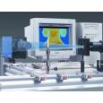

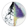
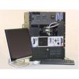
北京欧兰科技发展有限公司为您提供《喷雾导引火花塞引燃直接喷射发动机(SGSIDI)中高速成像诊断检测方案(粒子图像测速)》,该方案主要用于汽车电子电器中理化分析检测,参考标准--,《喷雾导引火花塞引燃直接喷射发动机(SGSIDI)中高速成像诊断检测方案(粒子图像测速)》用到的仪器有德国LaVision PIV/PLIF粒子成像测速场仪、PLIF平面激光诱导荧光火焰燃烧检测系统、LaVision HighSpeedStar 高帧频相机、LaVision SprayMaster 喷雾成像测量系统、汽车发动机多参量测试系统
推荐专场


相关方案
更多
该厂商其他方案
更多