


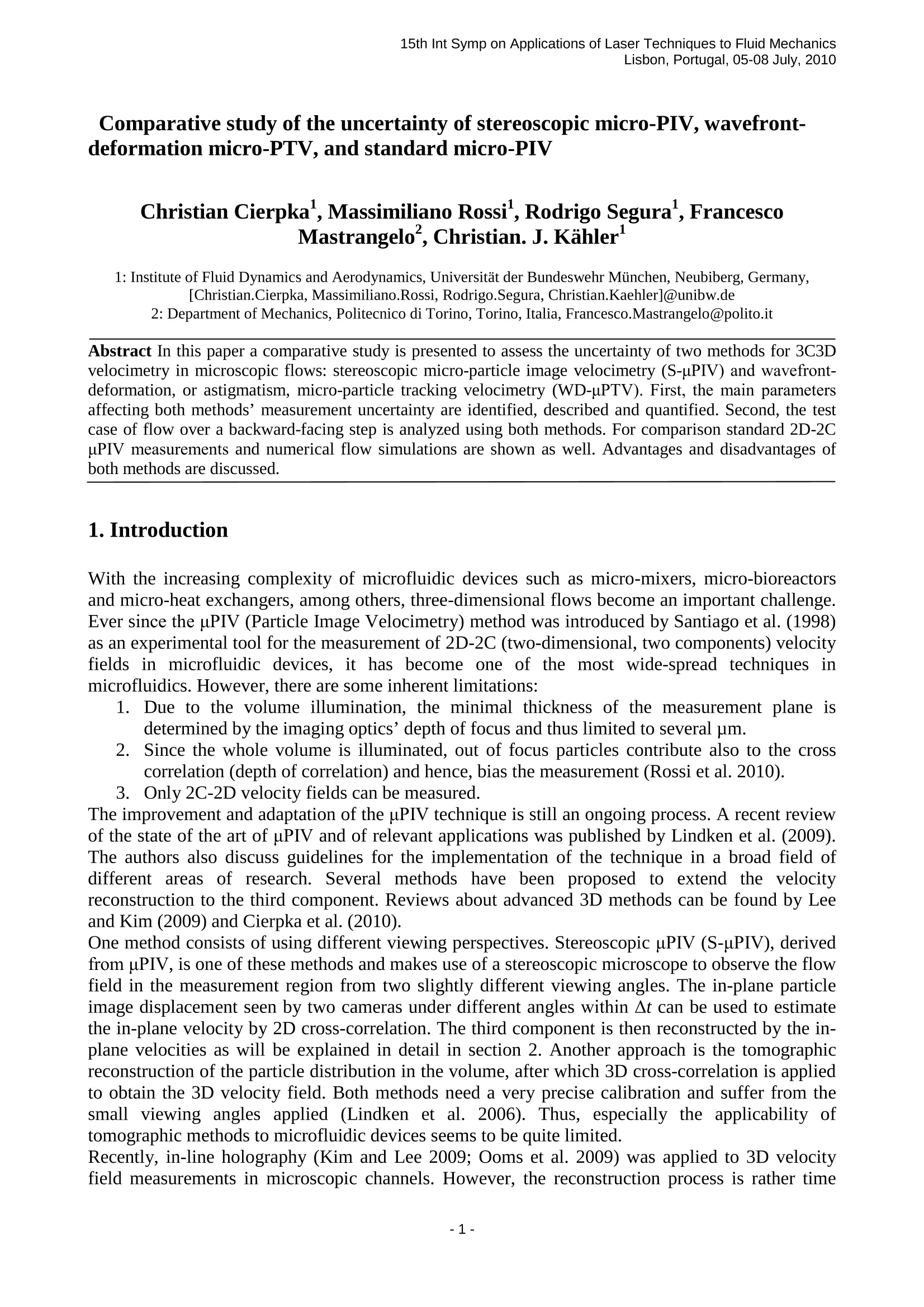
In this paper a comparative study is presented to assess the uncertainty of two methods for 3C3D velocimetry in microscopic flows: stereoscopic micro-particle image velocimetry (S-μPIV) and wavefront-deformation, or astigmatism, micro-particle tracking velocimetry (WD-μPTV). First, the main parameters affecting both methods’ measurement uncertainty are identified, described and quantified. Second, the test case of flow over a backward-facing step is analyzed using both methods. For comparison standard 2D-2C μPIV measurements and numerical flow simulations are shown as well. Advantages and disadvantages of both methods are discussed.
方案详情

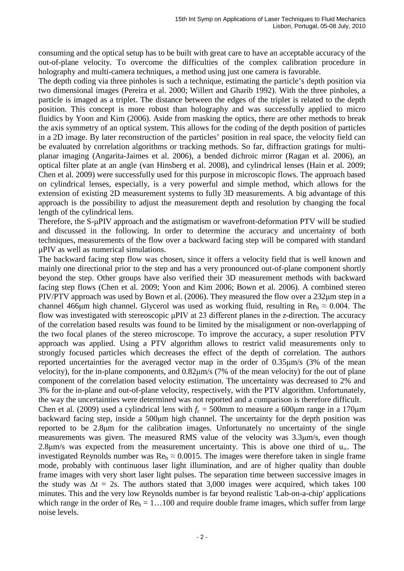
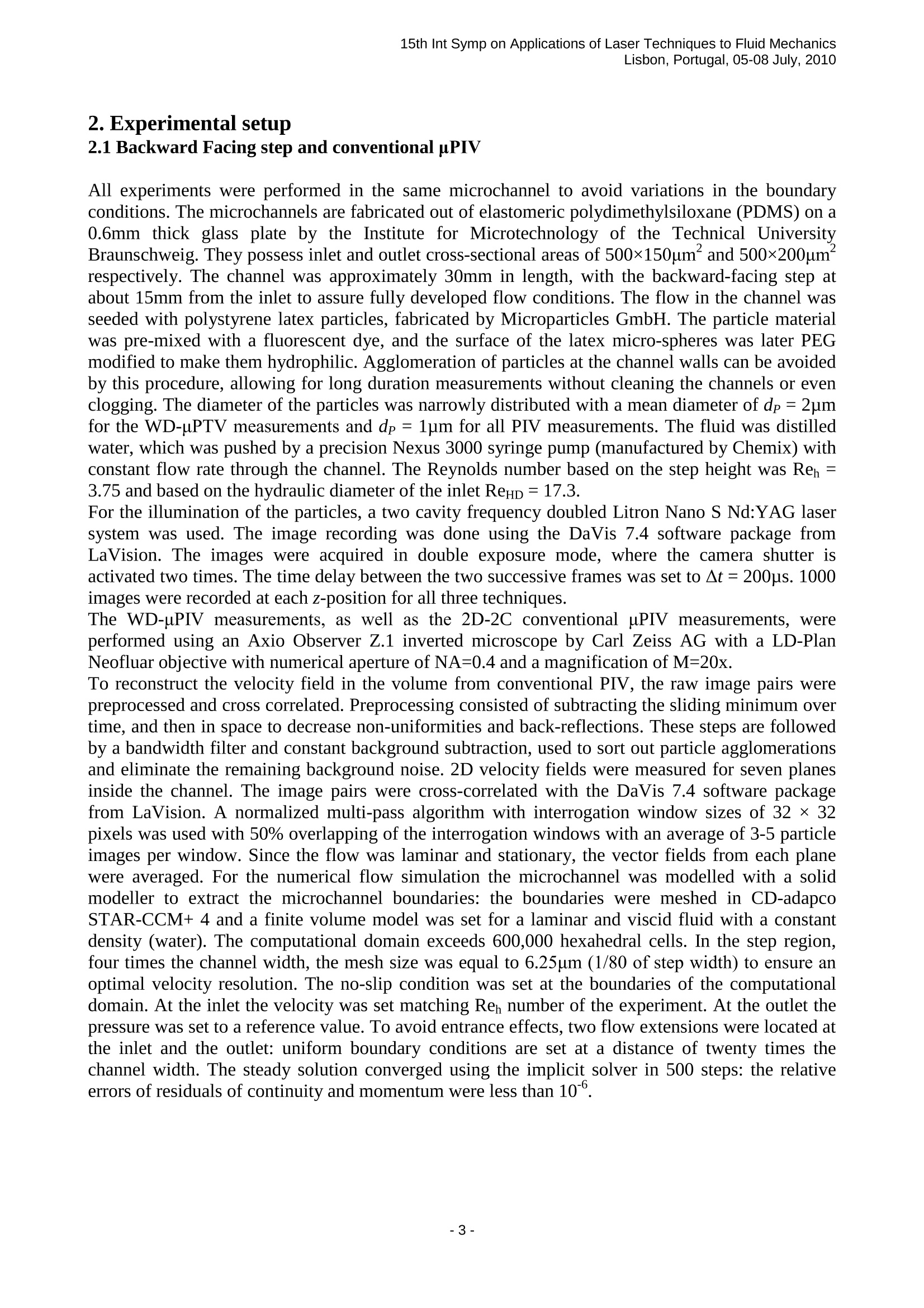
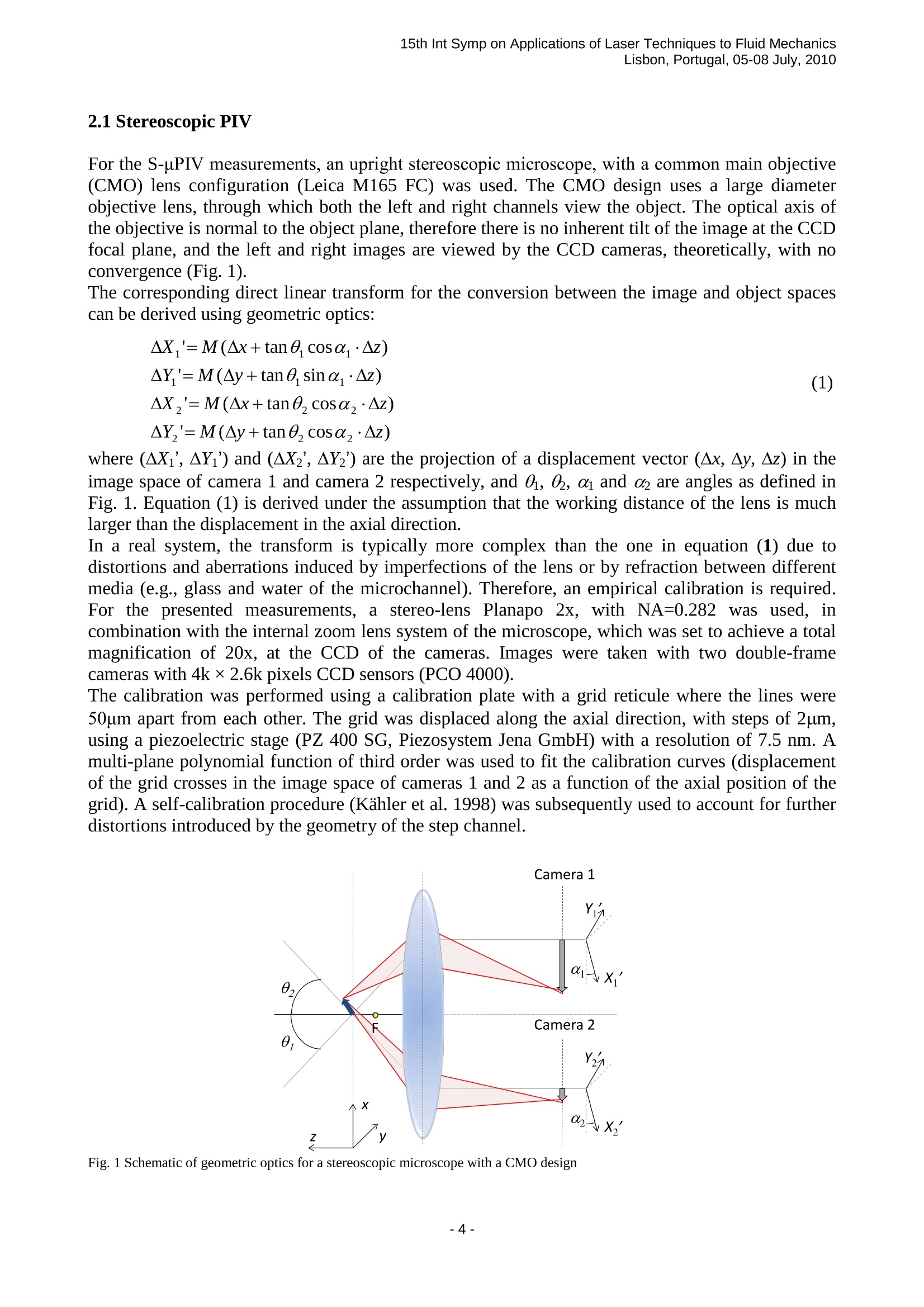
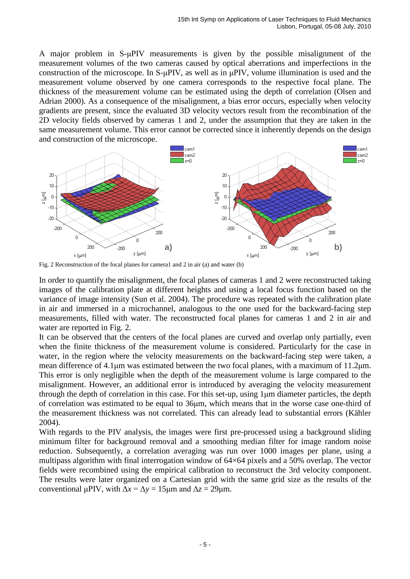
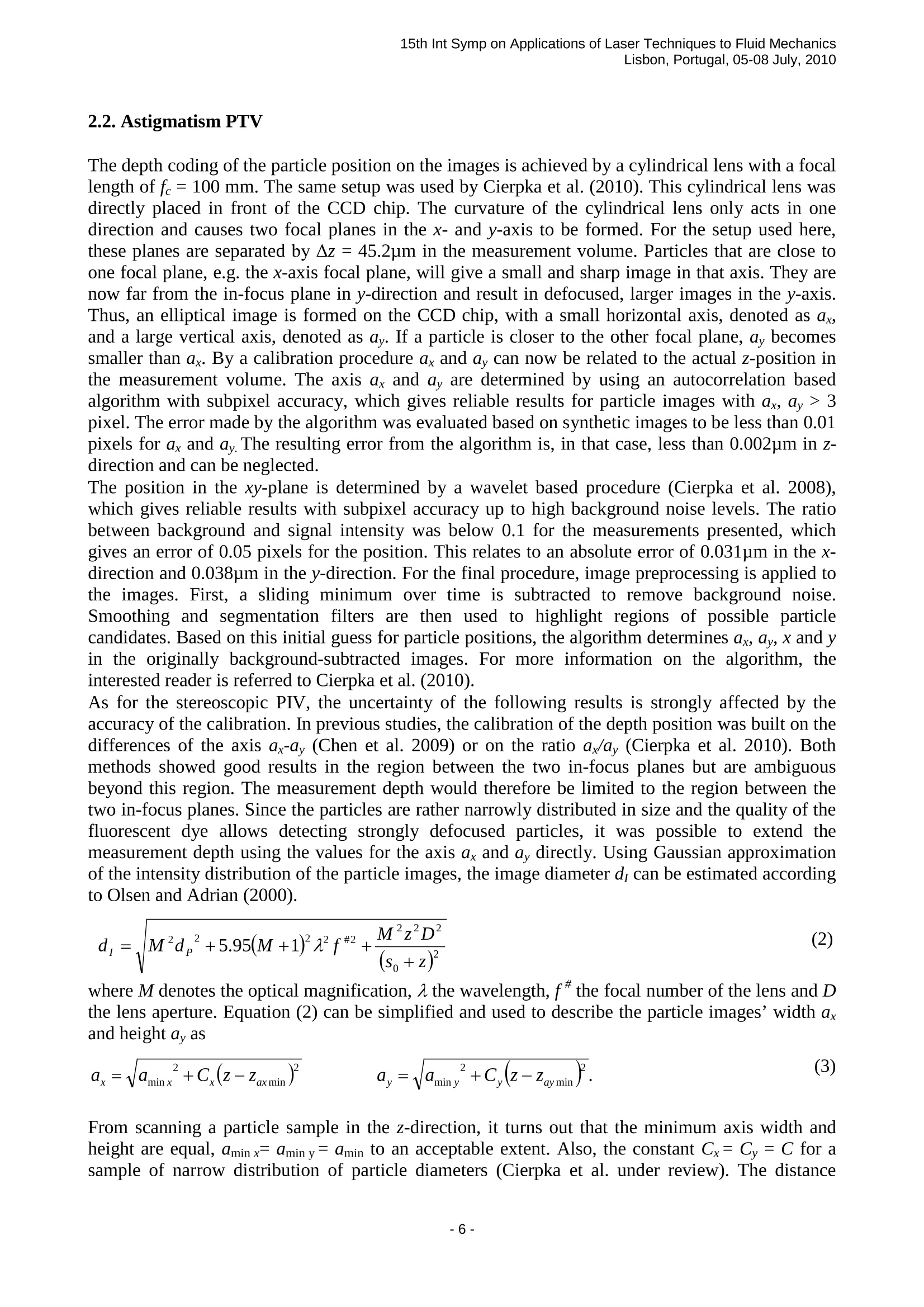
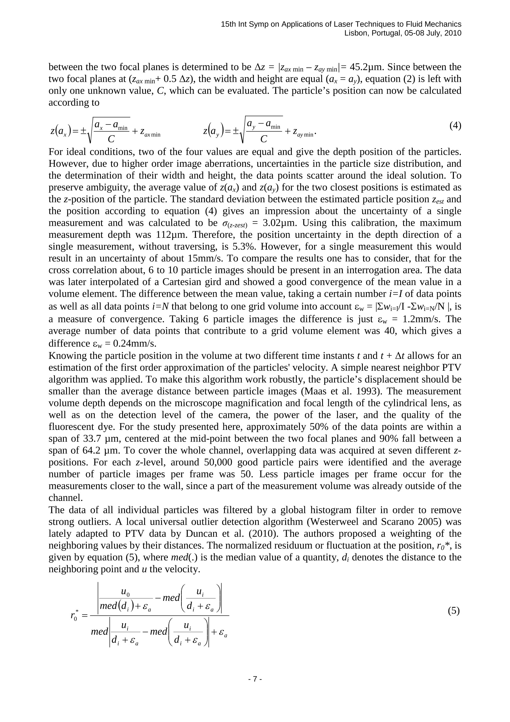
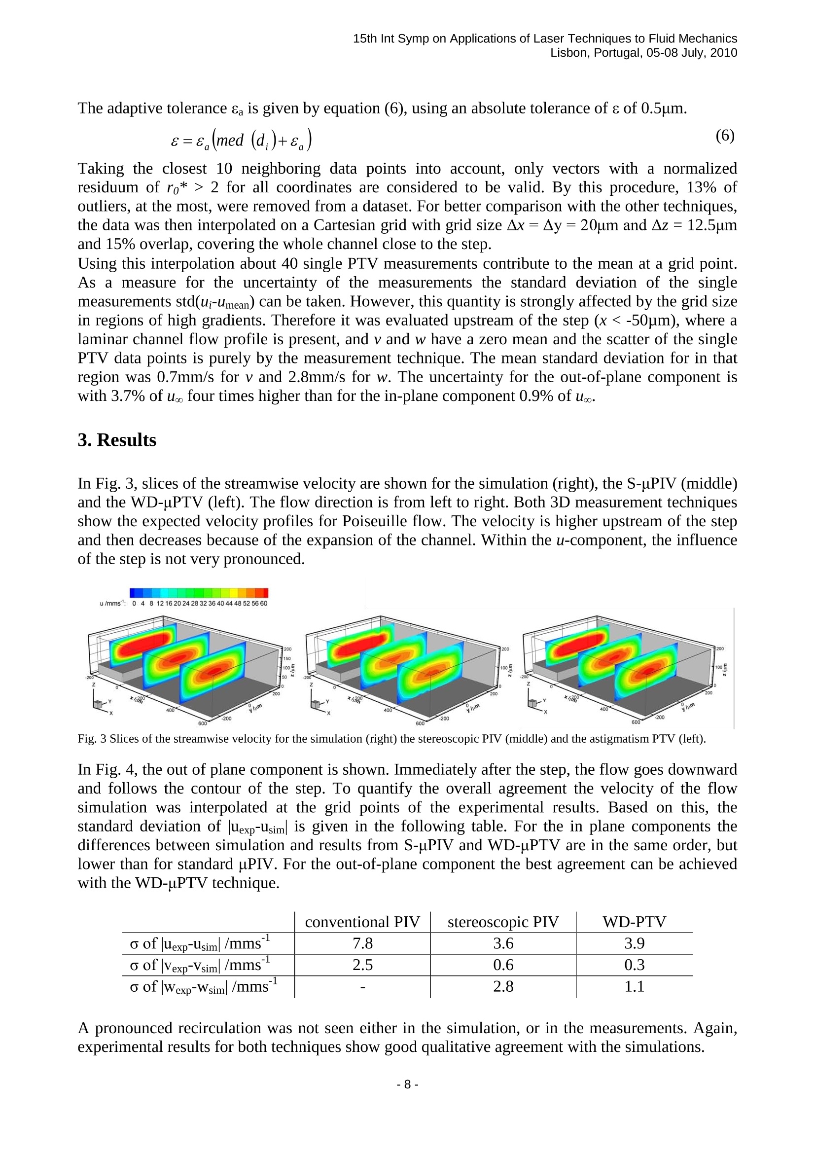
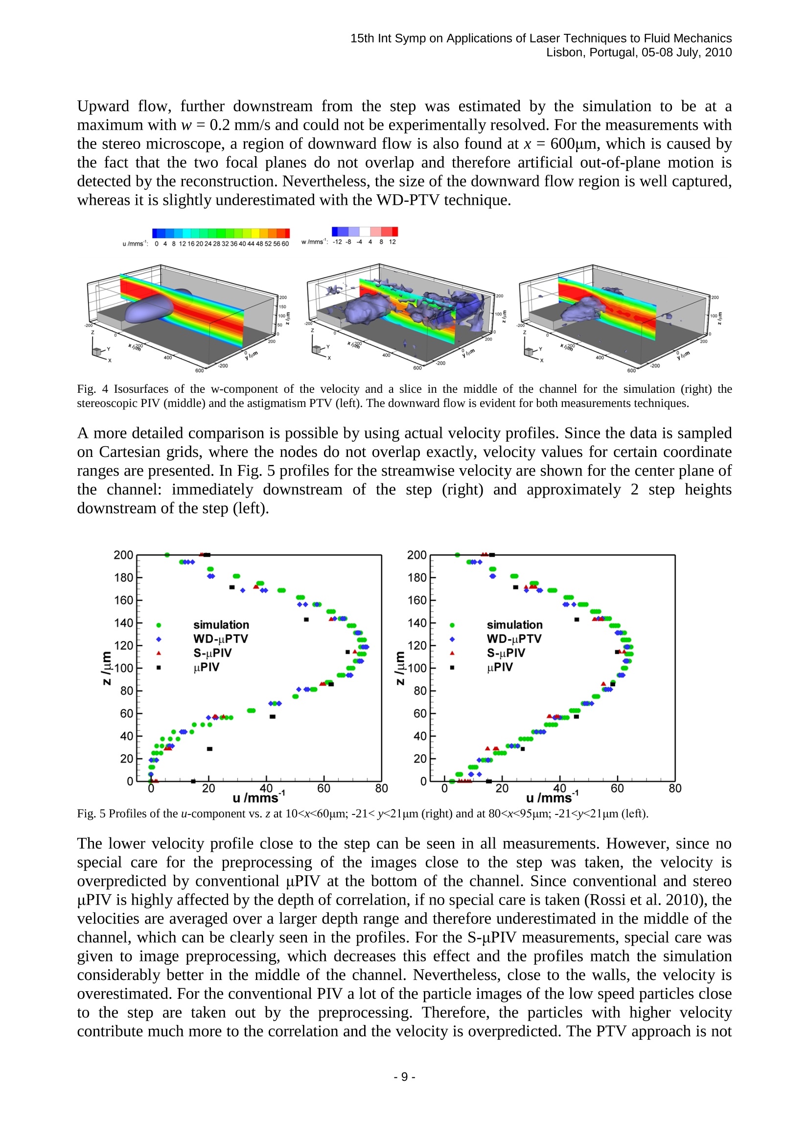
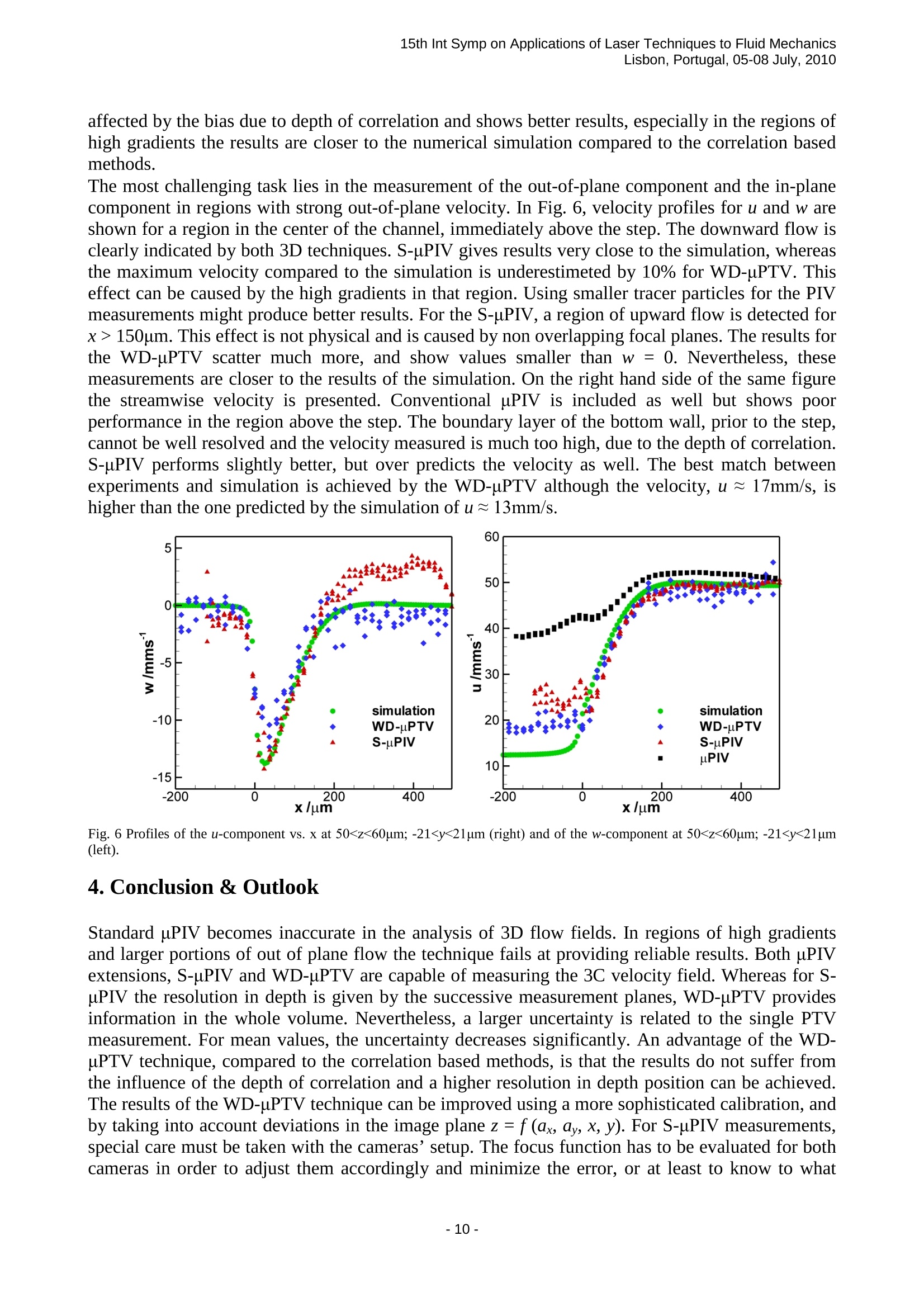
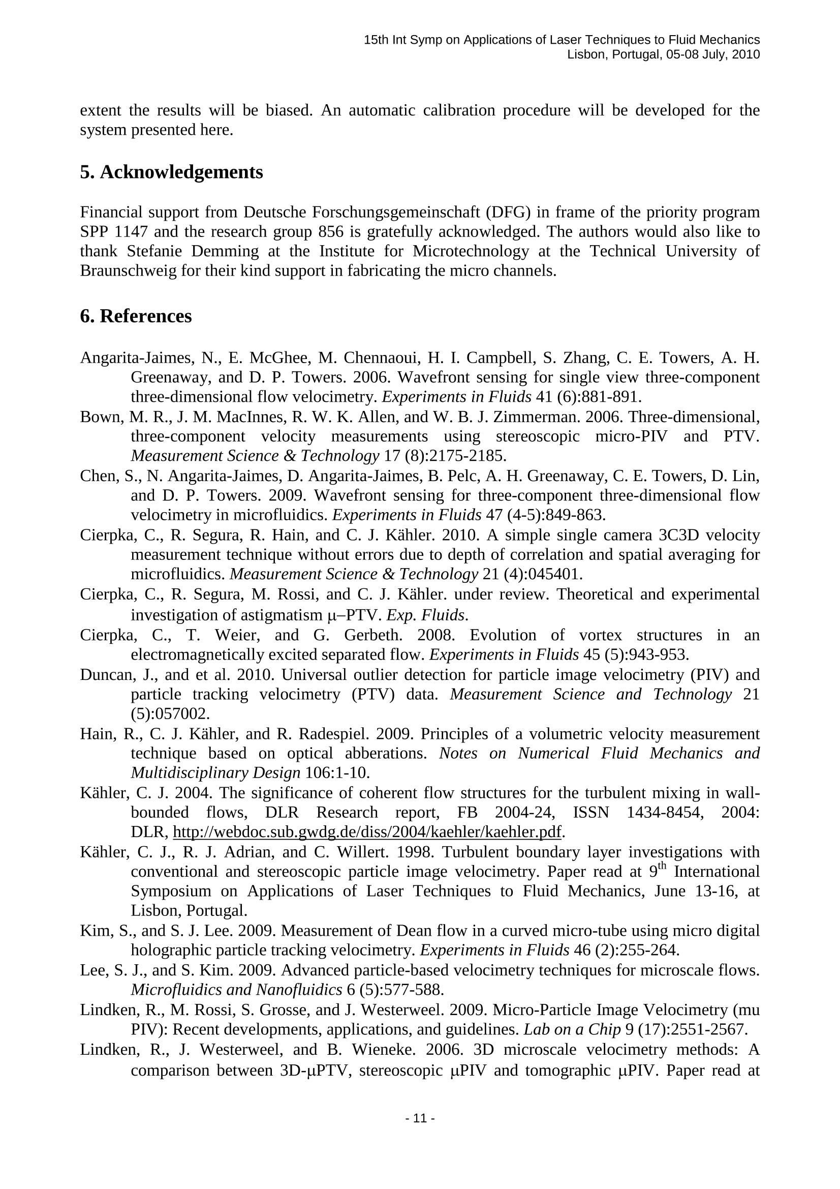
15th Int Symp on Applications of Laser Techniques to Fluid MechanicsLisbon, Portugal, 05-08 July,2010 Comparative study of the uncertainty of stereoscopic micro-PIV, wavefront-deformation micro-PTV, and standard micro-PIV Christian Cierpka', Massimiliano Rossi , Rodrigo Segura', FrancescoMastrangelo, Christian. J. Kahler 1: Institute of Fluid Dynamics and Aerodynamics, Universitat der Bundeswehr Munchen, Neubiberg, Germany, [Christian.Cierpka, Massimiliano.Rossi, Rodrigo.Segura, Christian.Kaehler]@unibw.de 2: Department of Mechanics, Politecnico di Torino, Torino, Italia, Francesco.Mastrangelo@polito.it Abstract In this paper a comparative study is presented to assess the uncertainty of two methods for 3C3Dvelocimetry in microscopic flows: stereoscopic micro-particle image velocimetry (S-uPIV) and wavefront-deformation, or astigmatism, micro-particle tracking velocimetry (WD-uPTV). First, the main parametersaffecting both methods’measurement uncertainty are identified, described and quantified. Second, the testcase of flow over a backward-facing step is analyzed using both methods. For comparison standard 2D-2CuPIV measurements and numerical flow simulations are shown as well. Advantages and disadvantages ofboth methods are discussed. 1. Introduction With the increasing complexity of microfluidic devices such as micro-mixers, micro-bioreactorsand micro-heat exchangers, among others, three-dimensional flows become an important challenge.Ever since the uPIV (Particle Image Velocimetry) method was introduced by Santiago et al. (1998)as an experimental tool for the measurement of 2D-2C (two-dimensional, two components) velocityfields in microfluidic devices, it has become one of the most wide-spread techniquesmicrofluidics. However, there are some inherent limitations: 1. Due to the volume illumination, the minimal thickness of the measurement plane isdetermined by the imaging optics’depth of focus and thus limited to several um. 2. SSince the whole volume is illuminated, out of focus particles contribute also to the crosscorrelation (depth of correlation) and hence, bias the measurement (Rossi et al. 2010). 3. Only 2C-2D velocity fields can be measured. The improvement and adaptation of the uPIV technique is still an ongoing process. A recent reviewof the state of the art of uPIV and of relevant applications was published by Lindken et al. (2009).The authors also discuss guidelines for the implementation of the technique in a broad field ofdifferent areas of research. Several methods have been proposed to extend the velocityreconstruction to the third component. Reviews about advanced 3D methods can be found by Leeand Kim (2009) and Cierpka et al. (2010). One method consists of using different viewing perspectives. Stereoscopic pPIV (S-pPIV), derivedfrom uPIV, is one of these methods and makes use of a stereoscopic microscope to observe the flowfield in the measurement region from two slightly different viewing angles. The in-plane particleimage displacement seen by two cameras under different angles within At can be used to estimatethe in-plane velocity by 2D cross-correlation. The third component is then reconstructed by the in-plane velocities as will be explained in detail in section 2. Another approach is the tomographicreconstruction of the particle distribution in the volume, after which 3D cross-correlation is appliedto obtain the 3D velocity field. Both methods need a very precise calibration and suffer from thesmall viewing angles applied (Lindken et al. 2006). Thus, especially the applicability oftomographic methods to microfluidic devices seems to be quite limited. Recently, in-line holography (Kim and Lee 2009; Ooms et al. 2009) was applied to 3D velocityfield measurements in microscopic channels. However, the reconstruction process is rather time consuming and the optical setup has to be built with great care to have an acceptable accuracy of theout-of-plane velocity. To overcome the difficulties of the complex calibration procedure inholography and multi-camera techniques,a method using just one camera is favorable. The depth coding via three pinholes is such a technique, estimating the particle’s depth position viatwo dimensional images (Pereira et al. 2000; Willert and Gharib 1992). With the three pinholes, aparticle is imaged as a triplet. The distance between the edges of the triplet is related to the depthposition. This concept is more robust than holography and was successfully applied to microfluidics by Yoon and Kim (2006). Aside from masking the optics, there are other methods to breakthe axis symmetry of an optical system. This allows for the coding of the depth position of particlesin a2D image. By later reconstruction of the particles’ position in real space, the velocity field canbe evaluated by correlation algorithms or tracking methods. So far, diffraction gratings for multi-planar imaging (Angarita-Jaimes et al. 2006), a bended dichroic mirror (Ragan et al. 2006), anoptical filter plate at an angle (van Hinsberg et al.2008), and cylindrical lenses (Hain et al. 2009;Chen et al. 2009) were successfully used for this purpose in microscopic flows. The approach basedon cylindrical lenses, especially, is a very powerful and simple method, which allows for theextension of existing 2D measurement systems to fully 3D measurements. A big advantage of thisapproach is the possibility to adjust the measurement depth and resolution by changing the focallength of the cylindrical lens. Therefore, the S-uPIV approach and the astigmatism or wavefront-deformation PTV will be studiedand discussed in the following. In order to determine the accuracy and uncertainty of bothtechniques, measurements of the flow over a backward facing step will be compared with standarduPIV as well as numerical simulations. The backward facing step flow was chosen, since it offers a velocity field that is well known andmainly one directional prior to the step and has a very pronounced out-of-plane component shortlybeyond the step. Other groups have also verified their 3D measurement methods with backwardfacing step flows (Chen et al. 2009; Yoon and Kim 2006; Bown et al. 2006). A combined stereoPIV/PTV approach was used by Bown et al. (2006). They measured the flow over a 232um step in achannel 466um high channel. Glycerol was used as working fluid, resulting in Reh ~0.004. Theflow was investigated with stereoscopic uPIV at 23 different planes in the z-direction. The accuracyof the correlation based results was found to be limited by the misalignment or non-overlapping ofthe two focal planes of the stereo microscope. To improve the accuracy, a super resolution PTVapproach was applied. Using a PTV algorithm allows to restrict valid measurements only tostrongly focused particles which decreases the effect of the depth of correlation. The authorsreported uncertainties for the averaged vector map in the order of 0.35um/s (3% of the meanvelocity), for the in-plane components, and 0.82um/s (7% of the mean velocity) for the out of planecomponent of the correlation based velocity estimation. The uncertainty was decreased to 2% and3% for the in-plane and out-of-plane velocity, respectively, with the PTV algorithm. Unfortunately,the way the uncertainties were determined was not reported and a comparison is therefore difficult. Chen et al. (2009) used a cylindrical lens with fe=500mm to measure a 600um range in a 170um backward facing step, inside a 500um high channel. The uncertainty for the depth position was reported to be 2.8um for the calibration images. Unfortunately no uncertainty of the single measurements was given. The measured RMS value of the velocity was 3.3um/s, even though 2.8um/s was expected from the measurement uncertainty. This is above one third of u.. The investigated Reynolds number was Reh~0.0015. The images were therefore taken in single frame mode, probably with continuous laser light illumination, and are of higher quality than double frame images with very short laser light pulses. The separation time between successive images in the study was At =2s. The authors stated that 3,000 images were acquired, which takes 100 minutes. This and the very low Reynolds number is far beyond realistic 'Lab-on-a-chip' applications which range in the order of Ren=1...100 and require double frame images, which suffer from large noise levels. 2. Experimental setup 2.1 Backward Facing step and conventional pPIV All experiments were performed in the same microchannel to avoid variations in the boundaryconditions. The microchannels are fabricated out of elastomeric polydimethylsiloxane (PDMS) on a0.6mm thick glass plate by the Institute for Microtechnology of the Technical UniversityBraunschweig. They possess inlet and outlet cross-sectional areas of 500x150um²and 500×200um’respectively. The channel was approximately 30mm in length, with the backward-facing step atabout 15mm from the inlet to assure fully developed flow conditions. The flow in the channel wasseeded with polystyrene latex particles, fabricated by Microparticles GmbH. The particle materialwas pre-mixed with a fluorescent dye, and the surface of the latex micro-spheres was later PEGmodified to make them hydrophilic. Agglomeration of particles at the channel walls can be avoidedby this procedure, allowing for long duration measurements without cleaning the channels or evenclogging. The diameter of the particles was narrowly distributed with a mean diameter of dp=2umfor the WD-uPTV measurements and dp=1um for all PIV measurements. The fluid was distilledwater, which was pushed by a precision Nexus 3000 syringe pump (manufactured by Chemix) withconstant flow rate through the channel. TheReynolds number based on the step height was Reh =3.75 and based on the hydraulic diameter of the inlet ReHD=17.3. For the illumination of the particles, a two cavity frequency doubled Litron Nano S Nd:YAG lasersystem was used. The image recording was done using the DaVis 7.4 software package fromLaVision. The images were acquired in double exposure mode, where the camera shutter isactivated two times. The time delay between the two successive frames was set to At=200ps. 1000images were recorded at each z-position for all three techniques. The WD-uPIV measurements, as well as the 2D-2C conventional uPIV measurements, wereperformed using an Axio Observer Z.1 inverted microscope by Carl Zeiss AG with a LD-PlanNeofluar objective with numerical aperture of NA=0.4 and a magnification of M=20x. To reconstruct the velocity field in the volume from conventional PIV, the raw image pairs werepreprocessed and cross correlated. Preprocessing consisted of subtracting the sliding minimum overtime,and then in space to decrease non-uniformities and back-reflections. These steps are followedby a bandwidth filter and constant background subtraction, used to sort out particle agglomerationsand eliminate the remaining background noise. 2D velocity fields were measured for seven planesinside the channel. The image pairs were cross-correlated with the DaVis 7.4 software packagefrom LaVision. A normalized multi-pass algorithm with interrogation window sizes of 32 ×32pixels was used with 50% overlapping of the interrogation windows with an average of 3-5 particleimages per window. Since the flow was laminar and stationary, the vector fields from each planewere averaged. For the numerical flow simulation the microchannel was modelled with a solidmodeller to extract the microchannel boundaries: the boundaries were meshed in CD-adapcoSTAR-CCM+ 4 and a finite volume model was set for a laminar and viscid fluid with a constantdensity (water). The computational domain exceeds 600,000 hexahedral cells. In the step region,four times the channel width, the mesh size was equal to 6.25um (1/80 of step width) to ensure anoptimal velocity resolution. The no-slip condition was set at the boundaries of the computationaldomain. At the inlet the velocity was set matching Ren number of the experiment. At the outlet thepressure was set to a reference value. To avoid entrance effects, two flow extensions were located atthe inlet and the outlet: uniform boundary conditions are set at a distance of twenty times thechannel width. The steady solution converged using the implicit solver in 500 steps: the relativeerrors of residuals of continuity and momentum were less than 10. 2.1 Stereoscopic PIV For the S-uPIV measurements, an upright stereoscopic microscope, with a common main objective(CMO) lens configuration (Leica M165 FC) was used. The CMO design uses a large diameterobjective lens, through which both the left and right channels view the object. The optical axis ofthe objective is normal to the object plane, therefore there is no inherent tilt of the image at the CCDfocal plane, and the left and right images are viewed by the CCD cameras, theoretically, with noconvergence (Fig. 1). The corresponding direct linear transform for the conversion between the image and object spacescan be derived using geometric optics: where (AXI,AYi) and(AX2, AY2) are the projection of a displacement vector (Ax, Ay, Az) in theimage space of camera 1 and camera 2 respectively, and O, Bz, o and o2 are angles as defined inFig. 1. Equation(1) is derived under the assumption that the working distance of the lens is muchlarger than the displacement in the axial direction. In a real system, the transform is typically more complex than the one in equation (1) due todistortions and aberrations induced by imperfections of the lens or by refraction between differentmedia (e.g., glass and water of the microchannel). Therefore, an empirical calibration is required.For the presented measurements, ai stereo-lens Planapo 2xw,i twhit hNA=0.282Wass used, incombination with the internal zoom lens system of the microscope, which was set to achieve a totalmagnification of 20x, at the CCD of the cameras. Images were taken with two double-framecameras with 4k ×2.6k pixels CCD sensors (PCO 4000). The calibration was performed using a calibration plate with a grid reticule where the lines were50pm apart from each other. The grid was displaced along the axial direction, with steps of 2um,using a piezoelectric stage (PZ 400 SG, Piezosystem Jena GmbH) with a resolution of 7.5 nm. Amulti-plane polynomial function of third order was used to fit the calibration curves (displacementof the grid crosses in the image space of cameras 1 and 2 as a function of the axial position of thegrid). A self-calibration procedure (Kahler et al. 1998) was subsequently used to account for furtherdistortions introduced by the geometry of the step channel. Fig. 1 Schematic of geometric optics for a stereoscopic microscope with a CMO design A major problem in S-uPIV measurementsts is; given by the possible misalignment of themeasurement volumes of the two cameras caused by optical aberrations and imperfections in theconstruction of the microscope. In S-uPIV, as well as in uPIV, volume illumination is used and themeasurement volume observed by one camera corresponds to the respective focal plane. Thethickness of the measurement volume can be estimated using the depth of correlation (Olsen andAdrian 2000). As a consequence of the misalignment, a bias error occurs, especially when velocitygradients are present, since the evaluated 3D velocity vectors result from the recombination of the2D velocity fields observed by cameras 1 and 2, under the assumption that they are taken in thesame measurement volume. This error cannot be corrected since it inherently depends on the designand construction of the microscope. icami -cam1 lcam2 lcam2 z=0 2z=0 x[um] Fig. 2 Reconstruction of the focal planes for cameral and 2 in air (a) and water (b) In order to quantify the misalignment, the focal planes of cameras 1 and 2 were reconstructed takingimages of the calibration plate at different heights and using a local focus function based on thevariance of image intensity (Sun et al. 2004). The procedure was repeated with the calibration platein air and immersed in a microchannel, analogous to the one used for the backward-facing stepmeasurements, filled with water. The reconstructed focal planes for cameras 1 and 2 in air andwater are reported in Fig. 2. It can be observed that the centers of the focal planes are curved and overlap only partially, evenwhen the finite thickness of the measurement volume is considered. Particularly for the case inwater, in the region where the velocity measurements on the backward-facing step were taken, amean difference of 4.1um was estimated between the two focal planes, with a maximum of 11.2um.This error is only negligible when the depth of the measurement volume is large compared to themisalignment. However, an additional error is introduced by averaging the velocity measurementthrough the depth of correlation in this case. For this set-up, using 1 um diameter particles, the depthof correlation was estimated to be equal to 36um, which means that in the worse case one-third ofthe measurement thickness was not correlated. This can already lead to substantial errors (Kahler2004). With regards to the PIV analysis, the images were first pre-processed using a background slidingminimum filter for background removal and a smoothing median filter for image random noisereduction. Subsequently, a correlation averaging was run over 1000 images per plane, using amultipass algorithm with final interrogation window of 64x64 pixels and a 50% overlap. The vectorfields were recombined using the empirical calibration to reconstruct the 3rd velocity component.The results were later organized on a Cartesian grid with the same grid size as the results of theconventional uPIV, with Ax=Ay=15um and Az =29um. 2.2. Astigmatism PTV The depth coding of the particle position on the images is achieved by a cylindrical lens with a focallength offe=100 mm. The same setup was used by Cierpka et al. (2010). This cylindrical lens wasdirectly placed in front of the CCD chip. The curvature of the cylindrical lens only acts in onedirection and causes two focal planes in the x- and y-axis to be formed. For the setup used here,these planes are separated by Az =45.2um in the measurement volume. Particles that are close toone focal plane,e.g. the x-axis focal plane, will give a small and sharp image in that axis. They arenow far from the in-focus plane in y-direction and result in defocused, larger images in the y-axis.Thus, an elliptical image is formed on the CCD chip, with a small horizontal axis, denoted as ax,and a large vertical axis, denoted as ay. If a particle is closer to the other focal plane, ay becomessmaller than ax. By a calibration procedure ax and ay can now be related to the actual z-position inthe measurement volume. The axis ax and ay are determined by using an autocorrelation basedalgorithm with subpixel accuracy, which gives reliable results for particle images with ax, ay>3pixel. The error made by the algorithm was evaluated based on synthetic images to be less than 0.01pixels for ax and ay. The resulting error from the algorithm is, in that case, less than 0.002um in z-direction and can be neglected. The position in the xy-plane is determined by a wavelet based procedure (Cierpka et al. 2008),which gives reliable results with subpixel accuracy up to high background noise levels. The ratiobetween background and signal intensity was below 0.1 for the measurements presented, whichgives an error of 0.05 pixels for the position. This relates to an absolute error of 0.031um in the x-direction and 0.038um in the y-direction. For the final procedure, image preprocessing is applied tothe images. First, a sliding minimum over time is subtracted to remove background noise.Smoothing and segmentation filters are then used to highlight regions of possible particlecandidates. Based on this initial guess for particle positions, the algorithm determines ax, ay, x and yin the originally background-subtracted images. For more information on the algorithm, theinterested reader is referred to Cierpka et al. (2010). As for the stereoscopic PIV, the uncertainty of the following results is strongly affected by theaccuracy of the calibration. In previous studies, the calibration of the depth position was built on thedifferences of the axis ax-ay (Chen et al. 2009) or on the ratio ax/ay (Cierpka et al. 2010). Bothmethods showed good results in the region between the two in-focus planes but are ambiguousbeyond this region. The measurement depth would therefore be limited to the region between thetwo in-focus planes. Since the particles are rather narrowly distributed in size and the quality of thefluorescent dye allows detecting strongly defocused particles, it was possible to extend the1gmeasurement depth using the values for the axis a and ay directly. Using Gaussian approximationof the intensity distribution of the particle images, the image diameter d can be estimated accordingto Olsen and Adrian (2000). where M denotes the optical magnification, a the wavelength, f# the focal number of the lens and Dthe lens aperture. Equation (2) can be simplified and used to describe the particle images’width axand height ayas From scanning a particle sample in the z-direction, it turns out that the minimum axis width andheight are equal, minx=aminy= min to an acceptable extent. Also, the constant Cx= Cy= C for asample of narrow distribution of particle diameters (Cierpka et al. under review). The distance between the two focal planes is determined to be Az =|Zax min -Zay min|=45.2um. Since between thetwo focal planes at (Zax min+0.5 Az), the width and height are equal (ax=ay), equation (2) is left withonly one unknown value, C, which can be evaluated. The particle’s position can now be calculatedaccording to For ideal conditions, two of the four values are equal and give the depth position of the particles.However, due to higher order image aberrations, uncertainties in the particle size distribution, andthe determination of their width and height, the data points scatter around the ideal solution. Topreserve ambiguity, the average value of z(ax) and z(ay) for the two closest positions is estimated asthe z-position of the particle. The standard deviation between the estimated particle position zest andthe position according to equation (4) gives an impression about the uncertainty of a singlemeasurement and was calculated to be o(z-zest)=3.02um. Using this calibration, the maximummeasurement depth was 112um. Therefore, the position uncertainty in the depth direction of asingle measurement, without traversing, is 5.3%. However, for a single measurement this wouldresult in an uncertainty of about 15mm/s. To compare the results one has to consider, that for thecross correlation about, 6 to 10 particle images should be present in an interrogation area. The datawas later interpolated of a Cartesian gird and ,sh1owed a good convergence ofthe mean value in avolume element. The difference between the mean value, taking a certain number i=I of data pointsas well as all data points i=N that belong to one grid volume into account 8w=|Ewi=/I-ZWi=N/N|, isa measure of convergence. Taking 6 particle images the difference is just 8w =1.2mm/s. Theaverage number of data points that contribute to a grid volume element was 40, which gives adifference 8w=0.24mm/s. Knowing the particle position in the volume at two different time instants t and t + At allows for anestimation of the first order approximation of the particles' velocity. A simple nearest neighbor PTValgorithm was applied. To make this algorithm work robustly, the particle's displacement should besmaller than the average distance between particle images (Maas et al. 1993). The measurementvolume depth depends on the microscope magnification and focal length of the cylindrical lens, aswell as on the detection level of the camera, the power of the laser, and the quality of thefluorescent dye. For the study presented here, approximately 50% of the data points are within aspan of 33.7 um, centered at the mid-point between the two focal planes and 90% fall between aspan of 64.2 um. To cover the whole channel, overlapping data was acquired at seven different z-positions. For each z-level, around 50,000 good particle pairs were identified and the averagenumber of particle images per frame was 50. Less particle images per frame occur for themeasurements closer to the wall, since a part of the measurement volume was already outside of thechannel. The data of all individual particles was filtered by a global histogram filter in order to removestrong outliers. A local universal outlier detection algorithm (Westerweel and Scarano 2005) waslately adapted to PTV data by Duncan et al.(2010). The authors proposed a weighting of theneighboring values by their distances. The normalized residuum or fluctuation at the position, ro*, isgiven by equation (5), where med(.)is the median value of a quantity, d; denotes the distance to theneighboring point and u the velocity. The adaptive tolerance 8a is given by equation (6), using an absolute tolerance of e of 0.5um. Taking the closest 10 neighboring data points into account, only vectors with a normalizedresiduum of ro* > 2 for all coordinates are considered to be valid. By this procedure, 13% ofoutliers, at the most, were removed from a dataset. For better comparison with the other techniques,the data was then interpolated on a Cartesian grid with grid size Ax=Ay=20um and Az =12.5umand 15% overlap, covering the whole channel close to the step. Using this interpolation about 40 single PTV measurements contribute to the mean at a grid point.As a measure for the uncertainty of the measurements the standard deviation of the singlemeasurements std(ui-Umean) can be taken. However, this quantity is strongly affected by the grid sizein regions of high gradients. Therefore it was evaluated upstream of the step (x<-50um), where alaminar channel flow profile is present, and v and w have a zero mean and the scatter of the singlePTV data points is purely by the measurement technique. The mean standard deviation for in thatregion was 0.7mm/s for v and2.8mm/s for w. The uncertainty for the out-of-plane component iswith 3.7% of u. four times higher than for the in-plane component 0.9% ofu.. 3.Results In Fig. 3, slices of the streamwise velocity are shown for the simulation (right), the S-uPIV (middle)and the WD-uPTV (left). The flow direction is from left to right. Both 3D measurement techniquesshow the expected velocity profiles for Poiseuille flow. The velocity is higher upstream of the stepand then decreases because of the expansion of the channel. Within the u-component, the influenceof the step is not very pronounced. Fig. 3 Slices of the streamwise velocity for the simulation (right) the stereoscopic PIV (middle) and the astigmatism PTV (left). In FF1ig. 4, the out of plane component is shown. Immediately after the step, the flow goes downwardand follows the contour of the step. To quantify the overall agreement the velocity of the flowsimulation was interpolated at the grid points of the experimental results. Based on this, thestandard deviation of |uexp-Usim|is given in the following table. For the in plane components thedifferences between simulation and results from S-uPIV and WD-uPTV are in the same order, butlower than for standard uPIV. For the out-of-plane component the best agreement can be achievedwith the WD-uPTV technique. conventional PIV stereoscopic PIV WD-PTV o of Uexp-Usim o of|Vexp-Vsim /mms 7.8 3.6 3.9 ,/mms 2.5 0.6 0.3 2.8 1.1 A pronounced recirculation was not seen either in the simulation,or in the measurements. Again,experimental results for both techniques show good qualitative agreement with the simulations. Upward flow, further downstream from the step was estimated by the simulation to be at amaximum with w=0.2 mm/s and could not be experimentally resolved. For the measurements withthe stereo microscope, a region of downward flow is also found at x=600um, which is caused bythe fact that the two focal planes do not overlap and therefore artificial out-of-plane motion isdetected by the reconstruction. Nevertheless, the size of the downward flow region is well captured,whereas it is slightly underestimated with the WD-PTV technique. Fig. 4 Isosurfaces of the w-component of the velocity and a slice in the middle of the channel for the simulation (right) thestereoscopic PIV (middle) and the astigmatism PTV (left). The downward flow is evident for both measurements techniques. A more detailed comparison is possible by using actual velocity profiles. Since the data is sampledon Cartesian grids, where the nodes do not overlap exactly, velocity values for certain coordinateranges are presented. In Fig.5 profiles for the streamwise velocity are shown for the center plane ofthe channel: immediately downstream of the step (right) and approximately 2 step heightsdownstream of the step (left). Fig. 5 Profiles of the u-component vs. z at 10 150um. This effect is not physical and is caused by non overlapping focal planes. The results forthe WD-uPTV scatter much more, and show values smaller than w = 0. Nevertheless, thesemeasurements are closer to the results of the simulation. On the right hand side of the same figurethe streamwise velocity is presented. Conventional puPIV is included as well but shows poorperformance in the region above the step. The boundary layer of the bottom wall, prior to the step,cannot be well resolved and the velocity measured is much too high, due to the depth ofcorrelation.S-uPIV performs slightly better, but over predicts the velocity as well. The best match betweenexperiments and simulation is achieved by the WD-uPTV although the velocity, u ~ 17mm/s, ishigher than the one predicted by the simulation of u~13mm/s. Fig. 6 Profiles of the u-component vs. x at 50
确定
还剩10页未读,是否继续阅读?

产品配置单
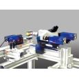
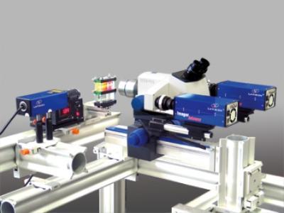
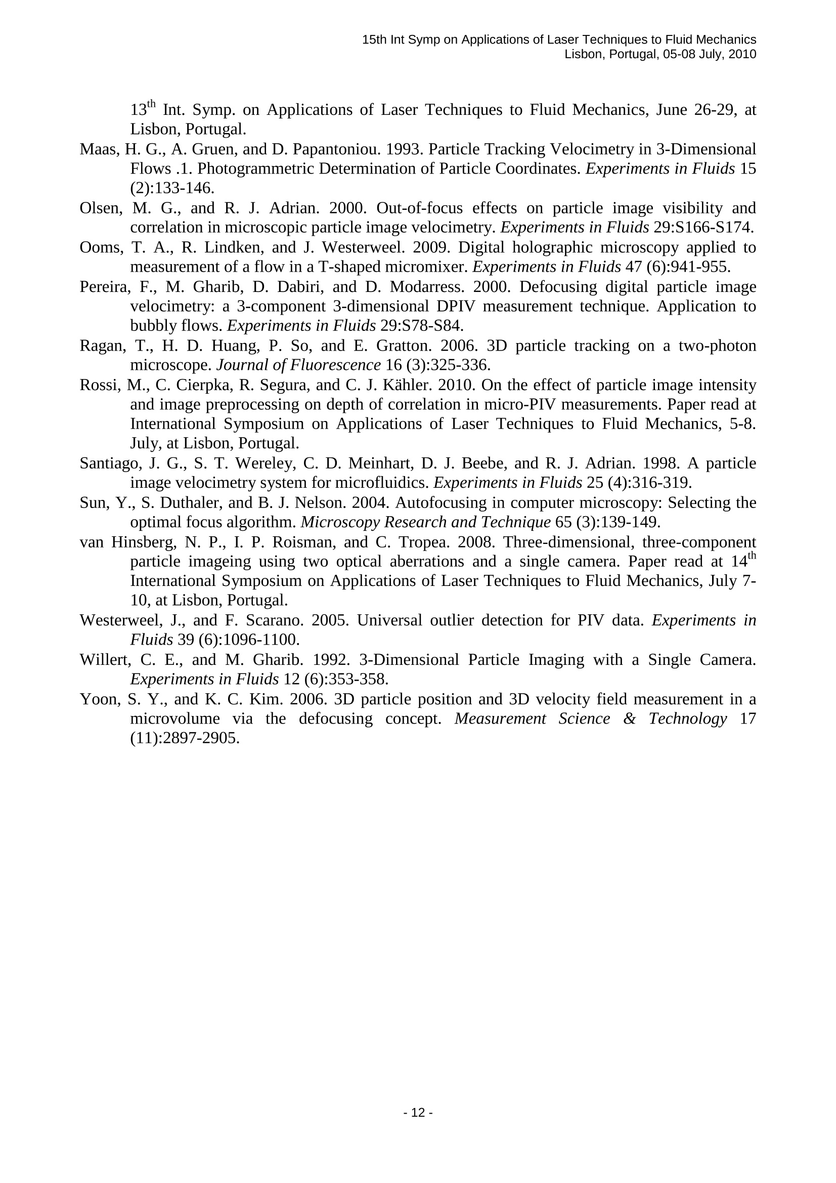
北京欧兰科技发展有限公司为您提供《微流体中速度场,2D3C速度场检测方案(粒子图像测速)》,该方案主要用于其他中速度场,2D3C速度场检测,参考标准--,《微流体中速度场,2D3C速度场检测方案(粒子图像测速)》用到的仪器有显微粒子成像测速系统(Micro PIV)
推荐专场


相关方案
更多
该厂商其他方案
更多