


方案详情
文
The flow generated by heat convection in a long, vertical channel is
studied by means of particle imagery velocimetry techniques, with the help of the
thermal measurements from a previous paper (Gibert et al 2009 Phys. Fluids 21
035109). We analyse the mean velocity profiles and the Reynolds stresses, and
compare the present results with the previous ones obtained in a larger cell and
at a larger Reynolds number.We calculate the horizontal temperature profile and
the related horizontal heat flux. The pertinence of effective turbulent diffusivity
and viscosity is confirmed by the low value of the associated mixing length.
We study the one-point and two-point statistics of both velocity components.
We show how the concept of turbulent viscosity explains the relations between
the local probability density functions (pdf) of fluctuations for temperature,
vertical and horizontal velocity components. Despite the low Reynolds number
values explored, some conclusions can be drawn about the small scale velocity
differences and the related energy cascade.
4 Author
方案详情

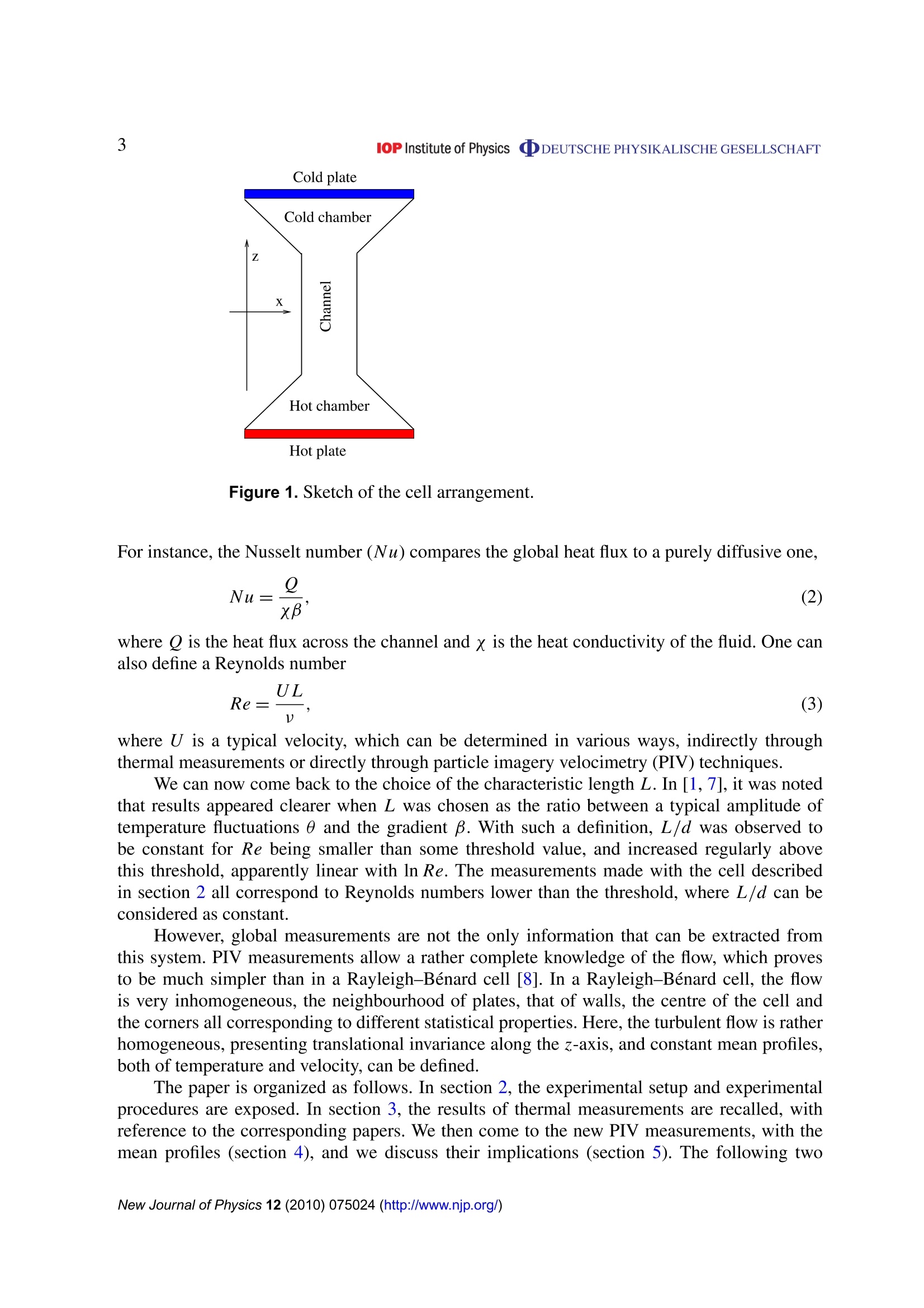
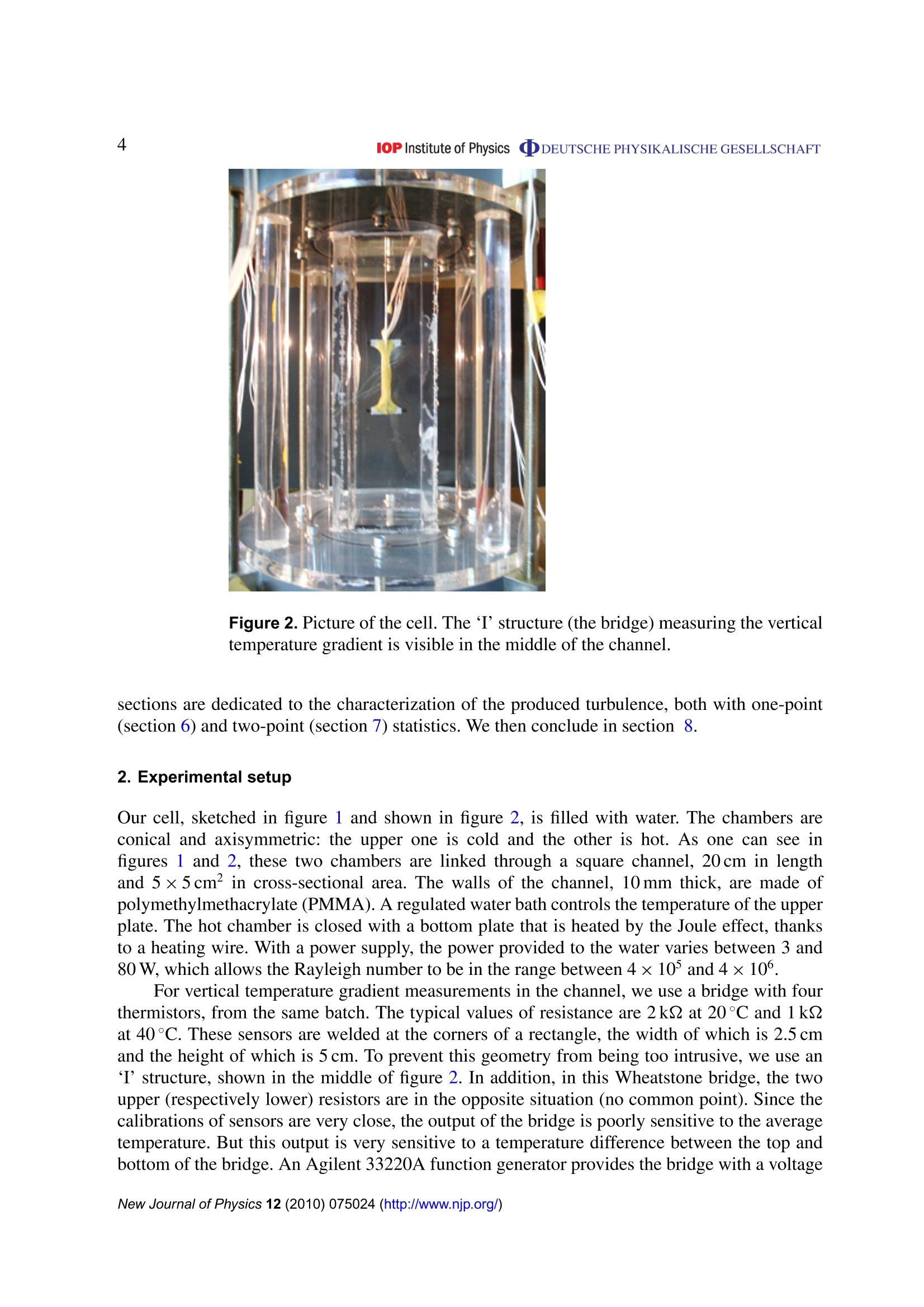
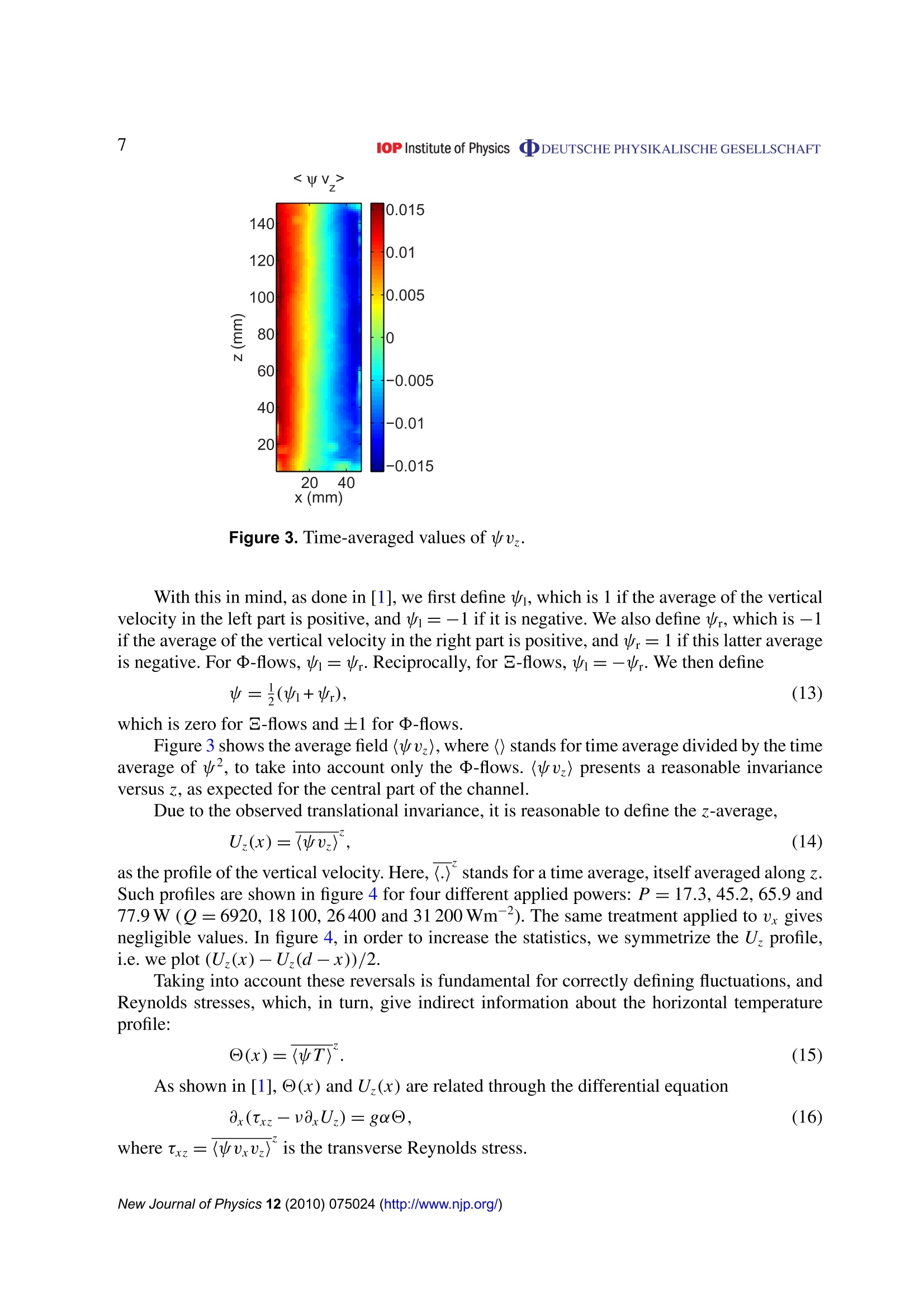
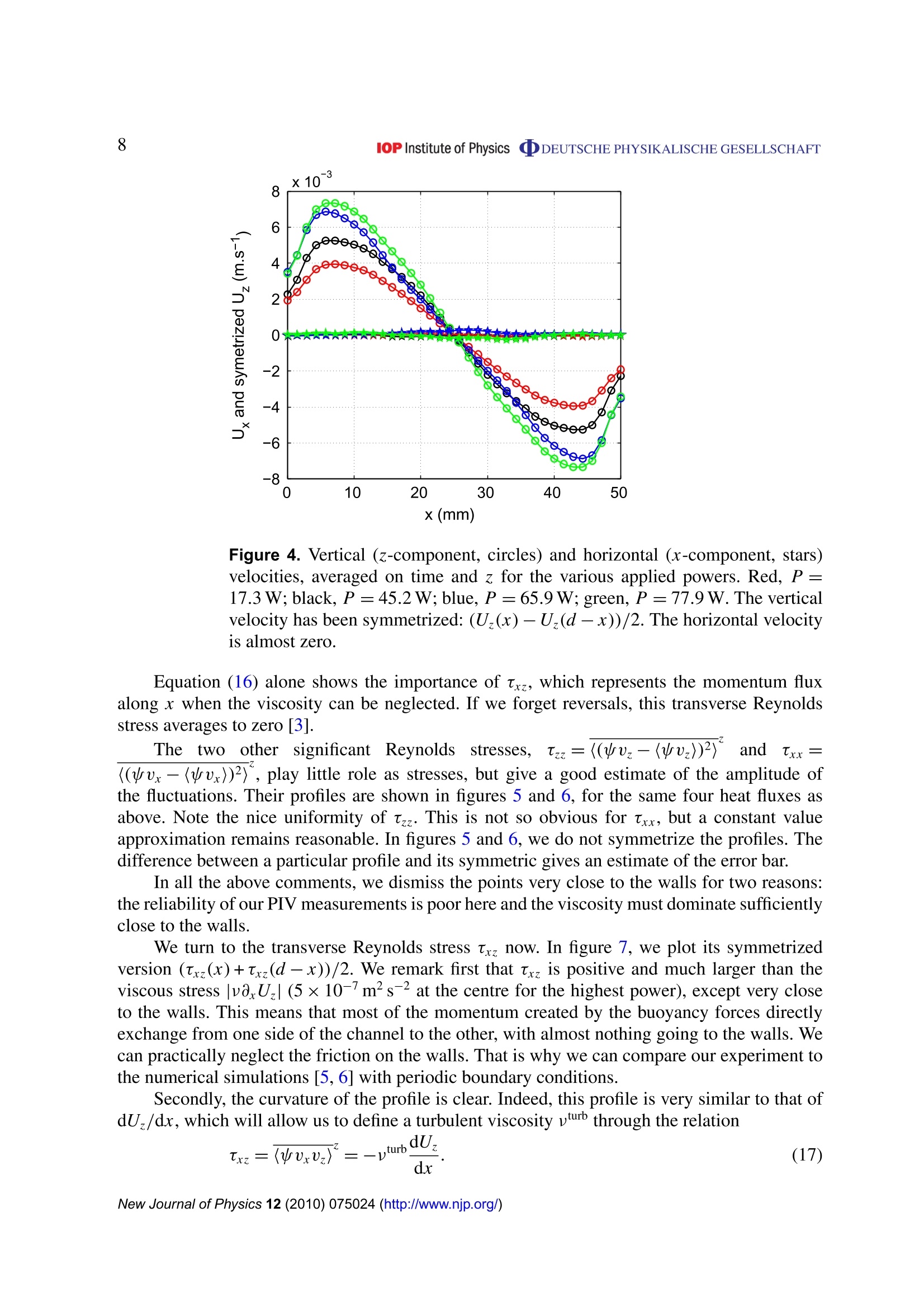
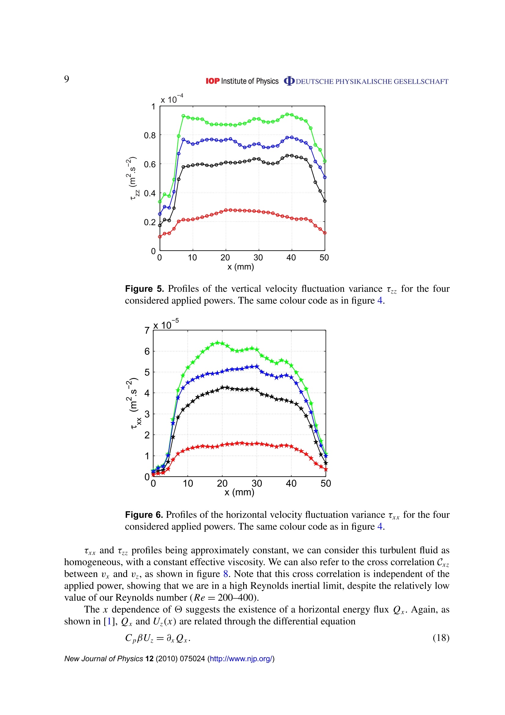
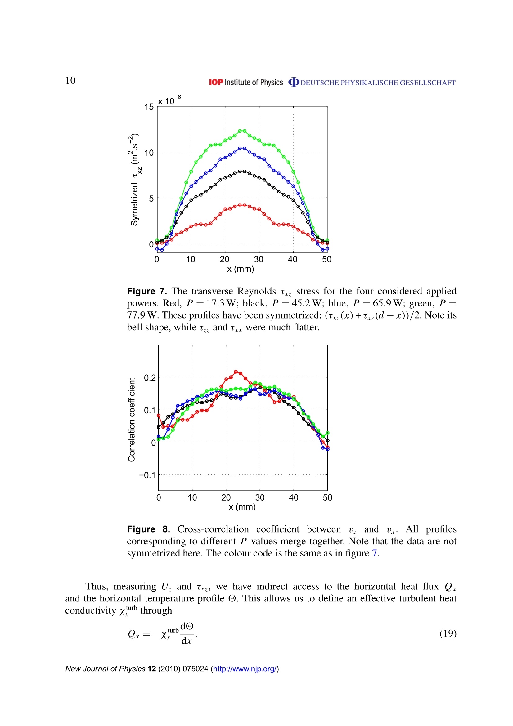
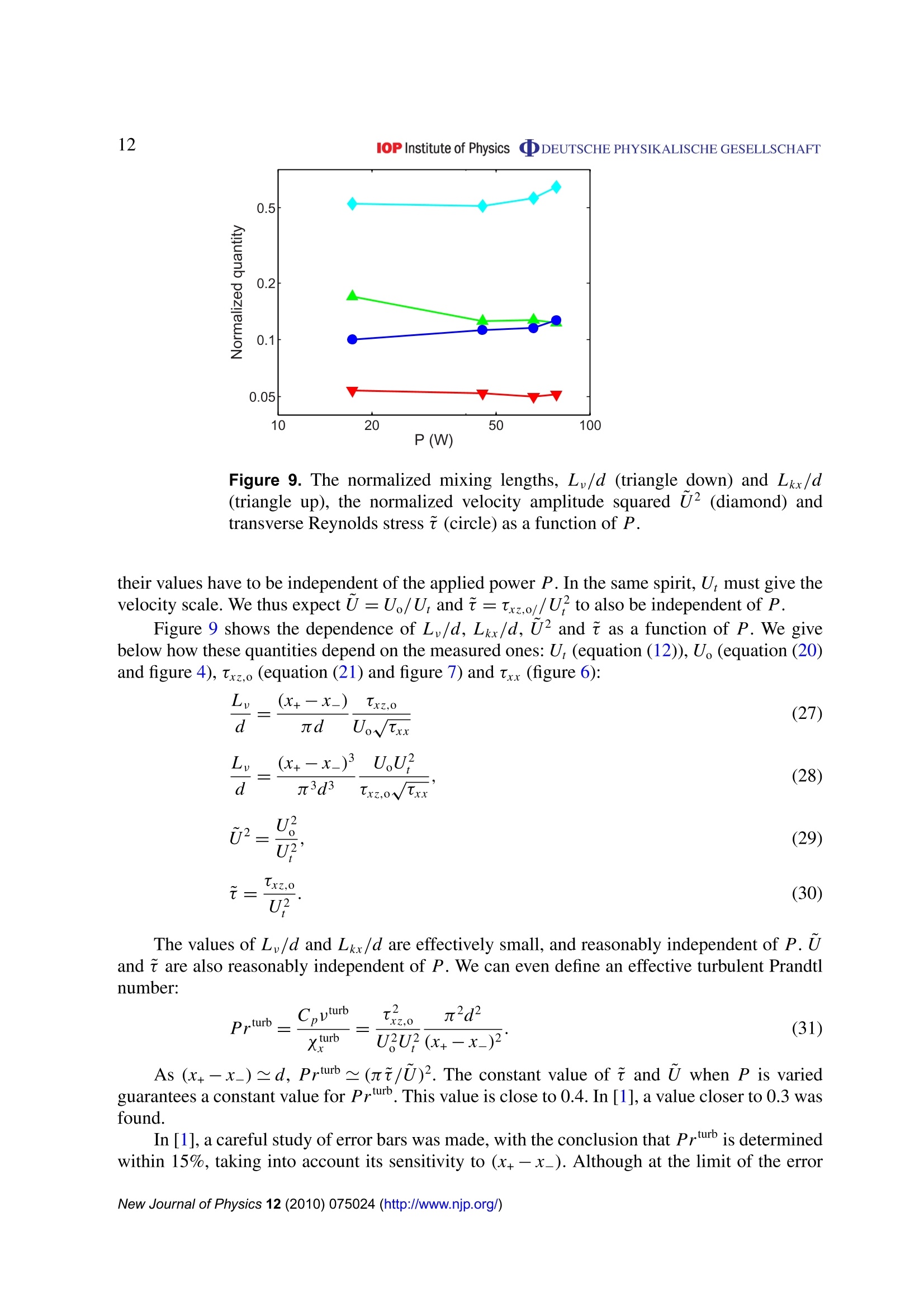
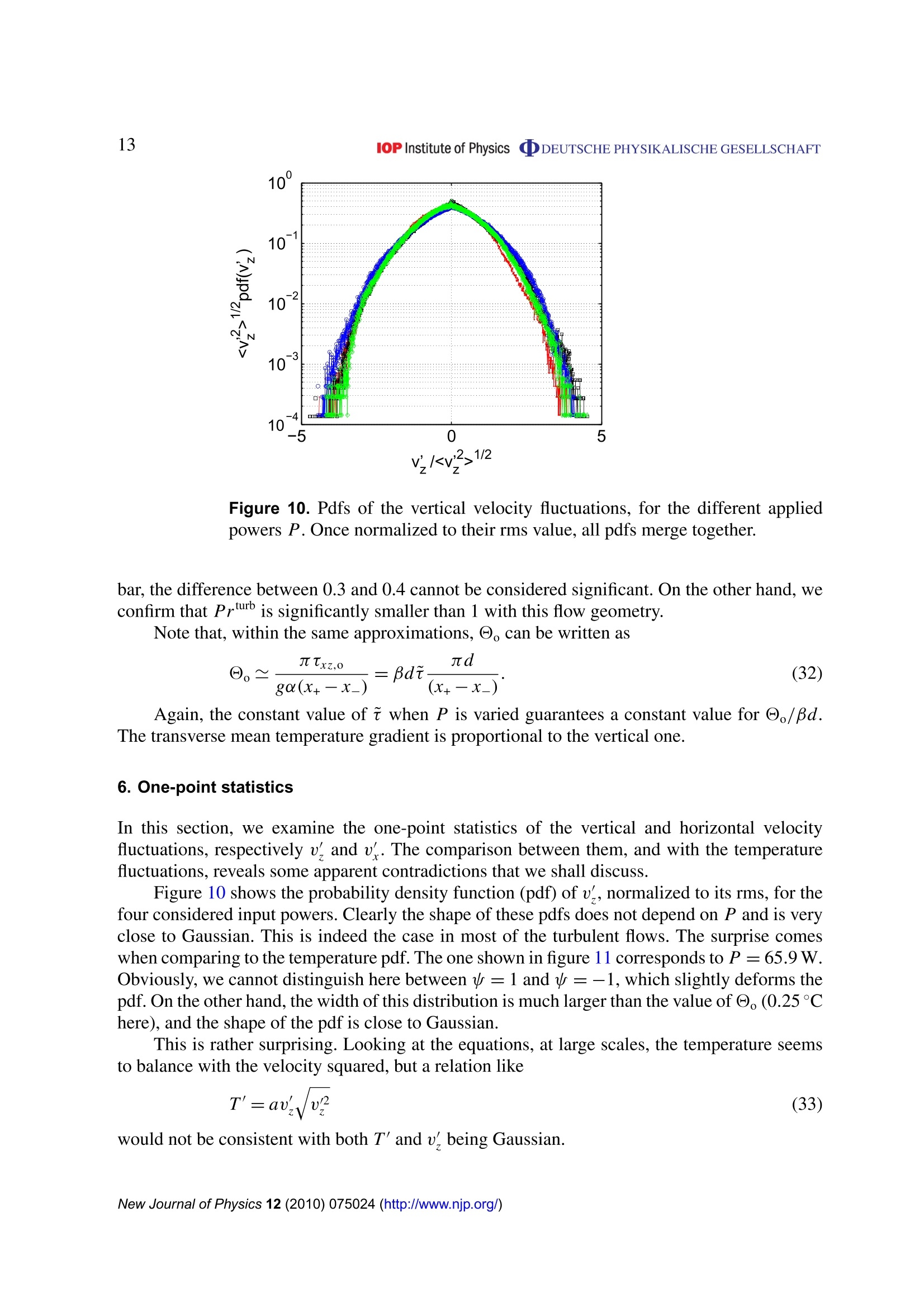
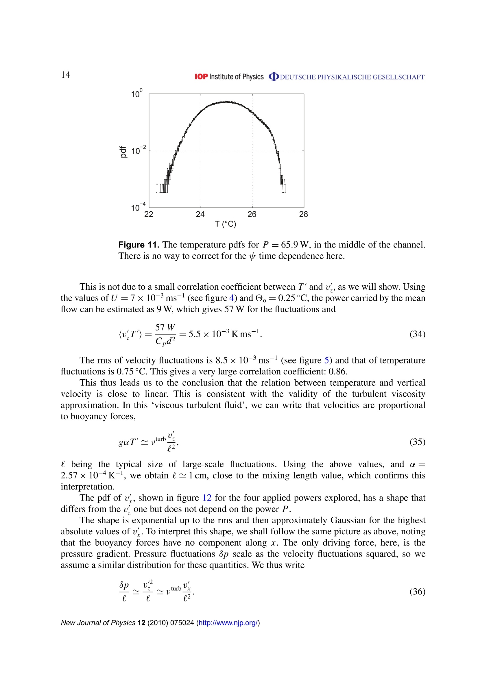
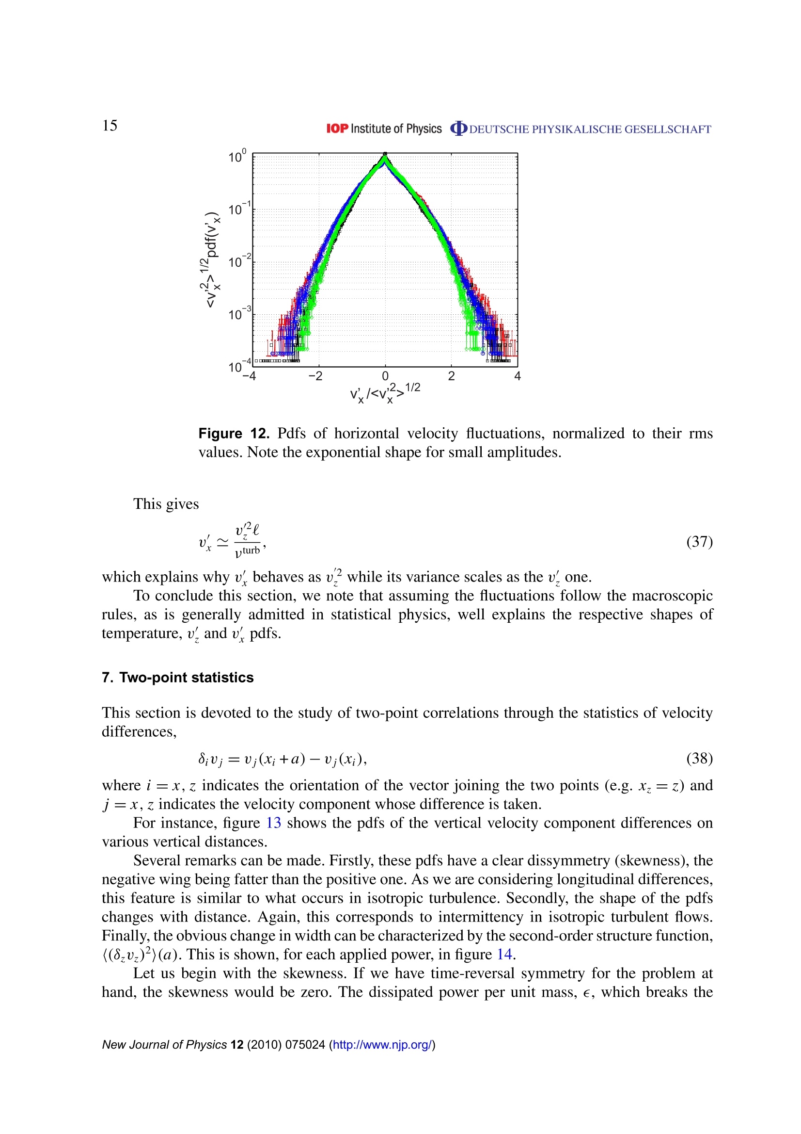
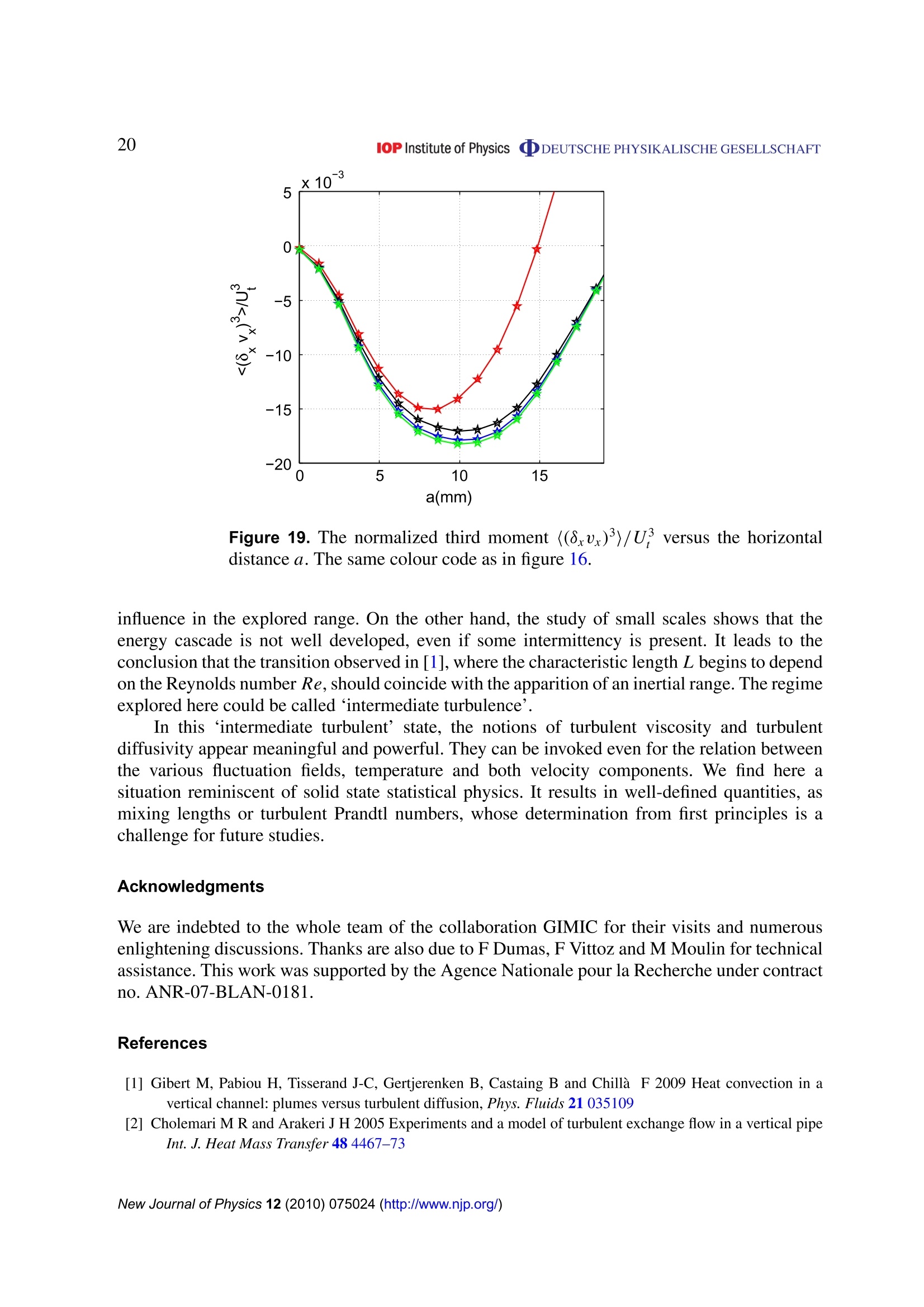
iopscience.iop.org 2IOPInstitute of PhysicsCDDEUTSCHE PHYSIKALISCHE GESELLSCHAFT Home Search Collections Journals AbouttContact usMy lOPscience Convection in a vertical channel This article has been downloaded from IOPscience. Please scroll down to see the full text article.2010 New J. Phys. 12 075024 (http://iopscience.iop.org/1367-2630/12/7/075024) View the table of contents for this issue, or go to the journal homepage for more Download details: |P Address: 202.108.18.194 The article was downloaded on 06/02/2011 at 04:32 Please note that terms and conditions apply. Convection in a vertical channel J-C Tisserand', M Creyssels12, M Gibertl,3, B Castaing andF Chilla1,4 Universite de Lyon, ENS Lyon, UMR 5672 CNRS, 46 Allee d'Italie,69364 Lyon Cedex 7, France"Ecole Centrale Lyon, LMFA CNRS, BP 163, 69131 Ecully Cedex, FranceMPI-DS (LFPN), Gottingen, GermanyE-mail: Francesca.Chilla@ens-lyon.fr New Journal of Physics 12 (2010) 075024 (21pp) Received 11 February 2010 Published 28 July 2010 doi:10.1088/1367-2630/12/7/075024 Abstract. The flow generated by heat convection in a long, vertical channel isstudied by means of particle imagery velocimetry techniques, with the help of thethermal measurements from a previous paper (Gibert et al 2009 Phys. Fluids 21035109). We analyse the mean velocity profiles and the Reynolds stresses, andcompare the present results with the previous ones obtained in a larger cell andat a larger Reynolds number. We calculate the horizontal temperature profile andthe related horizontal heat flux. The pertinence of effective turbulent diffusivityand viscosity is confirmed by the low value of the associated mixing length.We study the one-point and two-point statistics of both velocity components.We show how the concept of turbulent viscosity explains the relations betweenthe local probability density functions (pdf) of fluctuations for temperature,vertical and horizontal velocity components. Despite the low Reynolds numbervalues explored, some conclusions can be drawn about the small scale velocitydifferences and the related energy cascade. ( 4 Author to whom any correspondence should be a ddressed. ) Contents 1. Introduction 2 2. Experimental setup 4 3.]Brief overview of thermal results 5 4.1Mean transverse profiles 6 5.1Mean flow discussion 11 6One-point statistics 1378 Two-point statistics 15 . Conclusions Acknowledgments References 20 1. Introduction Free convection in a long vertical channel is particularly well designed for modelling naturalconvection, such as that occurring in stars, in a planet’s atmosphere or in half-natural situations,such as industrial plants. It allows the study of mixing phenomena in the bulk of the fluid, farfrom scalar injecting boundaries, with a minimum number of control parameters. The first oneis the Prandtl number Pr=v/k, wherev is the kinematic viscosity and k the heat diffusivity.The second control parameter is the Rayleigh number, where g is the gravitational acceleration and a the constant pressure thermal expansioncoefficient. B and L deserve a wider explanation. Let us choose the origin of the temperature T such that its time and space average, onthe whole channel, is zero. (T) is the time-averaged temperature and β=-d(T)/dz is thetemperature gradient that drives the flow. If the thermal expansion coefficient α >0, which isthe general case, convection occurs if the hot fluid is below the cold one (B>0). L is a characteristic length of the flow. The natural choice is d, the width of the channel.In a recent paper [1], thermal measurements yield another choice for L. We shall come back tothis point later. For experimental realizations, the considered channel connects two chambers, the hot oneat the bottom and the cold one at the top. The sketch of such an experiment is shown in figure 1. Note that salted water has been used for a similar study. For instance, the authors of [2]-[4]looked at the free convection in a vertical tube connecting two chambers with different saltconcentrations. They studied a flux of salt instead of a flux of heat, and the salt diffusioncoefficient (respectively the Schmidt number Sc) takes the place of k (respectively Pr). Somenumerical simulations [5, 6] also correspond well to this situation, using periodic boundaryconditions. As in the Rayleigh-Benard case (the other great paradigm in thermal convection), the stateof the system can be characterized by its global response to the above applied parameters. Figure 1. Sketch of the cell arrangement. For instance, the Nusselt number (Nu) compares the global heat flux to a purely diffusive one, where is the heat flux across the channel and x is the heat conductivity of the fluid. One canalso define a Reynolds number where U is a typical velocity, which can be determined in various ways, indirectly throughthermal measurements or directly through particle imagery velocimetry (PIV) techniques. We can now come back to the choice of the characteristic length L. In [1, 7], it was notedthat results appeared clearer when L was chosen as the ratio between a typical amplitude oftemperature fluctuations 0 and the gradient B. With such a definition, L/d was observed tobe constant for Re being smaller than some threshold value, and increased regularly abovethis threshold, apparently linear with ln Re. The measurements made with the cell describedin section 2 all correspond to Reynolds numbers lower than the threshold, where L/d can beconsidered as constant. However, global measurements are not the only information that can be extracted fromthis system. PIV measurements allow a rather complete knowledge of the flow, which provesto be much simpler than in a Rayleigh-Benard cell [8]. In a Rayleigh-Benard cell, the flowis very inhomogeneous, the neighbourhood of plates, that of walls, the centre of the cell andthe corners all corresponding to different statistical properties. Here, the turbulent flow is ratherhomogeneous, presenting translational invariance along the z-axis, and constant mean profiles,both of temperature and velocity, can be defined. The paper is organized as follows. In section 2, the experimental setup and experimentalprocedures are exposed. In section 3, the results of thermal measurements are recalled, withreference to the corresponding papers. We then come to the new PIV measurements, with themean profiles (section 4), and we discuss their implications (section 5). The following two Figure 2. Picture of the cell. The‘I’structure (the bridge) measuring the verticaltemperaturegradient is visible in the middle of the channel. sections are dedicated to the characterization of the produced turbulence, both with one-point(section 6) and two-point (section 7) statistics. We then conclude in section 8. 2. Experimental setup Our cell, sketched in figure 1 and shown in figure 2, is filled with water. The chambers areconical and axisymmetric: the upper one is cold and the other is hot. As one can see infigures 1 and 2, these two chambers are linked through a square channel, 20 cm in lengthand 5×5 cm in cross-sectional area. The walls of the channel, 10mm thick, are made ofpolymethylmethacrylate (PMMA). A regulated water bath controls the temperature of the upperplate. The hot chamber is closed with a bottom plate that is heated by the Joule effect, thanksto a heating wire. With a power supply, the power provided to the water varies between 3 and80 W, which allows the Rayleigh number to be in the range between 4 ×10and 4×10°. For vertical temperature gradient measurements in the channel, we use a bridge with fourthermistors, from the same batch. The typical values of resistance are 2k9 at 20°C and 1kat 40C. These sensors are welded at the corners of a rectangle,the width of which is 2.5 cmand the height of which is 5 cm. To prevent this geometry from being too intrusive, we use anT’structure, shown in the middle of figure 2. In addition, in this Wheatstone bridge, the twoupper (respectively lower) resistors are in the opposite situation (no common point). Since thecalibrations of sensors are very close, the output of the bridge is poorly sensitive to the averagetemperature. But this output is very sensitive to a temperature difference between the top andbottom of the bridge. An Agilent 33220A function generator provides the bridge with a voltage with a range of 0.1 V and with a frequency of 34 Hz. We measure the output of the bridge witha differential lock-in amplifier (Stanford Research SR8303DSP). To carry out PIV, we use a one watt green continuous laser (Melles Griot). In a first step, weseed water with hollow glass particles (Sphericel 110P8, LaVision GmbH), 10 um in averagediameter. A laser sheet (DPSS-Laser System, 532 nm, Melles Griot) is created, thanks to acylindrical lens. We record images of the channel with the Imager Pro Lavision camera. All ourPIV measurements are made at a frequency of 25 Hz and the recording and batch processing aredone with Davis Lavision’s software. The images are grouped in blocks of 20 (0.8 s for the block). The blocks are separated by2 min, much larger than the correlation time of velocity (see [1]). A record consists of 160 blocks(which corresponds to 5 h and 20 min). All the records are made at an average temperature of25°℃(Pr=6), close to the room temperature, to minimize eventual heat leaks. 3. Brief overview of thermal results The output of the bridge gives us all the global information on our system. In the absenceof convection (no heat flux), it presents no visible fluctuations, which allows us to preciselymeasure the zero of our bridge. It also allows us to finely check the eventual heat leaks onour hot chamber, which enhance our precision on the heat flux Q. The average value of theoutput gives us the temperature gradient B. We checked that its value is reasonably constantwhen translating the I’structure along the axis of the cell [1]. Assuming a short correlationlength for the temperature field (we verified this hypothesis), the rms value of the output givesan amplitude 0 for the temperature fluctuations. With the ratio between 0 and β, we can definean ‘intrinsic’length Furthermore, the cut-off frequency of the bridge output power spectrum givescharacteristic time t. We verified that L/t is systematically close to the root mean square (rms)value of the velocity. Thus, the only measure of the bridge output gives us the gradient β, thelength L and thus the Rayleigh number Ra and the Reynolds number if we define it by In[1], it has been shown that all the data, whether of the present cell or of another one withd twice larger (called“the previous cell'hereafter), at various Prandtl numbers Pr,agree withthe following laws: It is worth mentioning that, with our choice for L,the close similitude between Nu andRePr has a simple interpretation. The heat flux O can be written as where C, is the heat capacity per unit volume (x=Cpk). ((.))means averaging both on timeand the width of the channel. Then, the Nusselt number Nu= New Journal of Physics 12 (2010) 075024 (http://www.njp.org/) with where 8T=T-((T)) is the difference between the instantaneous temperature T and itsaverage. CuT is the correlation coefficient between u and T. Considering, as we assume, that O, used in the definition of L (equation (4)), is proportionalto√((8T2)) and U to√((v)), we can write If Cr is constant, the choice we made for L ensures similar behaviour between Nu and RePr. In a previous study [1], we used a cell (the previous cell’) with the same channel length ashere (20 cm) and a width twice as large. Despite this difference in aspect ratio, the Nu versusRa and Re versus Ra were in agreement with equation (6). As noted in [1], the same agreementis found with the salt water experiments [2, 3] and the numerical simulations [5, 6]. In the following, all measurements concern velocities, with no direct measure of p and thusof L. The only thermal information is the heat power input to the hot plate. It is thus useful totranslate p in terms of a velocity squared, which is the square of the free fall velocity, under the buoyancy acceleration, on a length d.Taking into account that, in the regime we explore, L0.8d, the relation Nu=1.6√RaPrgives which we take as the definition of our reference velocity U,. 4. Mean transverse profiles In [1], a PIV study was analysed, for two different input powers, in the ‘previous cell’. In thissection, we report a similar study, systematically performed for four different input powers, inour present cell. The goal is multiple. First, we want to check the expected scalings, both withspatial dimensions and the input power. We also want to check the pertinence of the turbulentviscosity approximation, in the present situation, where the Reynolds number is significantlylower than in [1]. Indeed, we shall see in the next section the importance of this conceptof turbulent viscosity for interpreting the relation between temperature and vertical velocityfluctuations. To correctly analyse the flow through PIV techniques, it is very important to take intoaccount one of its characteristics: it often separates into two columns, one ascending and theother descending. In most of the pictures, the flow is globally ascending in the left-hand part and descendingin the right one, or the opposite. These flows we call D-flows. Some of the pictures show aflow globally ascending in both parts (remember that we record only a sheet of the flow) ordescending. We call this kind of flow E-flows. D-flows have a typical mixing layer structure.In order to discuss them, first we have to extract the average profile of the velocity field. Figure 3. Time-averaged values of wu. With this in mind, as done in [1], we first define vi, which is 1 if the average of the verticalvelocity in the left part is positive, and vi=-1 if it is negative. We also define vr, which is -1if the average of the vertical velocity in theright part is positive, and vr=1 if this latter averageis negative. For D-flows,vi=vr.Reciprocally, for E-flows,vi=-Vr. We then define which is zero for E-flows and ±1 for D-flows. Figure 3 shows the average field (wuz), where () stands for time average divided by the timeaverage of 2, to take into account only the D-flows. (vu) presents a reasonable invarianceversus z, as expected for the central part of the channel. Due to the observed translational invariance, it is reasonable to define the z-average, as the profile of the vertical velocity. Here, (.) stands for a time average, itself averaged along z.Such profiles are shown in figure 4 for four different applied powers: P=17.3, 45.2, 65.9 and77.9 W (Q=6920, 18100, 26 400 and 31 200 Wm-). The same treatment applied to ux givesnegligible values. In figure 4, in order to increase the statistics, we symmetrize the Uz profile,i.e. we plot (Uz(x)-U(d-x))/2. Taking into account these reversals is fundamental for correctly defining fluctuations, andReynolds stresses, which, in turn, give indirect information about the horizontal temperatureprofile: As shown in [1],Q(x) and U (x) are related through the differential equation 0x(txz-voxUz)=go@, (16) where txz =(vuxvz) is the transverse Reynolds stress. Figure 4. Vertical (z-component, circles) and horizontal (x-component, stars)velocities, averaged on time and z for the various applied powers. Red, P=17.3 W; black, P =45.2 W; blue, P=65.9 W; green, P = 77.9 W. The verticalvelocity has been symmetrized: (Uz(x)-U(d-x))/2. The horizontal velocityis almost zero. Equation (16) alone shows the importance of txz, which represents the momentum fluxalong x when the viscosity can be neglected. If we forget reversals, this transverse Reynoldsstress averages to zero [3]. The two other significant Reynoldsstresses.t=((wu-(wu))2) andtxx=((vux-(vux))2), play little role as stresses, but give a good estimate of the amplitude ofthe fluctuations. Their profiles are shown in figures 5 and 6, for the same four heat fluxes asabove. Note the nice uniformity of tzz. This is not so obvious for txx, but a constant valueapproximation remains reasonable. In figures 5 and 6, we do not symmetrize the profiles. Thedifference between a particular profile and its symmetric gives an estimate of the error bar. In all the above comments, we dismiss the points very close to the walls for two reasons:the reliability of our PIV measurements is poor here and the viscosity must dominate sufficientlyclose to the walls. We turn to the transverse Reynolds stress txz now. In figure 7, we plot its symmetrizedversion (txz(x)+txz(d-x))/2. We remark first that tz is positive and much larger than theviscous stress |voUzl (5×10⁻⁷m’s-2 at the centre for the highest power), except very closeto the walls. This means that most of the momentum created by the buoyancy forces directlyexchange from one side of the channel to the other, with almost nothing going to the walls. Wecan practically neglect the friction on the walls. That is why we can compare our experiment tothe numerical simulations [5, 6] with periodic boundary conditions. Secondly, the curvature of the profile is clear. Indeed, this profile is very similar to that ofdU,/dx, which will allow us to define a turbulent viscosity pturb through the relation New Journal of Physics 12 (2010) 075024 (http://www.njp.org/) Figure 5. Profiles of the vertical velocity fluctuation variance tz for the fourconsidered applied powers. The same colour code as in figure 4. Figure 6. Profiles of the horizontal velocity fluctuation variance txx for the fourconsidered applied powers. The same colour code as in figure 4. txx and tzz profiles being approximately constant, we can consider this turbulent fluid ashomogeneous, with a constant effective viscosity. We can also refer to the cross correlation Cxzbetween Ux and uz, as shown in figure 8. Note that this cross correlation is independent of theapplied power, showing that we are in a high Reynolds inertial limit, despite the relatively lowvalue of our Reynolds number (Re=200-400). The x dependence of @ suggests the existence of a horizontal energy flux Ox. Again, asshown in [1], Ox and U (x) are related through the differential equation C,BUz=0.0x. (18) Figure 7. The transverse Reynolds txz stress for the four considered appliedpowers. Red, P=17.3 W; black, P =45.2 W; blue, P=65.9 W; green, P=77.9 W. These profiles have been symmetrized: (txz(x)+txz(d-x))/2. Note itsbell shape, while t and txx were much flatter. Figure 8. Cross-correlation coefficient betweenn Uu zand vtx. All profilescorresponding to different P values merge together. Note that the data are notsymmetrized here. The colour code is the same as in figure 7. Thus, measuring Uz and txz, we have indirect access to the horizontal heat flux Oxand the horizontal temperature profile @. This allows us to define an effective turbulent heatconductivity x turb through However, the noise on averaged quantities forbids calculating derivatives as we have inequations (17)-(19). That is why we smooth the obtained profiles through a simplified model. We model the major central part of the flow, setting aside two regions x
确定
还剩20页未读,是否继续阅读?

产品配置单

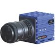
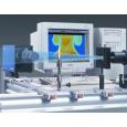
北京欧兰科技发展有限公司为您提供《气流中垂直通道的对流研究检测方案(粒子图像测速)》,该方案主要用于其他中垂直通道的对流研究检测,参考标准--,《气流中垂直通道的对流研究检测方案(粒子图像测速)》用到的仪器有德国LaVision PIV/PLIF粒子成像测速场仪、Imager sCMOS PIV相机、PLIF平面激光诱导荧光火焰燃烧检测系统
推荐专场


相关方案
更多
该厂商其他方案
更多