


方案详情
文
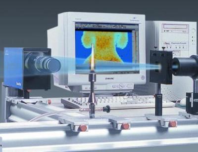
采用LaVision的HS500型CMOS相机和DaVis软件平台以及Nd:YAG激光器,搭建了一套平面激光诱导荧光和粒子成像测速PIV测量平台。利用这一平台对在惯性主导区域下落液体薄膜上的孤立波进行了测量和研究。
方案详情

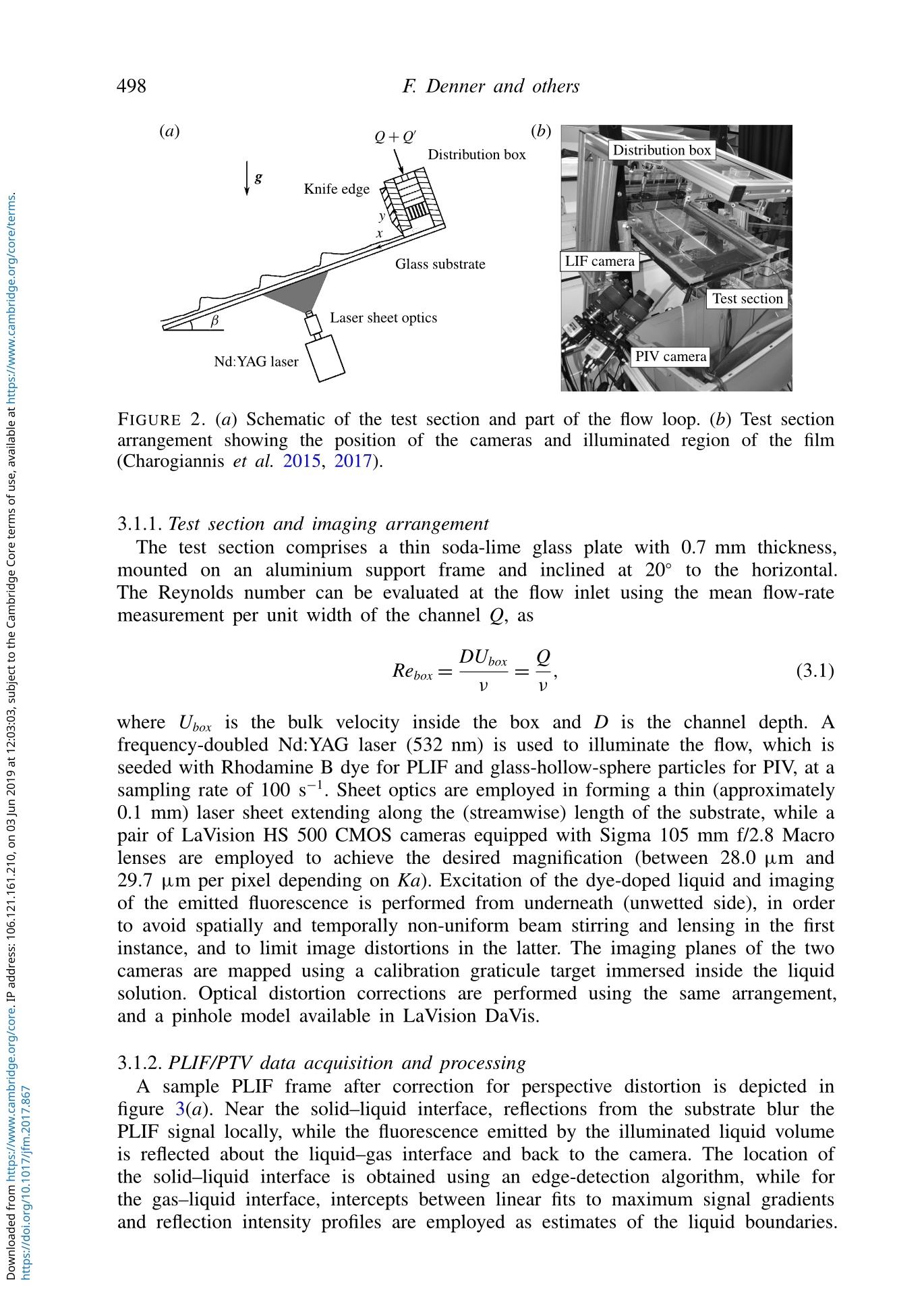
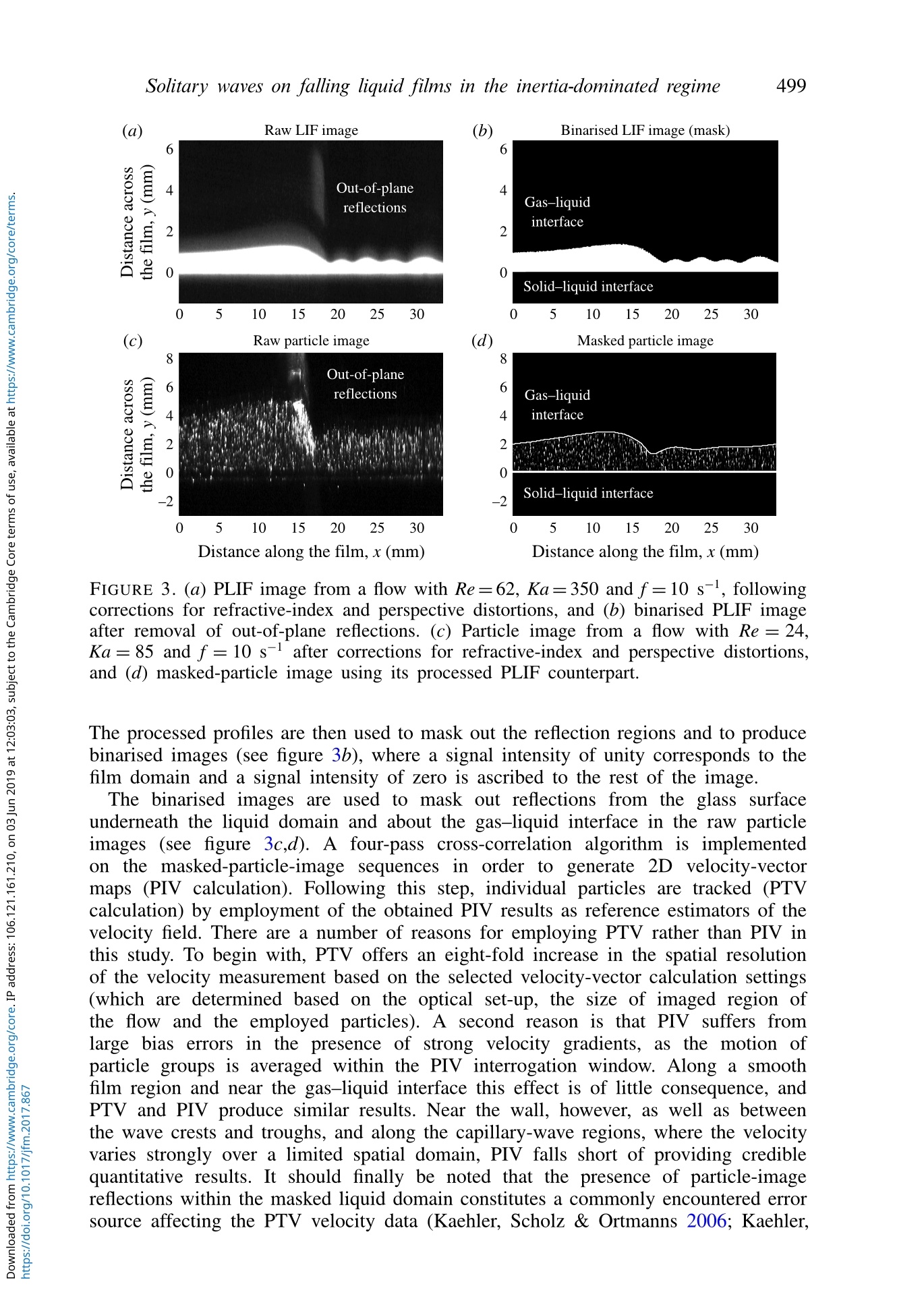
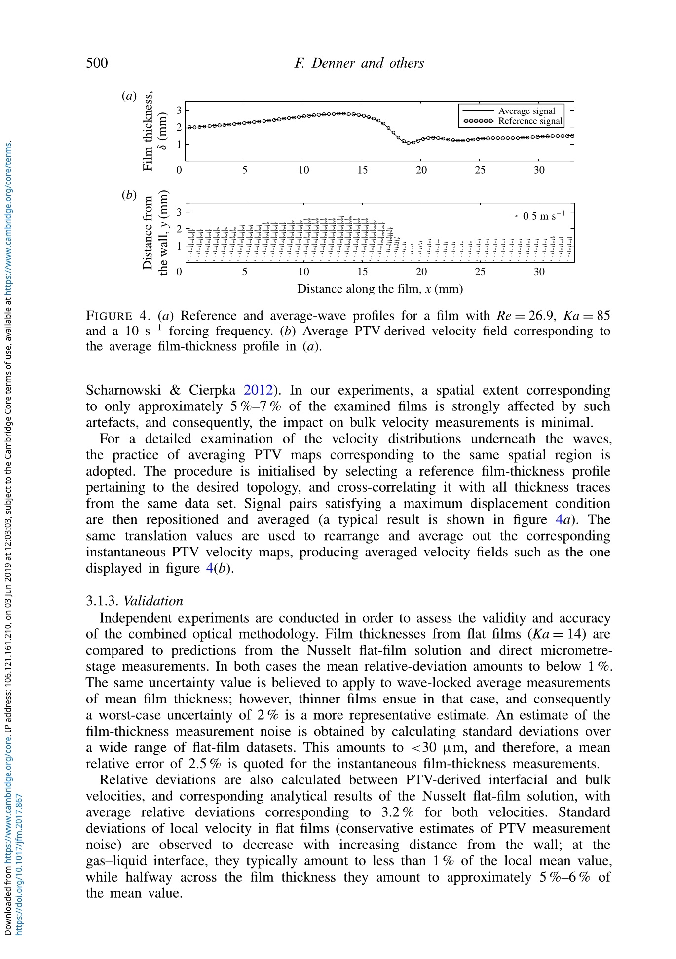
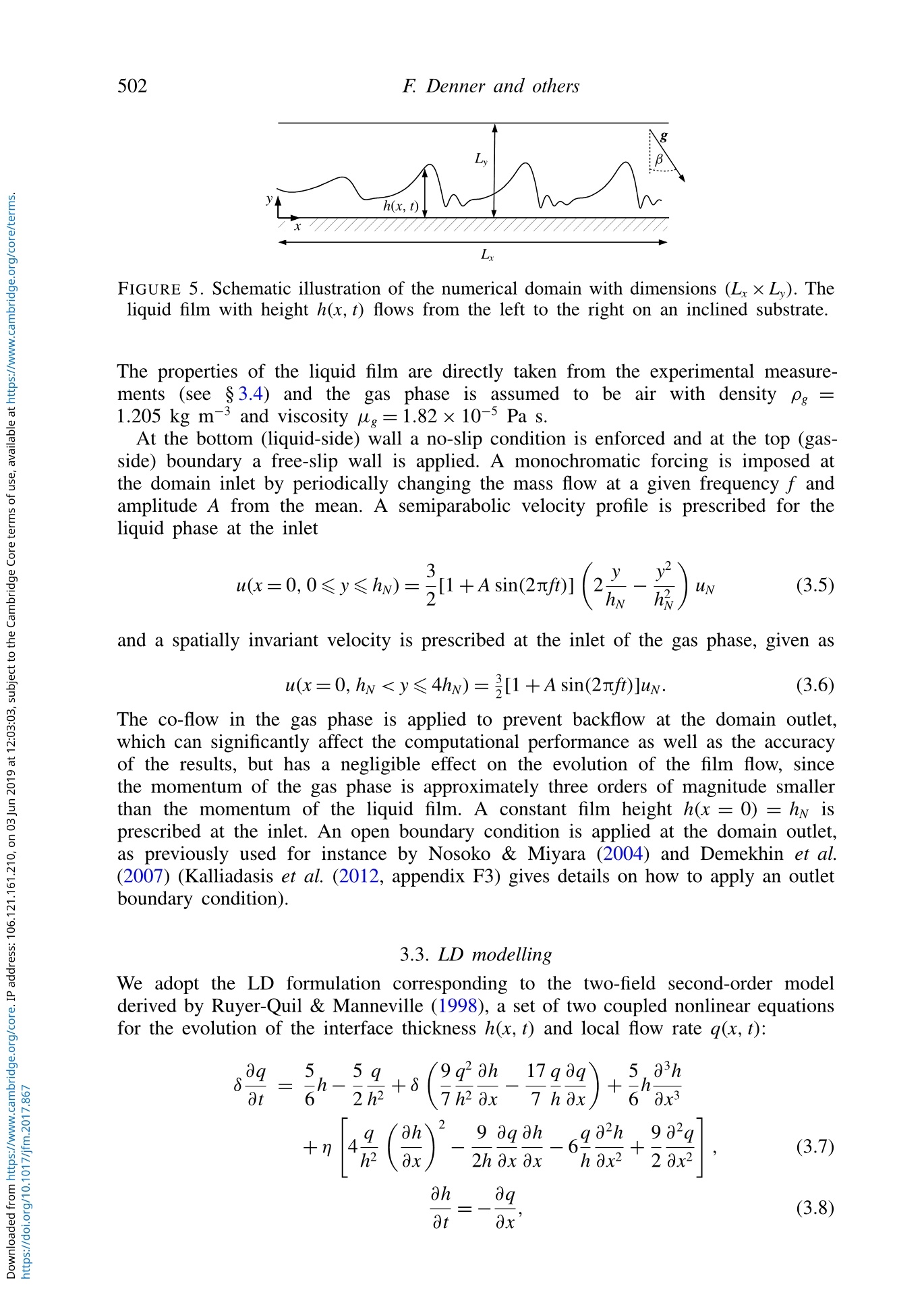
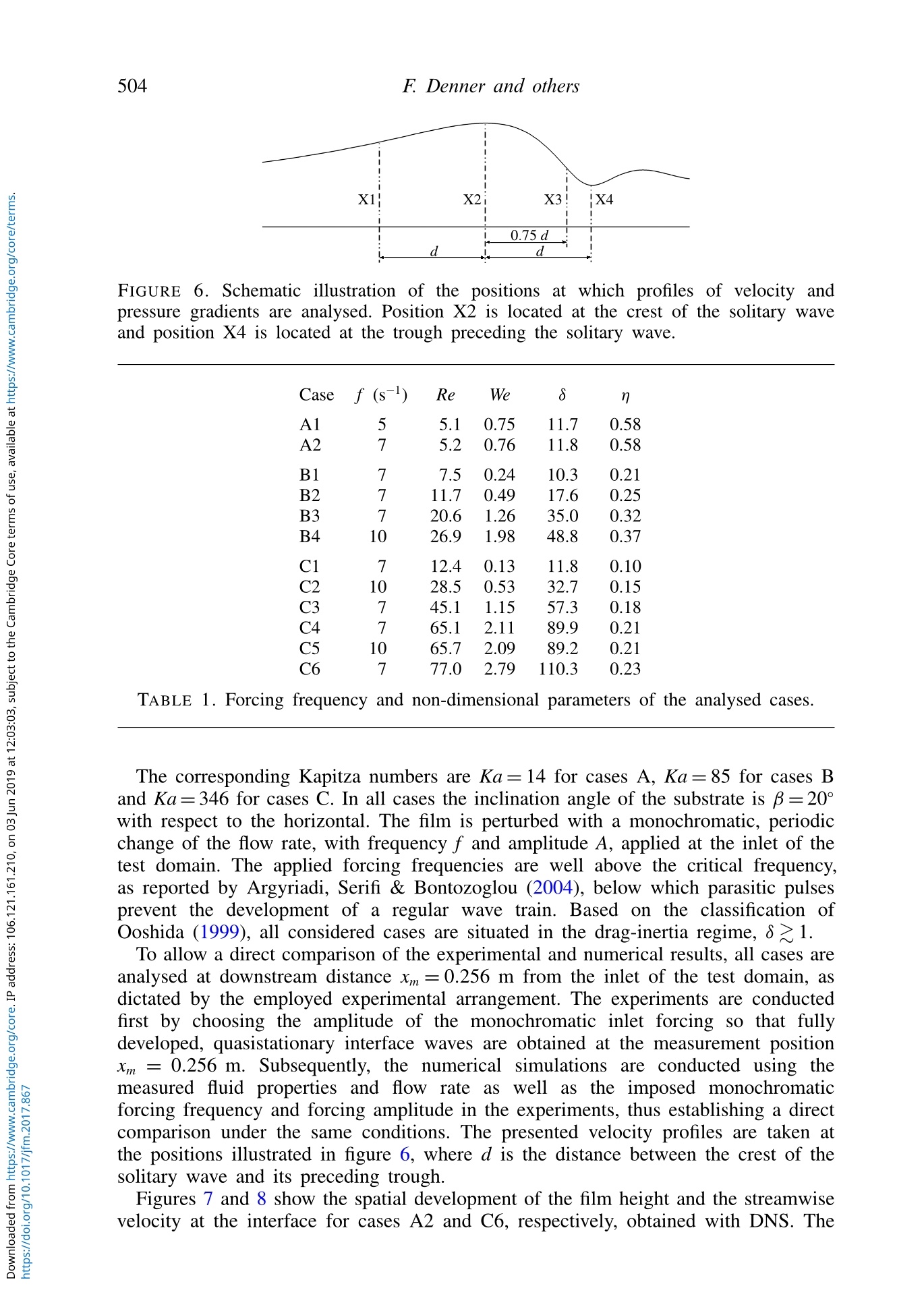
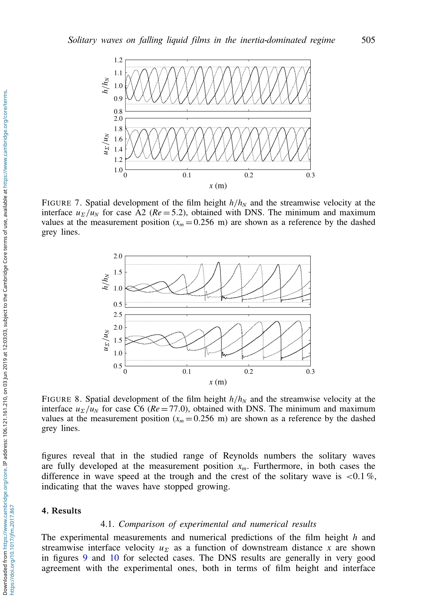
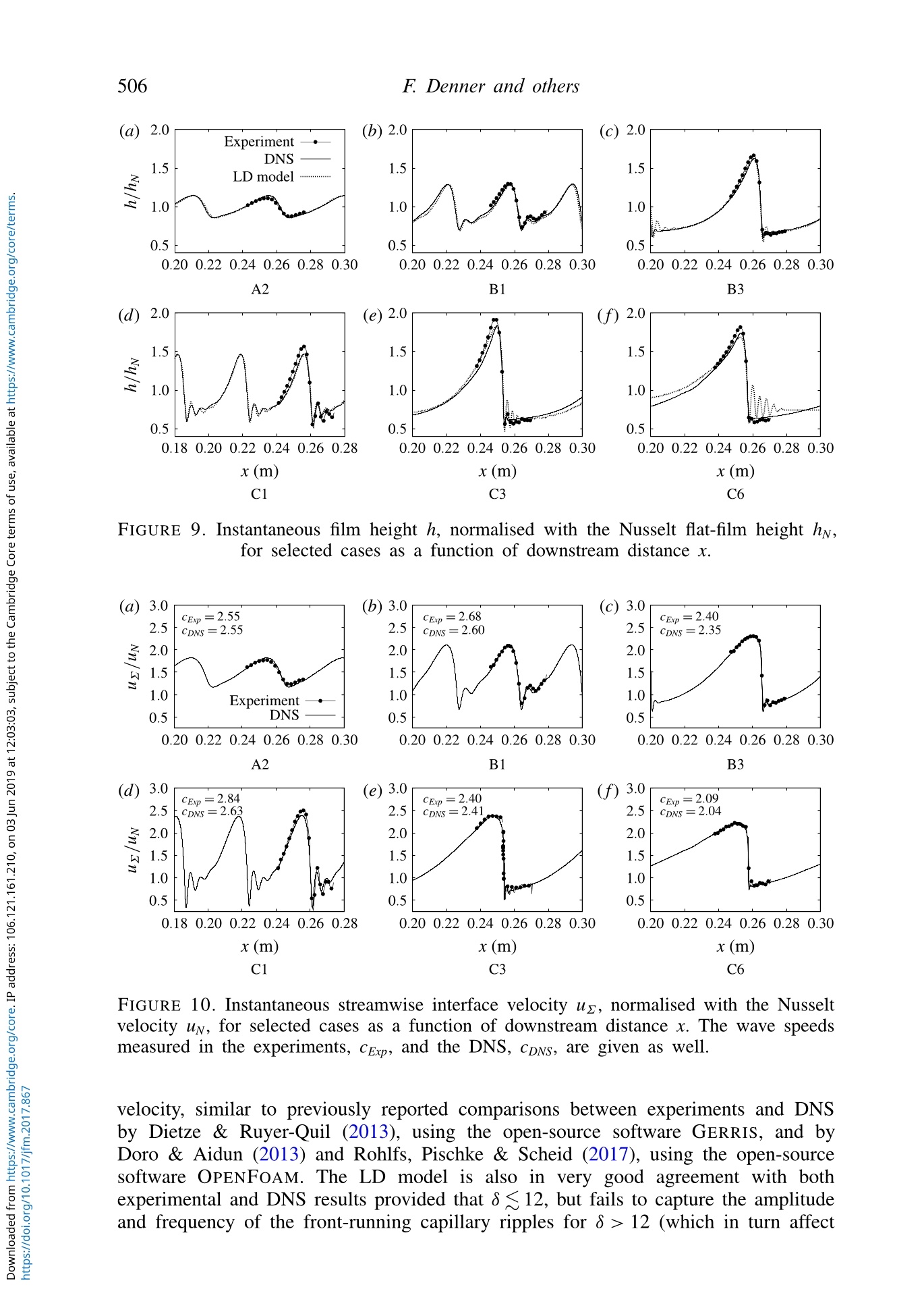
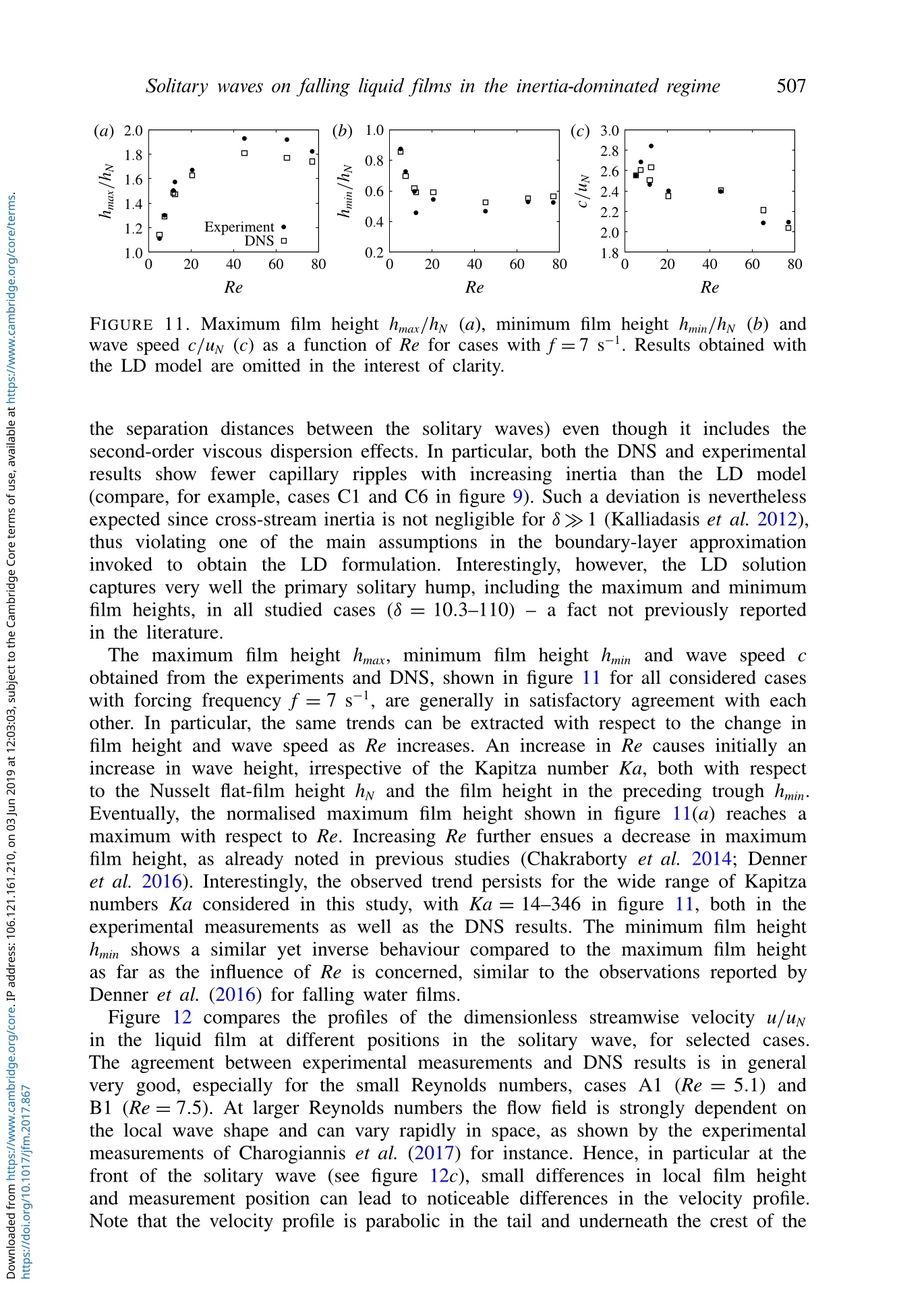
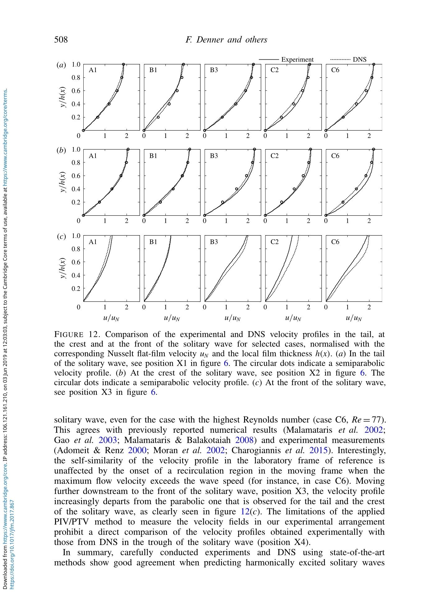
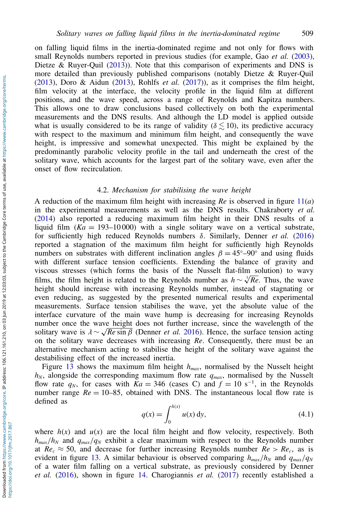
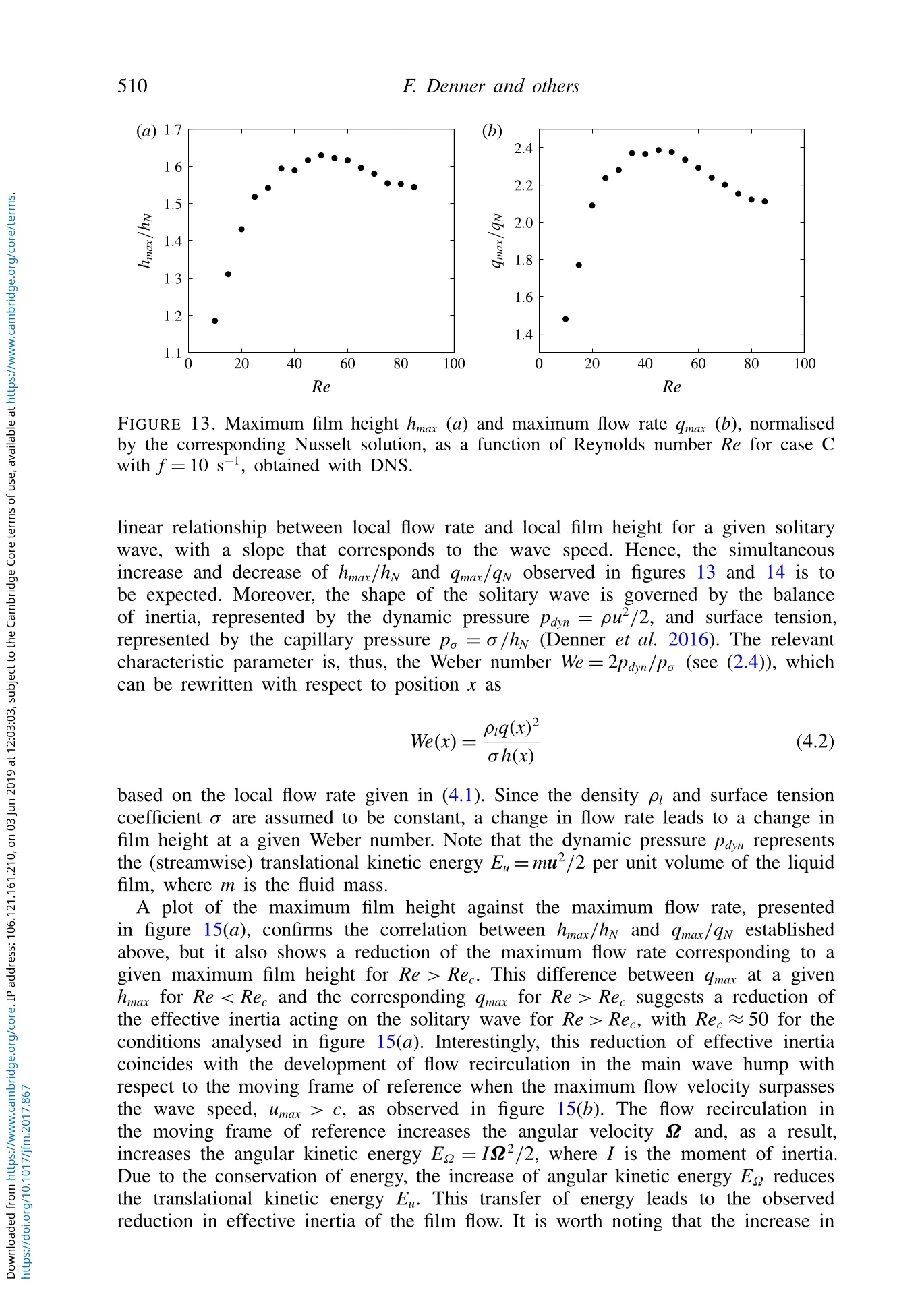
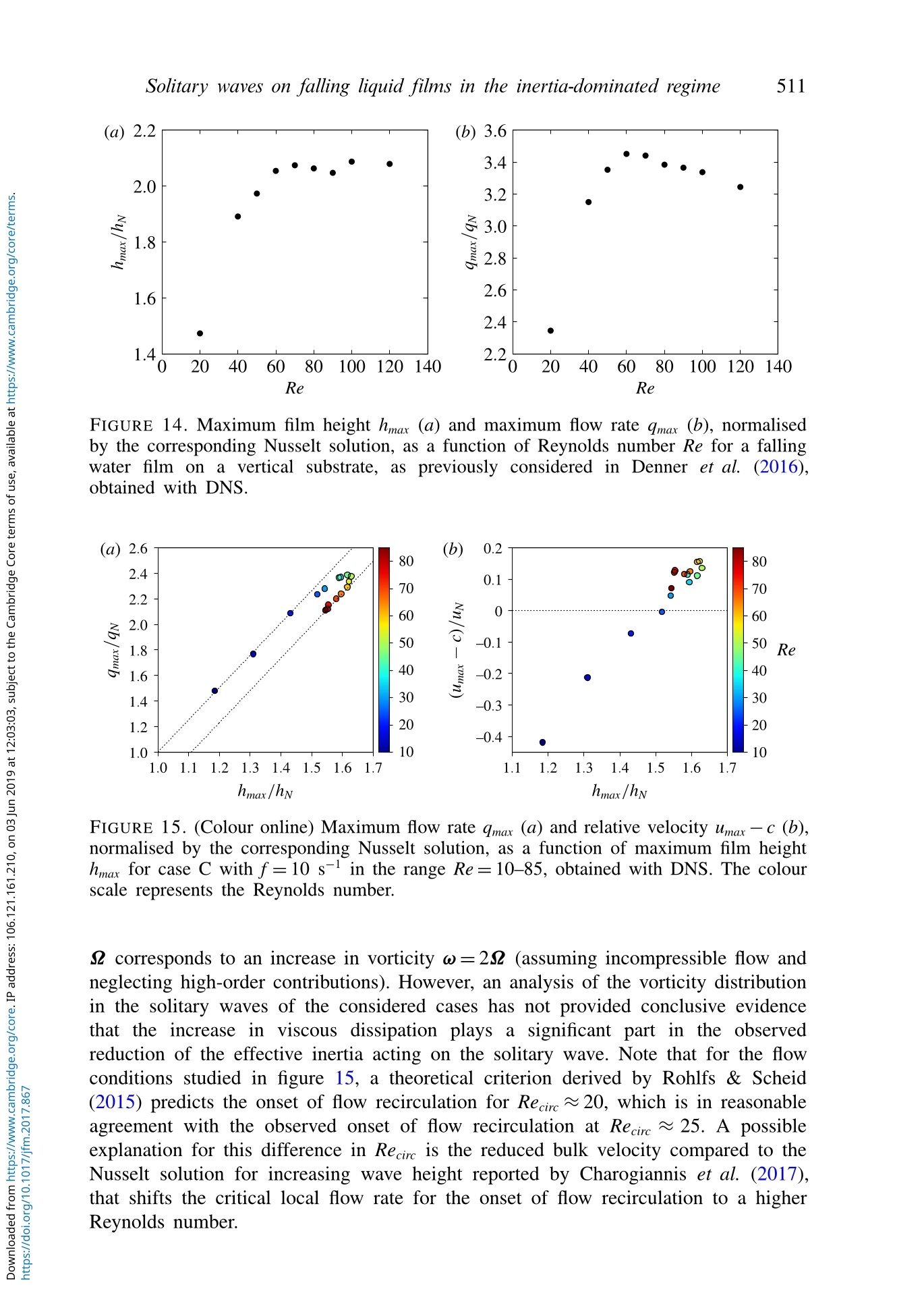
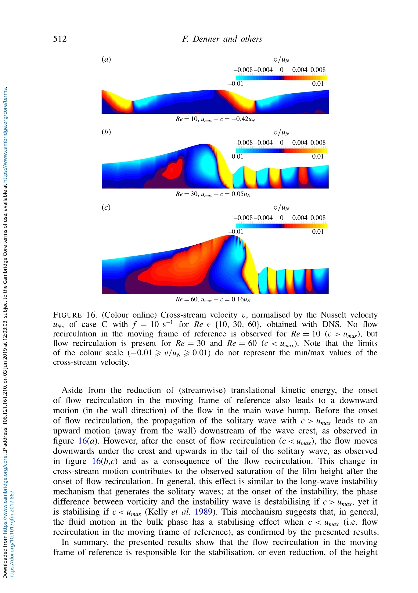
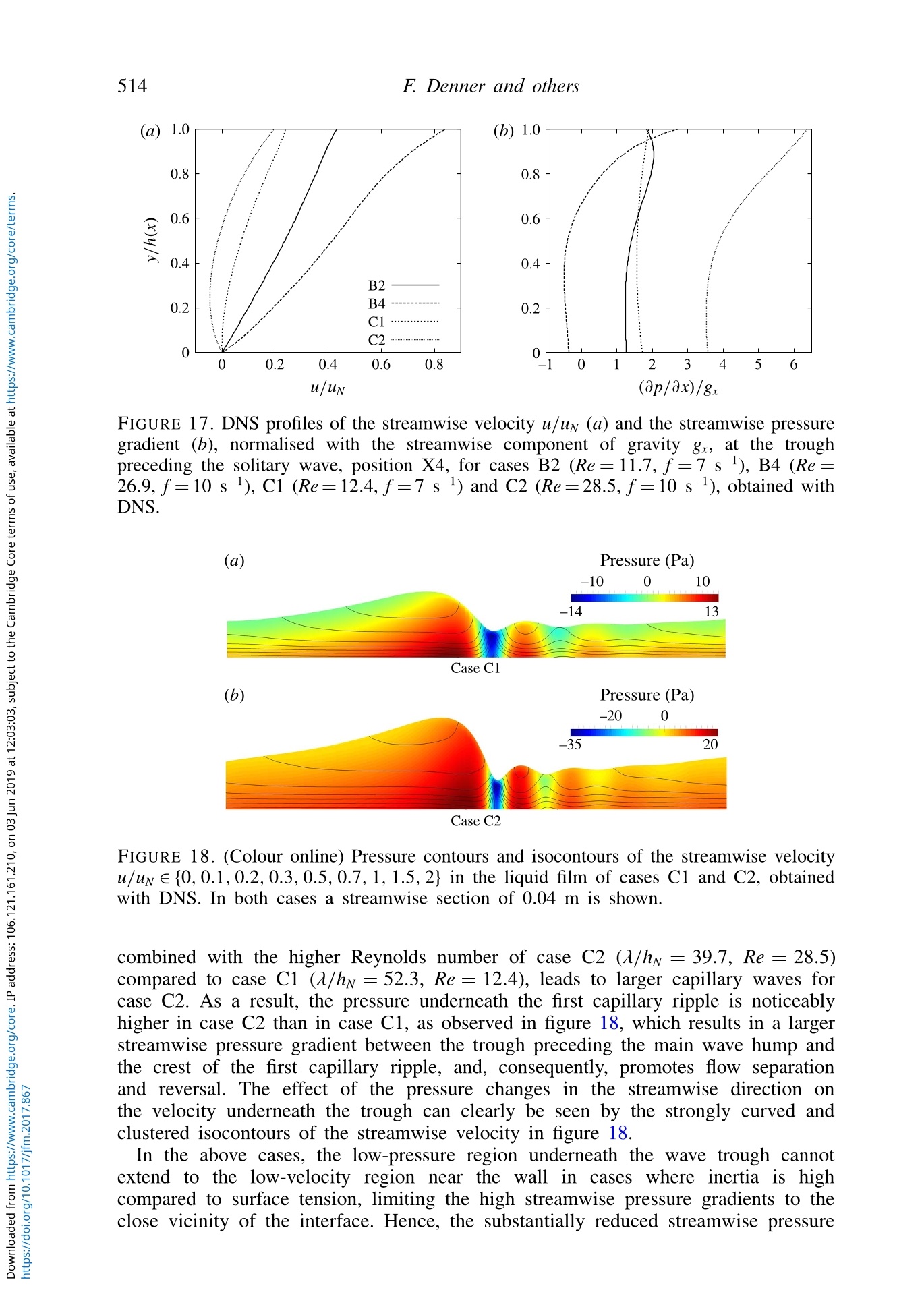
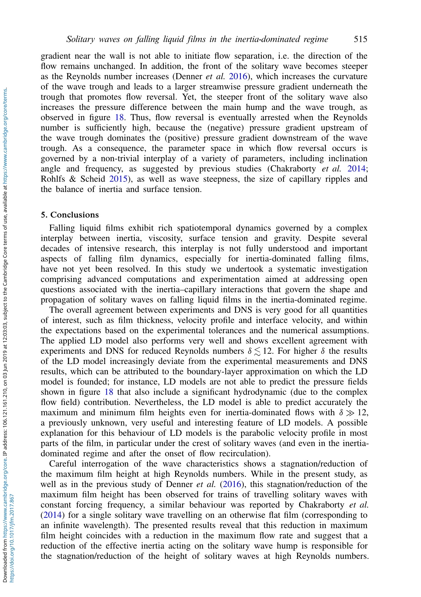
491 492F. Denner and others tEmail address for correspondence: fabian.denner@gmail.com J. Fluid Mech. (2018), vol. 837, pp. 491-519.@ Cambridge University Press 2018This is an Open Access article, distributed under the terms of the Creative Commons Attributionlicence (http://creativecommons.org/licenses/by/4.0/), which permits unrestricted re-use, distribution, andreproduction in any medium, provided the original work is properly cited.doi:10.1017/jfm.2017.867 oE33一owmooN6cmcoN9NooE3Eoo3 Solitary waves on falling liquid films in theinertia-dominated regime Fabian Dennert, Alexandros Charogiannis?, Marc Pradas23,Christos N. Markides2, Berend G. M. van Wachem,4and Serafim Kalliadasis 'Department of Mechanical Engineering, Imperial College London, London SW7 2AZ, UKDepartment of Chemical Engineering, Imperial College London, London SW7 2AZ, UKSchool of Mathematics and Statistics, The Open University, Milton Keynes MK7 6AA, UK“Chair of Mechanical Process Engineering, Otto-von-Guericke-Universitat Magdeburg, Universitatsplatz 2, 39106 Magdeburg, Germany (Received 27 March 2017; revised 25 October 2017; accepted 26 November 2017;first published online 4 January 2018) We offer new insights and results on the hydrodynamics of solitary waves on inertia-dominated falling liquid films using a combination of experimental measurements,direct numerical simulations (DNS) and low-dimensional (LD) modelling. The DNSare shown to be in very good agreement with experimental measurements in termsof the main wave characteristics and velocity profiles over the entire range ofinvestigated Reynolds numbers. And, surprisingly, the LD model is found to predictaccurately the film height even for inertia-dominated films with high Reynoldsnumbers. Based on a detailed analysis of the flow field within the liquid film, thehydrodynamic mechanism responsible for a constant, or even reducing, maximumfilm height when the Reynolds number increases above a critical value is identified,and reasons why no flow reversal is observed underneath the wave trough above acritical Reynolds number are proposed. The saturation of the maximum film heightis shown to be linked to a reduced effective inertia acting on the solitary waves asa result of flow recirculation in the main wave hump and in the moving frame ofreference. Nevertheless, the velocity profile at the crest of the solitary waves remainsparabolic and self-similar even after the onset of flow recirculation. The upper limitof the Reynolds number with respect to flow reversal is primarily the result ofsteeper solitary waves at high Reynolds numbers, which leads to larger streamwisepressure gradients that counter flow reversal. Our results should be of interest in theoptimisation of the heat and mass transport characteristics of falling liquid films andcan also serve as a benchmark for future model development. OKey words: interfacial flows (free surface), thin filmsNEOooa 1. Introduction Falling liquid films have been a topic of fundamental and applied research forseveral decades since the pioneering experiments by Kapitza (1948) and Kapitza& Kapitza (1949). A falling liquid film is a convectivelyunstable open-flowhydrodynamic system with a rich variety of spatiotemporal structures and a sequenceof wave instabilities and transitions that are generic to a large class of hydrodynamicand other nonlinear systems. Despite their apparent complexityj one can stillidentify robust coherent structures, i.e. solitary waves, in what appears to be arandomly disturbed surface. These structures interact continuously with each other asquasiparticles. Hence, a falling liquid film can serve as a canonical reference systemfor the study of spatiotemporal chaos and weak/dissipative turbulence. In addition,falling liquid films are typically associated with low flow rates, low pressure drops,small thermal resistances and large contact areas per unit volume. Not surprisingly,they play a central role in a wide spectrum of engineering applications. Prominentexamples of applications involving falling liquid films are evaporators-condensers,heat exchangers, chemical reactor columns and cooling devices. Falling liquid filmsare also exploited in saltwater desalination plants, in the food processing industry aswell as in coating processes.Furthermore, falling liquid films are found in problemsrelated to earth science and geophysics, for instance underwater gravity currents, lavaflows and the propagation of bores in rivers. Therefore, an accurate understanding ofthe hydrodynamics of falling liquid films is crucial in the design and optimisationof processes and devices that exploit these flows. The present study focuses on thehydrodynamic mechanisms that govern solitary waves on inertia-dominated fallingfilms and, in particular, on flow features that have been shown to improve the heatand mass transport characteristics of the films. 1.1. Theory and physical aspects A falling liquid film is unstable to long-wave perturbations above a critical Reynoldsnumber (Yih 1963) due to an instability mechanism that is mainly driven by shearstresses acting at the interface (Hinch 1984; Kelly et al. 1989; Smith 1990). In general,inertia and the streamwise component of gravity destabilise the flow, whereas surfacetension and the cross-stream component of gravity have a stabilising effect. A naturalsource of perturbations to a falling film flow is white noise at the inlet, wherebythe resulting instability selects the fastest growing mode of the system followed bya secondary modulation instability that converts the primary wave field into solitarywaves (Liu, Paul & Gollub 1993; Chang1994; Kalliadasis et al. 2012). Liu & Gollub(1994), however, reported regular waves by imposing a monochromatic perturbation atthe inlet in their experimental arrangement. In this case, the instability synchroniseswith the inlet forcing frequency (Liu et al. 1993; Chang1994), provided that theforcing amplitude is sufficiently large. ONEOoo芒 At low forcing frequencies, the long-wave instability develops into fast-movingsolitary waves that consist of a primary wave hump preceded by capillary ripples atthe front. These waves are predominantly two-dimensional (2D) structures (Leontidiset al. 2010), and in the inertia-dominated regime (typically for Reynolds numbers,Re ≈20-200) the velocity profile can deviate strongly from its originally parabolicshape (Malamataris, Vlachogiannis & Bontozoglou 2002; Scheid, Ruyer-Quil &Manneville 2006). In addition, if the inertia of the liquid film is sufficiently high,the maximum velocity of the fluid exceeds the wave speed of the solitary waves,leading to a recirculation zone in the moving frame (Maron, Brauner & Hewitt 1989). This zone, which appears in the main hump of the solitary waves, can considerablyimpact the heat and mass transport in the film due to the enhanced mixing (Roberts &Chang 2000; Albert, Marschall & Bothe 2014). Previous studies have found that thewave frequency, the inclination angle of the substrate, as well as viscous dispersionand capillary effects have a significant influence on the extent of the recirculationzone (Miyara2000; Rohlfs & Scheid 2015). The number of capillary ripples preceding a solitary hump increases with decreasingforcing frequency, increasing Reynolds number and decreasing viscous dispersision(Nosoko et al.1996; Pradas, Tseluiko & Kalliadasis2011), in order for surfacetension to balance inertia. Capillary ripples propagate at the same speed as the mainhump of the solitary wave (Dietze 2016), since they are continuously compressedby the main hump. As a result, faster capillary ripples have a larger amplitude(Dietze2016), in contrast to freely oscillating capillary waves which exhibit a smallerphase velocity for increasing initial wave amplitude (Denner, Pare & Zaleski 2017a).Due to the high interface curvature of the capillary ripples, pressure gradients inthe streamwise direction are significant and may lead to flow separation and localreversal of the flow direction in the laboratory frame of reference. This phenomenonwas first noted by Portalski (1964) and Massot, Irani & Lightfoot (1966), and waslater investigated in more detail in terms of the underlying mechanisms (Dietze,Leefken & Kneer 2008; Dietze, Al-Sibai & Kneer 2009) and the influence of inertia,wave frequency and inclination angle (Malamataris & Balakotaiah 2008; Chakrabortyetal.2014; Rohlfs & Scheid 2015). Numerical simulations conducted by Kunugi &Kino (2005) demonstrated a considerable enhancement of the heat and mass transportcharacteristics of the film as a result of flow reversal. 1.2. Experimental and numerical methods From an expepreirimemennttaall point of view, a range of optical (typically laser-based)methods have been developed for the investigation of the instantaneous motionand spatial extent of unsteady interfacial flows and, specifically, liquid film flows(Lel et al. 2005; Schlagen et al. 2006). Fluorescence intensity-based measurementsof the instantaneous and local film height have been conducted, for example, inlaminar falling films (Liu & Gollub1 919939;3 ;L iLu ieut al. 1993), in annular gas-liquidlows (Alekseenko et al. 2009,2012)aand in gas-sheared liquid flows in a horizontalrectangular duct (Cherdantsev, Hann & Azzopardi2014). Liu and co-workers (Liu& Gollub 1993; Liu et al. 1993) determined the critical Re for the onset of waveformation as a function of the inclination angle, and a phase boundary which separatesthe saturated, finite-amplitude wave regime from the multipeaked solitary wave regimewas identified. In the work of Alekseenko et al. (2009,2012) and Cherdantsev et al.(2014), 2D and three-dimensional (3D) film-thickness measurements were used toscrutinise the topology of large-amplitude disturbance waves as a function of Re,and to link the generation of ripples forming atop these waves to the mechanismsof liquid entrainment. Markides and co-workers (Zadrazil, Matar & Markides2014aCharogiannis, An & Markides 2015) used planar laser-induced fluorescence imaging(PLIF) instead, in order to investigate the coupling between the film-thickness andvelocity-field variations over a 2D domain. In Mathie, Nakamura & Markides (2013)and Markides, Mathie & Charogiannis (2015), the same technique was employedalongsideinfrared thermography (IR), tthusallowing for interface-temperaturemeasurementsto be retrieved simultaneously with film-thicknessmeasurements.Based on this approach,the authors reported significant heat transport enhancementsdepending on film topology. Optical velocimetry techniques can broadly be categorised depending on whethera molecular-tagging or particle-seeding approach is adopted. The photochromic dyeactivation (PDA) technique stands as a prime example of the former, allowing fordirect velocity-profile measurements via the: generation of thin fluorescing tracesarranged perpendicular to the direction of the flow (Karimi & Kawaji2000; Moran,Inumaru & Kawaji2002). Particle-image velocimetry (PIV) and particle trackingvelocimetry (PTV), instead, allow for 2D as well as 3D velocity-field characterisationby tracking the motion of seeded particle groups (PIV) or individual particles (PTV).Examples of the use of micro-PIV include the study of laminar, vertically fallingfilms (Adomeit & Renz22000) and the capillary-wave region (Dietze et al.2008).while PIV/PTV has been used, for example, in the study of downward co-currentgas-liquid annular flows (Zadrazil, Matar & Markides 2014b), where the presence ofmultiple recirculation zones within the disturbance waves was revealed. In terms of modellingaand computational methodologies, a substantiall numberof studies have focusedon low-dimensional (LD) formulations, which simplifythegoverning equations and associated wall and free-surface boundary conditionsconsiderably. Using the long-wave expansion, a hierarchy of model equations hasbeen obtained, starting from the so-called Benney equation (Benney1966) whoseregion of validity is restricted to near-critical conditions (Kalliadasis et al. 2012), tointegral-boundary-layer equations which are valid away from criticality and describethe evolution of both the film height h and the local flow rate q (Shkadov 1967) (seealso the work by Scheid et al. (2006), where different LD models are compared toeach other). Numerical modelling has also received considerable attention, with directnumerical simulation (DNS) finding increasing application in the study of fallingliquid films. The work of Ramaswamy, Chippada & Joo (1996) was the first DNSstudy to conduct a detailed investigation of this problem, focusing on the stability offalling films as well as on the development and interaction of interfacial instabilities.Subsequently, Malamataris et al. (2002) showed that the velocity profile of the liquidfilm is strongly non-parabolic in solitary waves, whereas studies of Gao, Morley &Dhir (2003) and Nosoko & Miyara (2004) investigated the dynamics of periodicallyperturbed falling films at different forcing frequencies and Reynolds numbers. Acommon assumption made in the majority of computational studies is a periodiccomputational domain in which the film thickness is conserved, hence increasing theflow rate at the onset of interface waves (Ramaswamy et al. 1996; Gao et al. 2003)and imposing a particular wavelength on the instabilities (Kalliadasis et al. 2012). Inreality, however, the system is not closed but open and, therefore, it is not the meanfilm thickness but the mean flow rate that is conserved, resulting in a decrease of theaverage film thickness for wavy film flows (Chang, Demekhin & Kalaidin 1995; Gaoet al. 2003). Numerical studies using periodic domains are, hence, limited in theirability to accurately predict spatiotemporally evolving interface instabilities. 1.3. Objectives ONEOoo芒 Despite the significant number of studies focusing on the hydrodynamics of solitarywaves on falling liquid films, most of which have been conducted in the region ofsmall-to-moderate Reynolds numbers (Re ≤20), a number of open questions regardingthe hydrodynamics of inertia-dominated solitary waves still remain. Previous DNSstudies (Chakraborty et al. 2014; Denner et al. 2016) have reported results in whichthe wave height stagnates, meaning it stays approximately constant, or reduceswhen increasing the Reynolds number above :a critical1 value. Considering that oE33一owmooN6cmcoN9NooE3Eoo3 the wavelength of solitary waves increases for larger Reynolds numbers (Denneret al. 2016), a yet unidentified mechanism must be responsible for the saturation(stagnation or reduction) of the height of solitary waves. Similarly, with respect tothe flow reversal observed underneath the trough preceding the solitary wave, thehydrodynamic mechanisms responsible for the upper limit in Reynolds number abovewhich no flow reversal was observed in simulations of Chakraborty et al. (2014)have yet to be explained. It is also worth noting that none of the previous studiesincluded a detailed and systematic comparison between experimental measurementsand numerical results using LD models or DNS. If such a comparison confirms goodagreement, a concurrent application of these methods may provide more detailedinsight into the complex hydrodynamics of solitary waves. Aiming to provide answers to these open questions, synergisticapproach with a combination of experiments, DNS as well as LD modelling. Adirect comparison of experimental and numerical results is instrumental in assessingthe predictive quality of the available computational methods and in analysing theflow field and wave characteristics in detail. We find that experimental measurementsand DNS results agree very well, in particular with respect to film height and flowvelocity at the interface, while the applied LD model is favourably compared withboth of them. Of particular interest in our study is the flow field within the fallingliquid films and its influence on the dynamics of solitary waves and capillary ripples,in order to elucidate the mechanisms stabilising the wave height and influencing theflow separation and reversal at large Reynolds numbers. The presented experimentaland numerical results can also sererveas ahydrodynamics of falling liquid films. In 2 the characterisation of falling liquid films and the associated solitary wavesis discussed. In $3 we introduce the experimental and numerical methods we adoptand detail the case studies we undertake. The results are presented and discussed in$4 and conclusions are offered in 5. 2. Characterisation of falling liquid films Consider a film flowing down a planar inclined plane forming an angle p with thehorizontal direction, as shown in figure 1. There exists a spatially uniform solution,often referred to as the Nusselt flat-film solution (Nusselt 1916), with film height and average film velocity where pi and p are the dynamic viscosity and the density of the liquid film,respectively, qn = uwhy is the flow rate per unit span and g is the gravitationalacceleration. Based on this idealised solution, various characteristic scalings can beformulated. EON NuO 2.1.sselt scaling oo 芒 Making use of the representative pressure scales of the three major hydrodynamicmechanisms acting on the falling film (inertia, viscous stresses and surface tension) FIGURE 1. Sketch of the profile geometry for a liquid film on a substrate with inclinationangle β to the horizontal. h(x,t) is the local film thickness with respect to a Cartesiancoordinate system (x,y), with x the streamwise coordinate and y the outward-pointingcoordinate normal to the substrate. several dimensionless parameters can be defined. The Reynolds number expresses the relative importance of inertia over viscous effects, the Weber number where o is the surface tension, represents the relative importance of inertia to surfacetension, and the capillary number, a measure of the relative importance of viscous stresses and surface tension. TheReynolds number Re can also be regarded as the dimensionless flow rate. Thesenon-dimensional numbers are related to each other by We = Re Ca and are oftenreferred to as Nusselt scaling in the context of falling liquid films, because theyare based directly on the Nusselt flat-film solution. Numerical results presented byDenner et al. (2016) suggest that the capillary number is not suitable to characteriseinertia-dominated solitary waves. Denner et al.((22001166)) recently proposedan ‘inertia-corrected scaling’for thecharacterisation of solitary waves on falling liquid films based on the driving Nusseltvelocity uy =uy sin B. Using this velocity scale, the Reynolds and Weber numbersare redefined as Re*=Re sinB and We*= We(sin B)2,respectively, which was shownto lead to a self-similar characterisation of the shape and dispersion of solitary waveson falling water films for a given inclination angle of the substrate and forcingfrequency. Unlike the dimensionless numbers above, which depend on the flow rate, theKapitza number where v=wi/p is the liquid kinematic viscosity, depends only on the properties ofthe liquid and inclination angle B. Hence, for a fixed liquid and B, the Kapitza numberis fixed and the only free parameter is the Reynolds number. Solitary waves on falling liquid films in the inertia-dominated regime 2.2. Shkadov scaling Following the scaling introduced by Shkadov (1977), a reduced Reynolds number and the viscous dispersion number can be obtained. This reduced Reynolds number 8 compares inertia and viscouseffects at the length scale imposed by surface tension and gravity. On the other hand,the viscous dispersion number n appears along with every second-order streamwiseviscous term in the momentum equation and has a dispersive effect on the speed oflinear waves (Pradas et al. 2011; Kalliadasis et al. 2012). The Shkadov scaling isparticularly useful for the characterisation of LD models, as further discussed withrespect to the applied LD model in $3.3. Based on the reduced Reynolds number 8, Ooshida (1999) identified two regimes:the drag-gravity regime for 81 and the drag-inertia regime for 81. In the drag-gravity regime, the flow is similar to that of the Nusselt flat-film solution, with bothinertia and surface tension playing effectively a perturbative role (Kalliadasis et al.2012). In the drag-inertia regime on the other hand, inertia and surface tension are nolonger corrections to the Nusselt flow, the cross-stream velocity component becomessignificant and the velocity profile of the film flow can become strongly non-parabolic(Malamataris et al.2002). Recent studies (Chakraborty et al. 2014;Rohlfs & Scheid2015) found the transition between the drag-gravity and drag-inertia regimes to occurat 1 <8 ≤6. Additional effects - for example, shear-thinning and non-Newtonianbehaviour - can lead to complex behaviour in the vicinity of this transition (such ashysteresis) (Pradas et al. 2014). 3.Methods 3.1. Experimental methodology ONEOoo芒 The experimental apparatusand methodologies developed to generatee tthe filmthicknessand velocity data have been described extensively in ourpreviouspublications (Charogiannis et al. 2015,2017), and therefore only a summary ispresented here for the sake of clarity and completeness. A schematic of theexperimental arrangement, itself an evolution of a previously developed set-up (Mathieet al. 2013; Markides et al. 2015), is depicted in figure 2. The apparatus consistsof a main test section over which film flows develop, and a closed loop via whichthe liquid circulates. Prior to entering a flow-preparation distribution box, the flowis split into a steady supply g and a pulsating supply . The latter is generatedby an oscillator valve that allowss accurate control of the forcing frequency andamplitude to be achieved, selectively triggering the rapid growth of fully developedwave regimes within the confines of our test section. The instantaneous flow rate intothe distribution box is calculated from the output signal of an ultrasonic flowmeter.The role of the distribution box is to create a well-characterised uniform flow with low noise levels, and to introduce this over the test section with uniform thickness. FIGURE 2. (a) Schematic of the test section and part of the flow loop. (b) Test sectionarrangement showing the position of the cameras and illuminated region of the film(Charogiannis et al. 2015,2017). 3.1.1. Test section and imaging arrangement The test section comprises a thin soda-lime glass plate with 0.7 mm thickness,mounted on an aluminium support frame and inclined at 20°to the horizontal.The Reynolds number can be evaluated at the flow inlet using the mean flow-ratemeasurement per unit width of the channel Q, as where Ubox is the bulk velocity inside the box and D is the channel depth. Afrequency-doubled Nd:YAG laser (532 nm) is used to illuminate the flow, which isseeded with Rhodamine B dye for PLIF and glass-hollow-sphere particles for PIV, at asampling rate of 100 s-. Sheet optics are employed in forming a thin (approximately0.1 mm) laser sheet extending along the (streamwise) length of the substrate, while apair of LaVision HS 500 CMOS cameras equipped with Sigma 105 mm f/2.8 Macroenses are employed to achieve the desired magnification (between 28.0 um and29.7 um per pixel depending on Ka). Excitation of the dye-doped liquid and imagingof the emitted fluorescence is performed from underneath (unwetted side), in orderto avoid spatially and temporally non-uniform beam stirring and lensing in the firstinstance, and to limit image distortions in the latter. The imaging planes of the twocameras are mapped using a calibration graticule target immersed inside the liquidsolution. Optical distortion corrections are performed using the same arrangement,and a pinhole model available in LaVision DaVis. 3.1.2. PLIF/PTV data acquisition and processing A sample PLIF frame after correction for perspective distortion is (depicted infigure 3(a). Near the solid-liquid interface, reflections from the substrate blur thePLIF signal locally, while the fluorescence emitted by the illuminated liquid volumeis reflected about the liquid-gas interface and back to the camera. The location ofthe solid-liquid interface is obtained using an edge-detection algorithm, while forthe gas-liquid interface, intercepts between linear fits to maximum signal gradientsand reflection intensity profiles are employed as estimates of the liquid boundaries. (a) Raw LIF image (b) oE33一owmooN6cmcoN9NooE3Eoo3 (c) Raw particle image (d) Distance along the film, x(mm) Distance along the film, x (mm) FIGURE 3. (a) PLIF image from a flow with Re=62, Ka=350 andf=10 s-, followingcorrections for refractive-index and perspective distortions, and (b) binarised PLIF imageafter removal of out-of-plane reflections. (c) Particle image from a flow with Re =24,Ka=85 and f=10 s- after corrections for refractive-index and perspective distortions,and (d) masked-particle image using its processed PLIF counterpart. The processed profiles are then used to mask out the reflection regions and to producebinarised images (see figure 3b), where a signal intensity of unity corresponds to thefilm domain and a signal intensity of zero is ascribed to the rest of the image. ONEOoo The binarised images are used to mask out reflections from the glass surfaceunderneath the liquid domain and about the gas-liquid interface in the raw particleimages (see figure 3c,d). A four-pass cross-correlation algorithm is implementedon the masked-particle-image sequences in order to generate 2D velocity-vectormaps (PIV calculation). Following this step, individual particles are tracked (PTVcalculation) by employment of the obtained PIV results as reference estimators of thevelocity field. There are a number of reasons for employing PTV rather than PIV inthis study. To begin with, PTV offers an eight-fold increase in the spatial resolutionof the velocity measurement based on the selected velocity-vector calculation settings(which are determined based on the optical set-up, the size of imaged region ofthe flow and the employed particles). A second reason is that PIV suffers fromlarge bias errors in the presence of strong velocity gradients, as the motion ofparticle groups is averaged within the PIV interrogation window. Along a smoothfilm region and near the gas-liquid interface this effect is of little consequence, andPTV and PIV produce similar results. Near the wall, however, as well as betweenthe wave crests and troughs, and along the capillary-wave regions, where the velocityvaries strongly over a limited spatial domain, PIV falls short of providing crediblequantitative results. It should finally be noted that the presence of particle-imagereflections within the masked liquid domain constitutes a commonly encountered errorsource affecting the PTV velocity data (Kaehler, Scholz & Ortmanns 2006; Kaehler, Distance along the film,x(mm) FIGURE 4. (a) Reference and average-wave profiles for a film with Re=26.9, Ka=85and a 10 s- forcing frequency. (b) Average PTV-derived velocity field corresponding tothe average film-thickness profile in (a). Scharnowski & Cierpka 2012). In our experiments, a spatial extent correspondingto only approximately 5%-7% of the examined films is strongly affected by suchartefacts, and consequently, the impact on bulk velocity measurements is minimal. For a detailed examination of the velocity distributions underneath the waves,the practice of averaging PTV maps corresponding to the same spatial region isadopted. The procedure is initialised by selecting a reference film-thickness profilepertaining to the desired topology, and cross-correlating it with all thickness tracesfrom the same data set. Signal pairs satisfying a maximum displacement conditionare then repositioned and averaged (a typical result is shown in figure 4a). Thesame translation values are used to rearrange and average out the correspondinginstantaneous PTV velocity maps, producing averaged velocity fields such as the onedisplayed in figure 4(b). 3.1.3. Validation Independent experiments are conducted in order to assess the validity and accuracyof the combined optical methodology. Film thicknesses from flat films (Ka=14) arecompared to predictions from the Nusselt flat-film solution and direct micrometre-stage measurements. In both cases the mean relative-deviation amounts to below 1 %.The same uncertainty value is believed to apply to wave-locked average measurementsof mean film thickness; however, thinner films ensue in that case, and consequentlya worst-case uncertainty of 2% is a more representative estimate. An estimate of thefilm-thickness measurement noise is obtained by calculating standard deviations overa wide range of flat-film datasets. This amounts to <30 um, and therefore, a meanrelative error of 2.5 % is quoted for the instantaneous film-thickness measurements. ONEOo Relative deviations are also calculated between PTV-derived interfacial and bulkvelocities, and corresponding analytical results of the Nusselt flat-film solution, withaverage relative deviations corresponding to 3.2% for both velocities. Standarddeviations of local velocity in flat films (conservative estimates of PTV measurementnoise)are observed to decrease with increasing distance from the wall;: at thegas-liquid interface, they typically amount to less than 1% of the local mean value,while halfway across the film thickness they amount to approximately 5%-6% ofthe mean value. 3.2. DNS methodology The applied DNS methodology is based on a general-purpose finite-volume frameworkfor interfacial flows (Denner & van Wachem 2014a), which resolves the dynamics ofthe full two-phase system, i.e. the liquid film, the gas-liquid interface and the gasphase. The flow, which is assumed to be incompressible and isothermal, is governedby the momentum equations and the continuity equation where t represents time, u is the velocity, p is the pressure, p is the density, uis the dynamic viscosity, g is the gravitational acceleration and )8fo represents thecontribution of the surface tension. 3.2.1. Numerical framework Theprimitive variablesare obtained.1usinga coupled, implicit finite-volumeframework with collocatedvariable arrangement (Denner & van Wachem22014a).The momentum equations (3.2) are discretised using a second-order backward Eulerscheme for the transient term, while the convection, diffusion and pressure terms arediscretised using central differencing. The continuity equation (3.3) is discretised usinga balanced-force implementation of the momentum-weighted interpolation method, asproposed by Denner & van Wachem (2014a), which couples pressure and velocity. The volume-of-fluid (VOF) method (Hirt & Nichols1981) is adopted to capturethe gas-liquid interface. In the VOF method the local volume fraction in each cell isrepresented by the colour function y, defined as y=0 in fluid a and y=1 in fluid b.Hence, the interface is located in mesh cells with a colour function value of 0 < y <1.The colour function is advected by the linear advection equation which is discretised using a compressive VOF methodology (Denner & van Wachem2014b). Assuming surface tension is a volume force acting in the interface region,the surface force per unit volume is described by the continuum surface force (CSF)model (Brackbill, Kothe & Zemach1992) as fo =ok Vy, where k represents theinterface curvature. The artificial viscosity model for interfacial flows of Denner et al.(2017b) is also applied to mitigate the impact of parasitic and spurious flow featureson the numerical solution. 3.2.2. Simulation set-up ONEOoo芒 The applied two-dimensional computational domain, illustrated in figure 5, has thedimensions L x Ly, where Ly= 4hy and the domain length L=0.256 m + 50hyis chosen to allow a direct comparison with the corresponding experimental resultsat the experimental measurement point xm =0.256 m downstream from the inlet.The additional domain length of 50hw is taken to be sufficiently long so astoensure that the outlet of the computational domain does not affect the flow fieldand interface instabilities in the measurement region. The computational domain isrepresented by an equidistant Cartesian mesh with a resolution of 10 cells per filmheight hy. The time step At satisfies a Courant number of Co=|u|△t/▲x≤0.25 aswell as the capillary time-step constraint derived by Denner & van Wachem (2015). FIGURE 5. Schematic illustration of the numerical domain with dimensions(L×L). Theliquid film with height h(x, t) flows from the left to the right on an inclined substrate. The properties of the liquid film are directly taken from the experimental measure-ments(see 83.4) and the gasphase isassumed to be air with density =1.205 kg m-3 and viscosity wg=1.82×10⁻⁵ Pa s. At the bottom (liquid-side) wall a no-slip condition is enforced and at the top (gas-side) boundary a free-slip wall is applied. A monochromatic forcing is imposed atthe domain inlet by periodically changing the mass flow at a given frequency f andamplitude A from the mean. A semiparabolic velocity profile is prescribed for theliquid phase at the inlet and a spatially invariant velocity is prescribed at the inlet of the gas phase, given as The co-flow in the gas phase is applied to prevent backflow at the domain outlet,which can significantly affect the computational performance as well as the accuracyof the results, but has a negligible effect on the evolution of the film flow, sincethe momentum of the gas phase is approximately three orders of magnitude smallerthan the momentum of the liquid film. A constant film height h(x=0) = hy isprescribed at the inlet. An open boundary condition is applied at the domain outlet,as previously used for instance by Nosoko & Miyara (2004) and Demekhin et al.(2007) (Kalliadasis et al. (2012, appendix F3) gives details on how to apply an outletboundary condition). 3.3. LD modelling We adopt the LD formulation corresponding to the two-field second-order modelderived by Ruyer-Quil & Manneville (1998), a set of two coupled nonlinear equationsfor the evolution of the interface thickness h(x,t) and local flow rate q(x, t): 8- /9q0h where the Shkadov scaling (Shkadov 1977) has been used, giving rise to the reducedReynolds number 8 defined in (2.7) and the viscous dispersion number n definedin (2.8). The above model is obtained by combining the long-wave expansion upto second order with a weighted residual technique based on a Galerkin projectionin which the velocity field is expanded onto a basis with polynomial test functions(Ruyer-Quil & Manneville 1998,2000, 2002) (this formulation was extended to 3Din the study by Scheid et al. (2006)). It is worth remarking that the model containsthe second-order viscous dispersion terms (those gathered in the second line of (3.7)),which are controlled by n, often neglected in thin-film studies. These terms affect boththe amplitude and frequency of the capillary ripples at the front of solitary waves(Ruyer-Quil & Manneville 2000). The first-order model, obtained by setting n= 0in the second-order one already corrects the shortcomings of the first-order modelobtained by Shkadov (1967), with the principal one being an erroneous prediction ofthe instability onset, while the second-order model is in good agreement with Orr-Sommerfeld for a sufficiently large region of Re. Also, as was demonstrated by Pradas et al. (2011), who developed a coherent-structure theory for falling films, the second-order terms play an important role in theinteractions between solitary pulses precisely because they affect both the amplitudeand frequency of the front-running capillary ripples, and hence they are crucial foran accurate description of pulse interaction. So their influence is in fact linear, butthey can have profound consequences on the nonlinear dynamics of the film andthe wave-selection process in the spatiotemporal evolution. This is because solitarywaves interact through their tails which overlap, i.e., the capillary ripples and theiramplitude and frequency will affect the separation distance between the pulses: forinstance, smaller-amplitude ripples will allow for more overlaps between the tails ofneighbouring solitary waves, thus decreasing their separation distance. This in turnwill affect the average separation distance between the waves when the system reachesits permanent quasiturbulent regime, and hence the density of the solitary waves. Equations (3.7) and (3.8) are solved numerically by making use of a variable time-step Runge-Kutta method with a central finite difference technique in space. A typicaltime step is △t=0.0025 and the domain [0, L] with L=150 is discretised into 2000intervals. At the inlet of the system we impose an inflow boundary condition, given as and like with our DNS we impose an open-soft boundary condition at the outletof the system to minimise any reflections (again, appendix F3 in Kalliadasis et al.(2012) gives details on how to do this). The initial condition is given as the flat-filmsolution with h(x,0)=1. 3.4. Investigated case studies We consider cases with Reynolds numbers in the range Re= 5.1-77 and Kapitzanumbers in the range Ka=14-346 with the relevant parameters given in table 1. Theworking fluid for the experiments is an aqueous glycerol solution with three differentglycerol concentrations (by weight) X : ONECases A: X=82%, p=1214 kg m-3,u=7.49×10⁻² Pa s and o=0.0623 N m-l,Ooo芒 Cases B: X=65%,p=1169 kg m-3,w=1.84×10⁻² Pas and o=0.0587 N m-l, Cases C: X=45%, pi=1113 kg m-3, wi=6.42×10⁻³Pa s and o=0.0597 N m-. oE33一owmooN6cmcoN9NooE3Eooc3 FIGURE 6. Schematic illustration of the positionsat wyhich profiles of velocityandpressure gradients are analysed. Position X2 is located at the crest of the solitary waveand position X4 is located at the trough preceding the solitary wave. Case f (s-) Re We 8 A1 5 5.1 0.75 11.7 0.58 A2 7 5.2 0.76 11.8 0.58 B1 7 7.5 0.24 10.3 0.21 B2 7 11.7 0.49 17.6 0.25 B3 7 20.6 1.26 35.0 0.32 B4 10 26.9 1.98 48.8 0.37 C1 7 12.4 0.13 11.8 0.10 C2 10 28.5 0.53 32.7 0.15 C3 7 45.1 1.15 57.3 0.18 C4 7 65.1 2.11 89.9 0.21 C5 10 65.7 2.09 89.2 0.21 C6 7 77.0 2.79 110.3 0.23 TABLE 1. Forcing frequency and non-dimensional parameters of the analysed cases. OEoo To allow a direct comparison of the experimental and numerical results, all cases areanalysed at downstream distance xm=0.256 m from the inlet of the test domain, asdictated by the employed experimental arrangement. The experiments are conductedfirst by choosing the amplitude of the monochromatic inlet forcing so that fullydeveloped, quasistationary interface waves are obtained at the measurement positionxm = 0.256 m. Subsequently, the numericalsimulations are conducted using themeasured fluidproperties and flow rate as well as the imposed monochromaticforcing frequency and forcing amplitude in the experiments, thus establishing a directcomparison under the same conditions. The presented velocity profiles are taken atthe positions illustrated in figure 6, where d is the distance between the crest of thesolitary wave and its preceding trough. Figures 7 and 8 show the spatial development of the film height and the streamwisevelocity at the interface for cases A2 and C6, respectively, obtained with DNS. The Solitary waves on falling liquid films in the inertia-dominated regime x(m) FIGURE 7. Spatial development of the film height h/hy and the streamwise velocity at theinterface uy/un for case A2 (Re=5.2), obtained with DNS. The minimum and maximumvalues at the measurement position (xm=0.256 m) are shown as a reference by the dashedgrey lines. x(m) FIGURE 8. Spatial development of the film height h/hy and the streamwise velocity at theinterface uy/uy for case C6 (Re=77.0), obtained with DNS. The minimum and maximumvalues at the measurement position (xm=0.256 m) are shown as a reference by the dashedgrey lines. figures reveal that in the studied range of Reynolds numbers the solitary wavesare fully developed at the measurement position xm. Furthermore, in both cases thedifference in wave speed at the trough and the crest of the solitary wave is <0.1 %,indicating that the waves have stopped growing. 4. ResultsONEOoo 4.1. Comparison of experimental and numerical results The experimental measurements and numerical predictions of the film height h andstreamwise interface velocity uy as a function of downstream distance x are shownin figures 9 and 10 for selected cases. The DNS results are generally in very goodagreement with the experimental ones, both in terms of film height and interface F. Denner and others oE33一owmooN6cmcoN9NooE3Eoo3 FIGURE 9. Instantaneous film height h, normalised with the Nusselt flat-film height hy,for selected cases as a function of downstream distance x. FIGURE 10. Instantaneous streamwise interface velocity uy, normalised with the Nusseltvelocity un, for selected cases as a function of downstream distance x. The wave speedsmeasured in the experiments, cEx, and the DNS, cpns, are given as well. ONEOoo velocity, similar to previously reported comparisons between experiments and DNSby Dietze & Ruyer-Quil (2013), using the open-source software GERRIS, and byDoro & Aidun (2013) and Rohlfs, Pischke & Scheid (2017), using the open-sourcesoftware OPENFOAM. The LD model is also in very good agreement w thexperimental and DNS results provided that 8≤12, but fails to capture the amplitudeand frequency of the front-running capillary ripples for 8 > 12 (which in turn affect oE33一owmooN6cmcoN9NooE3Eoo3 FIGURE 11. Maximum film height hmax/hy (a), minimum film height hmin/hy (b) andwave speed c/un (c) as a function of Re for cases with f=7 s-. Results obtained withthe LD model are omitted in the interest of clarity. the separation distances between the solitary waves) even though it includes thesecond-order viscous dispersion effects. In particular, both the DNS and experimentalresults show fewer capillary ripples with increasing inertia than the LD model(compare, for example, cases C1 and C6 in figure 9). Such a deviation is neverthelessexpected since cross-stream inertia is not negligible for 8>1 (Kalliadasis et al. 2012),thus violating one of the main assumptions in the boundary-layer approximationinvoked to obtain the LD formulation. Interestingly, however, the LD solutioncaptures very well the primary solitary hump, including the maximum and minimumfilm heights, in all studied cases (8=10.3-110)- a fact not previously reportedin the literature. The maximum film height hmax, minimum film height hmin and wave speed cobtained from the experiments and DNS, shown in figure 11 for all considered caseswith forcing frequency f=7 s-, are generally in satisfactory agreement with eachother. In particular, the same trends can be extracted with respect to the change infilm height and wave speed as Re increases. An increase in Re causes initially anincrease in wave height, irrespective of the Kapitza number Ka, both with respectto the Nusselt flat-film height hy and the film height in the preceding trough hmin.Eventually, the normalised maximum film height shown in figure 11(a) reaches amaximum with respect to Re. Increasing Re further ensues a decrease in maximumfilm height, as already noted in previous studies (Chakraborty et al. 2014; Denneret al. 2016). Interestingly, the observed trend persists for the wide range of Kapitzanumbers Ka considered in this study, with Ka=14-346 in figure 11, both in theexperimental measurements as well as the DNS results. The minimum film heighthmin shows a similar yet inverse behaviour compared to the maximum film heightas far as the influence of Re is concerned, similar to the observations reported byDenner et al. (2016) for falling water films. ONEOo Figure 112compares the profiles of the dimensionless streamwise velocity u/uyin the liquid film at different positions in the solitarywave, for selectedcasesThe agreement between experimental measurements and DNS results is in generalvery good, especially for the small Reynolds numbers, cases A1 (Re =5.1) andB1 (Re=7.5). At larger Reynolds numbers the flow field is strongly dependent onthe local wave shape and can vary rapidly in space, as shown by the experimentalmeasurements of Charogiannis et al. (2017) for instance. Hence, in particular at thefront of the solitary wave (see figure 12c), small differences in local film heightand measurement position can lead to noticeable differences in the velocity profile.Note that the velocity profile is parabolic in the tail and underneath the crest of the —-— Experiment -..DNS (a) oE33一owmooN6cmcoN9NooE3Eoo3 0 2 0 2 0 2 0 2 0 2 u/un u/uy u/un u/un u/un FIGURE 12. Comparison of the experimental and DNS velocity profiles in the tail, atthe crest and at the front of the solitary wave for selected cases, normalised with thecorresponding Nusselt flat-film velocity un and the local film thickness h(x). (a) In the tailof the solitary wave, see position X1 in figure 6. The circular dots indicate a semiparabolicvelocity profile. (b) At the crest of the solitary wave, see position X2 in figure 6. Thecircular dots indicate a semiparabolic velocity profile. (c) At the front of the solitary wave,see position X3 in figure 6. ONEOoo solitary wave, even for the case with the highest Reynolds number (case C6, Re=77).This agrees with previously reported numerical results (Malamataris et al. 2002;Gao et al. 2003; Malamataris & Balakotaiah 2008) and experimental measurements(Adomeit & Renz 2000; Moran et al. 2002; Charogiannis et al. 2015). Interestingly,the self-similarity of the velocity profile in the laboratory frame of reference isunaffected by the onset of a recirculation region in the moving frame when themaximum flow velocity exceeds the wave speed (for instance, in case C6). Movingfurther downstream to the front of the solitary wave, position X3, the velocity profileincreasingly departs from the parabolic one that is observed for the tail and the crestof the solitary wave, as clearly seen in figure 12(c). The limitations of the appliedPIV/PTV method to measure the velocity fields in our experimental arrangementprohibit a direct comparison of the velocity profiles obtained experimentally withthose from DNS in the trough of the solitary wave (position X4). In summary, carefully conducted experiments3and DNS using state-of-the-artmethods show good agreement when predicting harmonically excited solitary waves on falling liquid films in the inertia-dominated regime and not only for flows withsmall Reynolds numbers reported in previous studies (for example, Gao et al. (2003),Dietze & Ruyer-Quil (2013)). Note that this comparison of experiments and DNS ismore detailed than previously published comparisons (notably Dietze & Ruyer-Quil(2013), Doro & Aidun (2013), Rohlfs et al. (2017)), as it comprises the film height,film velocity at the interface, the velocity profile in the liquid film at differentpositions, and the wave speed, across a range of Reynolds and Kapitza numbers.This allows one to draw conclusions based collectively on both the experimentalmeasurements and the DNS results. And although the LD model is applied outsidewhat is usually considered to be its range of validity (8≤10), its predictive accuracywith respect to the maximum and minimum film height, and consequently the waveheight, is impressive and somewhat unexpected. This might be explained by thepredominantly parabolic velocity profile in the tail and underneath the crest of thesolitary wave, which accounts for the largest part of the solitary wave, even after theonset of flow recirculation. 4.2. Mechanism for stabilising the wave height A reduction of the maximum film height with increasing Re is observed in figure 11(a)in the experimental measurements as well as the DNS results. Chakraborty et al.(2014) also reported a reducing maximum film height in their DNS results of aliquid film (Ka=193-10000) with a single solitary wave on a vertical substrate,for sufficiently high reduced Reynolds numbers 8. Similarly, Denner et al. (2016)reported a stagnation of the maximum film height for sufficiently high Reynoldsnumbers on substrates with different inclination angles β=45°-90°and using fluidswith different surface tension coefficients. Extending the balance ofgravity andviscous stresses (which forms the basis of the Nusselt flat-film solution) to wavyfilms, the film height is related to the Reynolds number as h~√Re. Thus, the waveheight should increase with increasing Reynolds number, instead of stagnating oreven reducing, as suggested by the presented numerical results and experimentalmeasurements. Surface tension stabilises the wave, yet the absolute value of theinterface curvature of the main wave hump is decreasing for increasing Reynoldsnumber once the wave height does not further increase, since the wavelength of thesolitary wave is 1~√Re sin B (Denner et al. 2016). Hence, the surface tension actingon the solitary wave decreases with increasing Re. Consequently, there must be analternative mechanism acting to stabilise the height of the solitary wave against thedestabilising effect of the increased inertia. Figure13shows the maximum film height hmax, normalised by the Nusselt heighthw, alongside the corresponding maximum flow rate qmax, normalised by the Nusseltflow rate qn, for cases with Ka= 346 (cases C) and f= 10 s-, in the Reynoldsnumber range Re= 10-85, obtained with DNS. The instantaneous local flow rate isdefined as where h(x) and u(x) are the local film height and flow velocity, respectively. Bothhmax/hy and qmax/qn exhibit a clear maximum with respect to the Reynolds numberat Rec ≈ 50, and decrease for further increasing Reynolds number Re> Rec, as isevident in figure 13. A similar behaviour is observed comparing hmax/hy and qmax/qvof a water film falling on a vertical substrate, as previously considered by Denneret al. (2016), shown in figure 14. Charogiannis et al. (2017) recently established a Re Re FIGURE 13. Maximum film height hmax (a) and maximum flow rate qmax (b), normalisedby the corresponding Nusselt solution, as a function of Reynolds number Re for case Cwith f=10 s-l, obtained with DNS. linear relationship between local flow rate and local film height for a given solitarywave, with a slope that correspondsincrease and decrease of hmax/hw and qmax/qv observed in figures13aand14 is tobe expected. Moreover, the shape of the solitary wave is governed by the balanceof inertia, represented by the dynamic pressure pdyn = pu/2, and surface tension,represented by the capillary pressure po =o/hw (Denner et al. 2016). The relevantcharacteristic parameter is, thus, the Weber number We=2pdyn/po (see (2.4)), whichcan be rewritten with respect to position x as based on the local flow rate given in (4.1). Since the density pi and surface tensioncoefficient o are assumed to be constant, a change in flow rate leads to a change infilm height at a given Weber number. Note that the dynamic pressure pdyn representsthe (streamwise) translational kinetic energy Eu=mu/2 per unit volume of the liquidfilm. where m is the fluid mass. ONEOoo A plot of the maximum film height against the maximum flow rate, presentedin figure115(a), confirms the correlation between hmax/hw and qmax/qw establishedabove, but it also shows a reduction of the maximum flow rate corresponding to agiven maximum film height for Re > Rec. This difference between qmax at a givenhmax for Re Ree suggests a reduction ofthe effective inertia acting on the solitary wave for Re> Rec, with Ree~ 50 for theconditions analysed in figure 15(a). Interestingly, this reduction of effective inertiacoincides with the development of flow recirculation in the main wave hump withrespect to the moving frame of reference when the maximum flow velocity surpassesthe wave speed, umax > c, as observed in figure 15(b). The flow recirculation inthe moving frame of reference increases the angular velocity and, as a result,increases the angular kinetic energy EQ=I22/2, where I is the moment of inertia.Due to the conservation of energy, the increase of angular kinetic energy E reducesthe translational kinetic energy Eu. This transfer of energy leads to the observedreduction in effective inertia of the film flow. It is worth noting that the increase in oE33一owmooN6cmcoN9NooE3Eoo3 FIGURE 14. Maximum film height hmax (a) and maximum flow rate qmax (b), normalisedby the corresponding Nusselt solution, as a function of Reynolds number Re for a fallingwater film on a vertical substrate, as previously considered in Denner et al. (2016),obtained with DNS. ·80 70 60 50 40 30 20 10 FIGURE 15. (Colour online) Maximum flow rate gmax (a) and relative velocity umax -c (b),normalised by the corresponding Nusselt solution, as a function of maximum film heighthmax for case C with f=10 s- in the range Re=10-85, obtained with DNS. The colourscale represents the Reynolds number. ONEOoo corresponds to an increase in vorticity ω=22 (assuming incompressible flow andneglecting high-order contributions). However, an analysis of the vorticity distributionin the solitary waves of the considered cases has not provided conclusive evidencethat the increase in viscous dissipation plays a significant part in the observedreduction of the effective inertia acting on the solitary wave. Note that for the flowconditions studied in figure 15, a theoretical criterion derived by Rohlfs & Scheid(2015) predicts the onset of flow recirculation for Recire ~20, which is in reasonableagreement with the observed onset of flow recirculation at Recirc ~ 25. A possibleexplanation for this difference in Recirc is the reduced bulk velocity compared to theNusselt solution for increasing wave height reported by Charogiannis et al. (2017),that shifts the critical local flow rate for the onset of flow recirculation to a higherReynolds number. Re=60, umax-c=0.16uy FIGURE 16. (Colour online) Cross-stream velocity u, normalised by the Nusselt velocityun, of case C with f=10 s-1 for Re e {10, 30, 60}, obtained with DNS. No flowrecirculation in the moving frame of reference is observed for Re =10 (c>umax), butflow recirculation is present for Re = 30 and Re = 60 (c Umax leads to anupward motion (away from the wall) downstream of the wave crest, as observed infigure 16(a). However, after the onset of flow recirculation (C umax, yet itis stabilising if c12,a previously unknown, very useful and interesting feature of LD models. A possibleexplanation for this behaviour of LD models is the parabolic velocity profile in mostparts of the film, in particular under the crest of solitary waves (and even in the inertia-dominated regime and after the onset of flow recirculation). ONEOoo芒 Careful interrogation of the wave characteristics shows a stagnation/reduction ofthe maximum film height at high Reynolds numbers. While in the present study, aswell as in the previous study of Denner et al. (2016), this stagnation/reduction of themaximum film height has been observed for trains of travelling solitary waves withconstant forcing frequency, a similar behaviour was reported by Chakraborty et al.(2014) for a single solitary wave travelling on an otherwise flat film (corresponding toan infinite wavelength). The presented results reveal that this reduction in maximumfilm height coincides with a reduction in the maximum flow rate and suggest that areduction of the effective inertia acting on the solitary wave hump is responsible forthe stagnation/reduction of the height of solitary waves at high Reynolds numbers. This reduction of effective inertia is found to be the result of flow recirculation inthe main wave hump in the moving frame of reference. The observed maximum inflow rate at a critical Reynolds number, which coincides with the maximum filmheight, is an important finding as far as exploitation of falling liquid films for heatand mass transfer applications is concerned, since previous studies (Roberts & Chang2000; Mathie et al. 2013; Albert et al. 2014; Markides et al. 2015) suggested asignificant impact of the film height, the flow rate and the recirculation on the heatand mass transfer characteristics of film flows. Regardless of the Reynolds numberand regardless of whether or not flow recirculation in the moving frame is present,the velocity profile in the tail of the solitary waves and underneath the wave crest isfound in both the experiments and DNS to have a parabolic, self-similar shape. At the trough preceding the solitary wave, the velocity profile is strongly influencedby the low-pressure region underneath the trough, due to the convex shape of theinterface and the resulting positive pressure gradient downstream of the trough. Ifthe conditions are favourable, the flow underneath the trough preceding the solitarywave separates from the wall and flow reversal ensues. However, for sufficiently highinertia, the streamwise pressure gradient from the convex interface shape cannot reachthe low-velocity region near the wall; thus, the magnitude of the streamwise pressuregradient is insufficient to initiate flow separation and flow reversal. This agrees withthe observation of an upper limit for the flow reversal with respect to the Reynoldsnumber reported, albeit without studying the underlying mechanism in detail, byChakraborty et al. (2014). In addition to inertia, our results also confirm that thepressure resulting from the curvature of the first capillary ripple is2a dominantfactor for the flow separation observed in front of the solitary wave, as initiallyproposed by Dietze et al. (2008). The change in flow direction associated with theflow reversal occurring underneath the wave trough may enhance the heat and masstransport characteristics and, hence, understanding the reasons underpinning the upper(and lower) limit of flow reversal with respect to the Reynolds number is of directpractical relevance. Acknowledgements This work was supported by the UK Engineering and Physical Sciences ResearchCouncil (EPSRC) through grant nos. EP/K008595/11and EP/M021556/1. Datasupporting this publication can be obtained on request from cep-lab@imperial.ac.uk. REFERENCES ( ADOMEIT, P . & R ENZ, U. 2 000 Hydrodynamics of three - dimensional waves in lami n ar fall i ng films.Intl J . Multiphase Flow 26, 1183-1208. ) ( ALBERT, C . ,MARSCHALL, H. & BOTHE, D. 201 4 Direct numerical simula t ion of interfacial mass transfer into fallin g films. In t l J. Heat Mass Transfer 69, 343-357. ) ALEKSEENKO, S., ANTIPIN, V., CHERDANTSEV, A.,KHARLAMOV, S.& MARKOVICH, D.2009Two-wave structure of liquid film and wave interrelation in annular gas-liquid flow with andwithout entrainment. Phys. Fluids 21,061701,1-4. ONEOoo芒 ( ALEKSEENKO, S., CHERDANTSEV, A., CHERDANTSEV, M . , I S AENKOV, S . , K HARLAMOV, S. & MARKOVICH, D. 2 012 Appl i cation of a hi g h - speed lase r -induced fluo r escence tec h nique forstudying t he three-dimensional structure of annular ga s -liquid flow. Exp. Fluids 53, 7 7-89. ) ( ARGYRIADI, K.,SERIFI, K . & BONTOZOGLOU, V. 2 0 04 Nonlinear dyn a mics of i nc l ined films underlow-frequency forcing. Phys. Fluids 16, 2457-2468. ) ( BENNEY, D. J . 1966 Long wa v es on liquid film. J. Math. P hys. 45, 150-155. ) BRACKBILL, J. U., KOTHE, D. B.& ZEMACH, C. 1992 Continuum method for modeling surfacetension. J. Comput. Phys. 100, 335-354. CHAKRABORTY, S.,NGUYEN, P.-K.,RUYER-QUIL, C. & BONTOZOGLOU, V.2014 Extreme solitarywaves on falling liquid films. J. Fluid Mech. 745, 564-591. CHANG, H.-C. 1994 Wave evolution on a falling film. Annu. Rev. Fluid Mech. 26, 103-136. CHANG, H.-C.,DEMEKHIN, E. A. & KALAIDIN, E. N. 1995 Interaction dynamics of solitary waveson a falling film. J.Fluid Mech. 294, 123-154. CHAROGIANNIS, A.,AN, J. S.& MARKIDES, C. N.2015 A simultaneous laser-induced fluorescence,particle image velocimetry and particle tracking velocimetry technique for the investigation ofliquid film flows. Exp. Therm. Fluid Sci. 68, 516-536. CHAROGIANNIS, A.,DENNER, F., VAN WACHEM, B. G. M.,KALLIADASIS, S.& MARKI]C. N. 2017 Detailed hydrodynamic characterization of harmonically excited falling-film flows:a combined experimental and computational study. Phys. Rev. Fluids 2, 014002. CHERDANTSEV, A. V., HANN, D. B.& AZZOPARDI, B. J.2014 Study of gas-sheared liquid film inhorizontal rectangular duct using high-speed LIF technique: three-dimensional wavy structureand its relation to liquid entrainment. Intl J. Multiphase Flow 67, 52-64. DEMEKHIN, E. A.,KALAIDIN, E. N.,KALLIADASIS, S.& VLASKIN, S. Yu.2007 Three-dimensionallocalized coherent structures of surface turbulence. Part I. Scenarios of two-dimensional-three-dimensional transition. Phys. Fluids 19, 114103. DENNER, F.,EVRARD, F., SERFATY, R. & VANWACHEM, B. G. M. 2017b Artificial viscositymodel to mitigate numerical artefacts at fluid interfaces with surface tension. Comput. Fluids143, 59-72. DENNER, F., PARE, G. & ZALESKI, S. 2017a Dispersion and viscous attenuation of capillary waveswith finite amplitude. Eur. Phys. J. 226, 1229-1238. DENNER, F., PRADAS, M., CHAROGIANNIS, A.,MARKIDES, C. N.VAN WACHEM, B. G. M. &KALLIADASIS, S.2016 Self-similarity of solitary waves on inertia-dominated falling liquidfilms. Phys. Rev. E 93, 033121. DENNER, F. & VAN WACHEM, B. G. M. 2014a Fully-coupled balanced-force VOF framework forarbitrary meshes with least-squares curvature evaluation from volume fractions. Numer. HeatTrans. B 65 (3), 218-255. DENNER, F. & VAN WACHEM, B. G. M.2014b Compressive VOF method with skewness correctionto capture sharp interfaces on arbitrary meshes. J. Comput. Phys. 279, 127-144. DENNER, F.& VAN WACHEM, B. G. M.2015 Numerical time-step restrictions as a result of capillarywaves. J. Comput. Phys. 285, 24-40. DIETZE, G. F., AL-SIBAI, F. & KNEER, R. 2009 Experimental study of flow separation in laminarfalling liquid films. J. Fluid Mech. 637, 73-104. DIETZE, G. F., LEEFKEN, A. & KNEER, R. 2008 Investigation of the backflow phenomenon infalling liquid films. J.Fluid Mech. 595, 435-459. DIETZE, G. F. & RUYER-QUIL, C. 2013 Wavy liquid films in interaction with a confined laminargas flow. J. Fluid Mech. 722, 348-393. DIETZE, G. F. 2016 On the Kapitza instability and the generation of capillary waves. J. Fluid Mech.789, 368-401. DORO, E. O. & AIDUN, C. K. 2013 Interfacial waves and the dynamics of backflow in falling1liiquid films. J. Fluid Mech.726, 261-284. GAO, D., MORLEY, N. B.& DHIR, V. 2003 Numerical simulation of wavy falling film flow usingVOF method. J. Comput. Phys. 192 (2), 624-642. HINCH, E. J. 1984 A note on the mechanism of the instability at the interface between two shearingfluids. J.Fluid Mech. 144,463-465. ONEOoo芒 HIRT, C. W. & NICHOLS, B. D. 1981 Volume of fluid (VOF) method for the dynamics of freeboundaries. J. Comput. Phys. 39 (1), 201-225. KAEHLER, C. J.,SCHARNOWSKI, S. & CIERPKA, C. 2012 On the uncertainty of digital PIV andPTV near walls. Exp. Fluids 52, 1641-1656. KAEHLER, C. J., SCHOLZ, U. & ORTMANNS, J.2006 Wall-shear-stress and near-wall turbulencemeasurements up to single pixel resolution by means of long-distance micro-PIV. Exp. Fluids41,327-341. KALLIADASIS, S., RUYER-QUIL, C., SCHEID, B.& VELARDE, M. G. 2012 Falling Liquid Films,Springer Series on Applied Mathematical Sciences, vol. 176. Springer. KAPITZA, P. L. 1948 Wave flow of thin layers of a viscous fluid. Zh. Eksp. Teor Fiz. 18, 3-28.KAPITZA, P. L. & KAPITZA, S. P.1949 Wave flow on thin layers of a viscous fluid. Zh. Eksp.Teor. Fiz. 19, 105-120. KARIMI, G.& KAWAJI, M. 2000 Flooding in vertical counter-current annular flow. Nucl. Engng Des.200, 95-105. .KELLY, R. E.,GOUSSIS, D. A.,LIN, S. P. & HSU, F. K. 1989 The mechanism for surface waveinstability in film flow down an inclined plane. Phys. Fluids A 1 (5), 819-828. KUNUGI, T.& KINO, C. 2005 DNS of falling film structure and heat transfer via MARS methodComput. Struct. 83 (6-7), 455-462. LEL, V. V., AL-SIBAI, F.,LEEFKEN, A. & RENZ, U. 2005 A local thickness and wave velocitymeasurement of wavy films with a chromatic confocal imaging method and a fluorescenceintensity technique. Exp. Fluids 39, 856-864. LEONTIDIS, V.,VATTEVILLE,J.,VLACHOGIANNIS, M., ANDRITSOS, N. & BONTOZOGLOU, V.2010Nominally two-dimensional waves in inclined film flow in channels of finite width. Phys.Fluids 22, 112106. LIU, J. & GOLLUB, J. P. 1993 Onset of spatially chaotic waves on flowing films. Phys. Rev. Lett.70 (15),2289-2292. LIU, J. & GOLLUB, J. P. 1994 Solitary wave dynamics of film flows. Phys. Fluids 6 (5),1702-1712. LIU, J., PAUL, J. D.& GOLLUB, J. P. 1993 Measurements of the primary instabilities of film flowsJ. Fluid Mech. 250,69-101. MALAMATARIS, N. A. & BALAKOTAIAH, V.2008 Flow structure underneath the large amplitudewaves of a vertically falling film. AIChE J. 54 (7), 1725-1740. MALAMATARIS, N. A., VLACHOGIANNIS, M. & BONTOZOGLOU, V.2002 Solitary waves on inclinedfilms: flow structure and binary interactions. Phys. Fluids 14 (3), 1082-1094. MARKIDES, C.N., MATHIE, R. & CHAROGIANNIS, A. 20155An experimental studyofspatiotemporally resolved heat transfer in thin liquid-film flows falling over an inclined heatedfoil. Intl J. Heat Mass Transfer 93, 872-888. MARON, D. M., BRAUNER, N. & HEWITT, G. F. 1989 Flow patterns in wavy thin films: numericalsimulation. Intl Commun. Heat Mass Transfer 16, 655-666. MASSOT, C., IRANI, F. & LIGHTFOOT, E. N. 1966 Modified description of wave motion in a fallingfilm. AIChE J. 12 (3), 445-455. MATHIE, R.,NAKAMURA, H. &MARKIDES, C. N. 2013 Heat transfer augmentation in unsteadyconjugate thermal systems. Part II. Applications. Intl J. Heat Mass Transfer 56, 819-833. MIYARA, A. 2000 Numerical simulation of wavy liquid film flowing down on a vertical wall andan inclined wall. Intl J. Therm. Sci.39, 1015-1027. MORAN, K., INUMARU, J. & KAWAJI, M. 2002 Instantaneous hydrodynamics of a laminar wavyliquid film. Intl J. Multiphase Flow 28, 731-755. NosOKO, T.& MIYARA, A. 2004 The evolution and subsequent dynamics of waves on a verticallyfalling liquid film. Phys. Fluids 16 (4),1118-1126. NOSOKO, T., YOSHIMURA, P.?.N., NAGATA,T. & OYAKAWA, K. 19966 Characteristics(oftwo-dimensional waves on a falling liquid film. Chem. Engng Sci. 51 (5), 725-732. NUSSELT, W. 1916 Die Oberflaechenkondensation des Wasserdampfes. VDI Zeit. 60, 541-546. OoSHIDA, T. 1999 Surface equation of falling film flows with moderate Reynolds number and largebut finite Weber number. Phys. Fluids 11, 3247-3269. PORTALSKI, S. 1964 Eddy formation in film flow down a vertical plate. Ind. Chem. Engng Fund. 3(1),49-53. ONEOoo芒 PRADAS, M., TSELUIKO, D.& KALLIADASIS, S. 2011 Rigorous coherent-structure theory for fallingliquid films: viscous dispersion effects on bound-state formation and self-organization. Phys.Fluids 23, 044104. PRADAS, M., TSELUIKO, D., RUYER-QUIL, C.& KALLIADASIS, S. 2014 Pulse dynamics in apower-law falling film.J. Fluid Mech. 747, 460-480. RAMASWAMY, B.,CHIPPADA, S. & Joo, S. W. 1996 A full-scale numerical study of interfacialinstabilities in thin-film flows. J. Fluid Mech. 325, 163-194. RoBERTS, R. M.& CHANG, H.-C. 2000 Wave-enhanced interfacial transfer. Chem. Engng Sci. 55,1127-1141. ROHLFS, W.,PISCHKE, P. & SCHEID, B. 2017 Hydrodynamic waves in films flowing under aninclined plane. Phys. Rev. Fluids 2, 044003. We offer new insights and results on the hydrodynamics of solitary waves on inertia-dominated falling liquid films using a combination of experimental measurements, direct numerical simulations (DNS) and low-dimensional (LD) modelling. The DNS are shown to be in very good agreement with experimental measurements in terms of the main wave characteristics and velocity profiles over the entire range of investigated Reynolds numbers. And, surprisingly, the LD model is found to predict accurately the film height even for inertia-dominated films with high Reynolds numbers. Based on a detailed analysis of the flow field within the liquid film, the hydrodynamic mechanism responsible for a constant, or even reducing, maximum film height when the Reynolds number increases above a critical value is identified, and reasons why no flow reversal is observed underneath the wave trough above acritical Reynolds number are proposed. The saturation of the maximum film height is shown to be linked to a reduced effective inertia acting on the solitary waves as a result of flow recirculation in the main wave hump and in the moving frame of reference. Nevertheless, the velocity profile at the crest of the solitary waves remains parabolic and self-similar even after the onset of flow recirculation. The upper limit of the Reynolds number with respect to flow reversal is primarily the result of steeper solitary waves at high Reynolds numbers, which leads to larger streamwise pressure gradients that counter flow reversal. Our results should be of interest in the optimisation of the heat and mass transport characteristics of falling liquid films and can also serve as a benchmark for future model development.
确定
还剩27页未读,是否继续阅读?

产品配置单


北京欧兰科技发展有限公司为您提供《下落液体薄膜中激光诱导荧光PLIF, PIV检测方案(气体流量计)》,该方案主要用于其他中激光诱导荧光PLIF, PIV检测,参考标准--,《下落液体薄膜中激光诱导荧光PLIF, PIV检测方案(气体流量计)》用到的仪器有PLIF平面激光诱导荧光火焰燃烧检测系统、德国LaVision PIV/PLIF粒子成像测速场仪、LaVision HighSpeedStar 高帧频相机、LaVision DaVis 智能成像软件平台
推荐专场


相关方案
更多
该厂商其他方案
更多