


方案详情
文
利用LaVision的DaVis软件平台,加载抖盒子分析(STB)软件模块,考虑附加约束条件和多重网格近似,通过VIC+从粒子轨迹重构4D流场。
方案详情

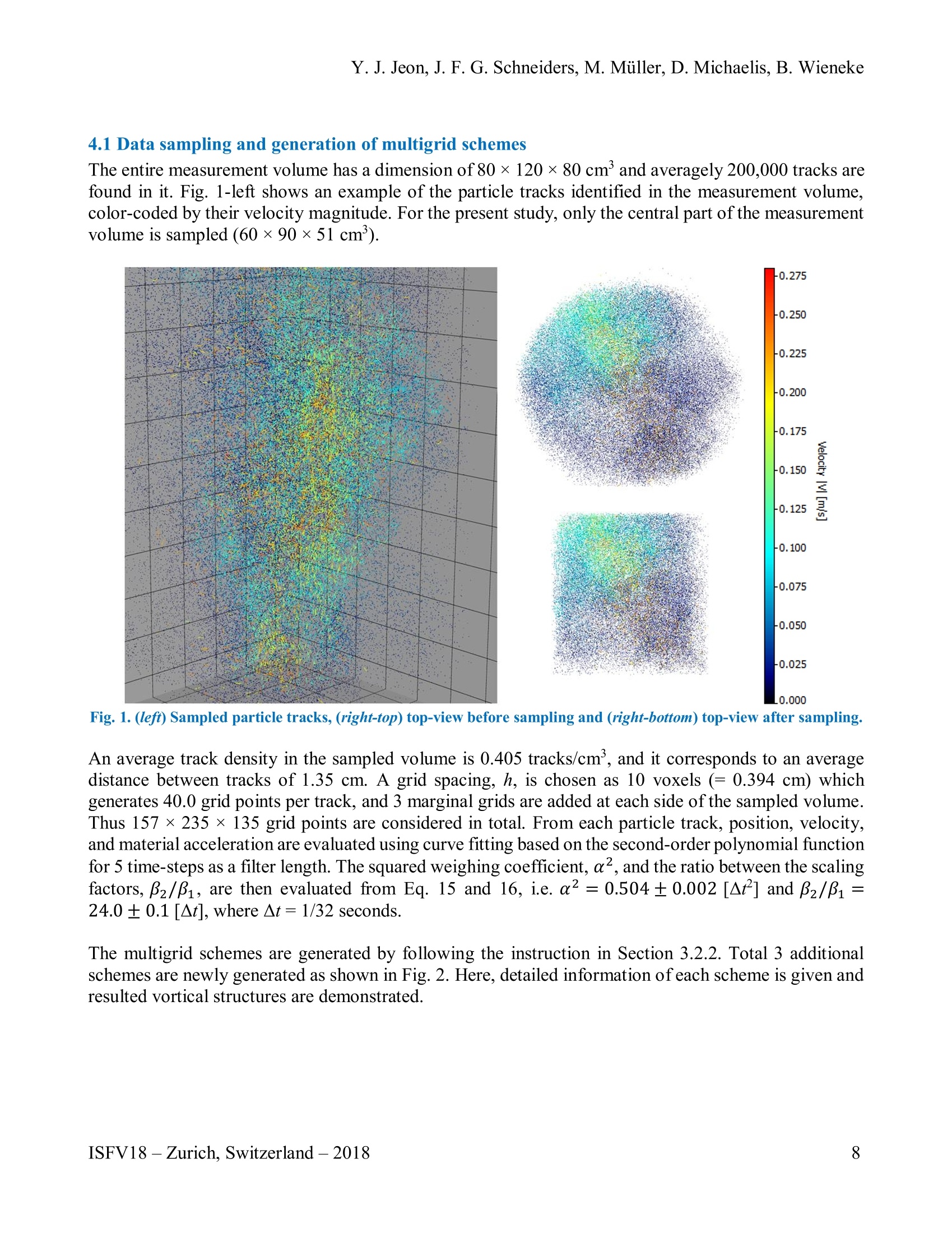
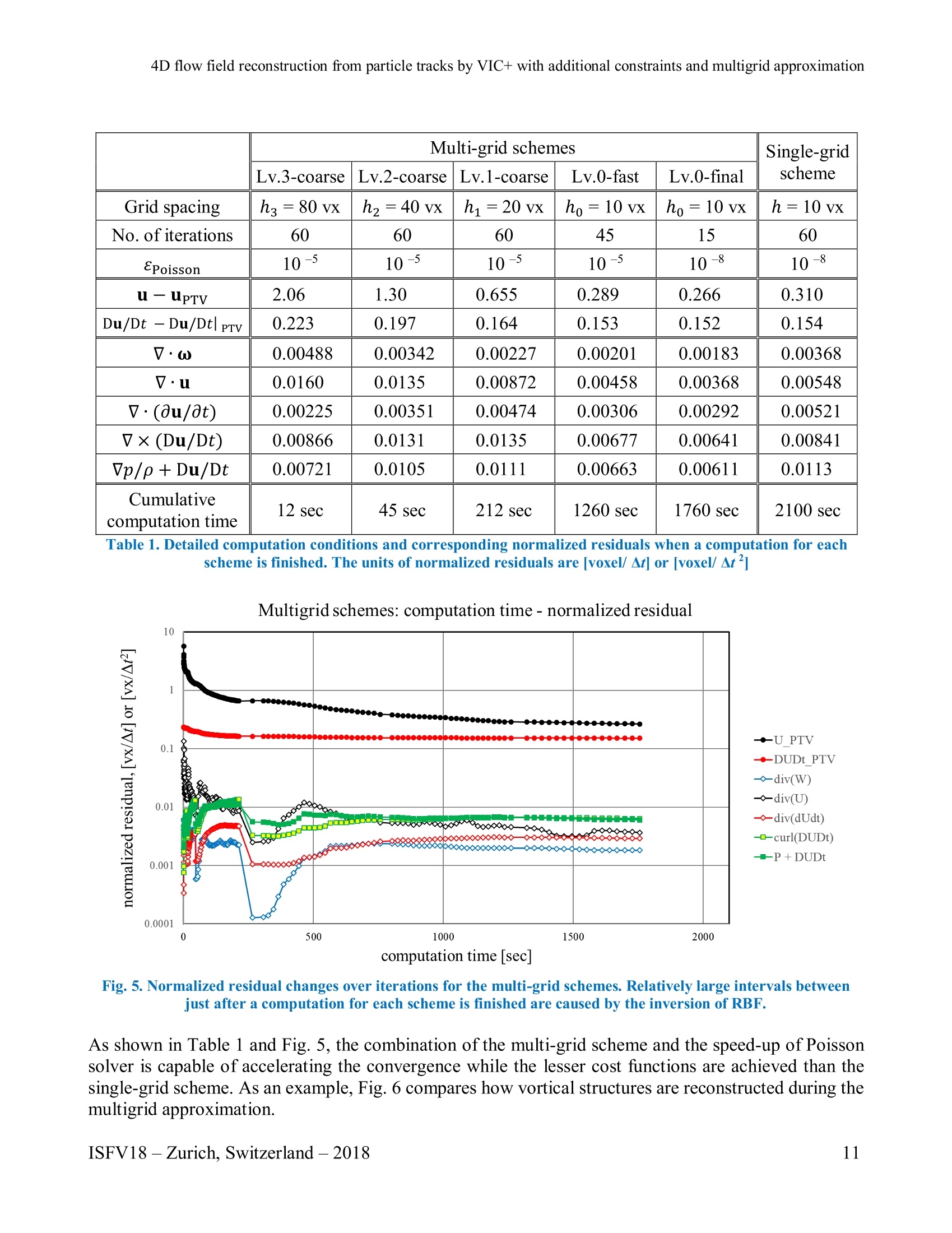
Research Collection 18* International Symposium on Flow VisualizationZurich, Switzerland, June 26-29, 2018 Conference Paper 4D flow field reconstruction from particle tracks by VIC+ withadditional constraints and multigrid approximation Author(s: Jeon, Y.J.; Schneiders, J.F.G.; Muller, M.; Michaelis, D.; Wieneke, B. Publication Date: 2018-10-05 Permanent Link: https://doi.org/10.3929/ethz-b-000279199 Rights /License: In Copyright-Non-CommercialUse Permitted → This page was generated automatically upon download from the ETH Zurich Research Collection. For moreinformation please consult the Terms of use. 4D FLOW FIELD RECONSTRUCTION FROM PARTICLE TRACKS BY VIC+WITH ADDITIONAL CONSTRAINTS AND MULTIGRID APPROXIMATION Y. J. Jeonl,J. F. G. Schneiders,M. Miller, D. Michaelis, B. Wieneke LaVision GmbH, Gottingen, D-37081, Germany "Department of Aerospace Engineering, TU Delft, Delft, 2628 CD, The NetherlandsCorresponding author: Tel.:+49 (0)551 9004-0; Fax: +49 (0)551 9004-100;Email:yjeon@lavision.de KEYWORDS: Main subjects: Numerical techniques in quantitative flow visualization Visualization methods: Shake-the-Box (STB) and Vortex-in-Cell-plus (VIC+) Other keywords: data assimilation, pressure, PTV, multi-grid approximation ABSTRACT: The present work investigates how to enhance Vortex-in-Cell-plus (VIC+) [1], capable ofreconstructing 4D flow fieldfrom dense time-resolved particle track measurement such as Shake-the-Box (STB,4D-PTV) [2, 3]. This study focuses on two aspects: removal of the necessity of initial condition andimprovement of computation speed. For the former, the criteria ofthe parameters, for updating boundarycondition and for weighting time derivatives, are modified to be evaluated from STB without an initial guessof the flow field. In addition, the continuity equation and Navier-Stokes equation from which additionalconstraints to flow field are derived are newly integrated into the cost function ofVIC+ in order to update theboundary condition progressively and reliably. For the computational speed, a concept of the iterative multi-grid approximation [4] is adopted in order both to save the computational resource and to provide moredesirable flow field by cropping out the erroneous computation boundary before triggering a successive VIC+optimization for the finer grid scheme. STB measurement under the densely seeded condition is taken intoaccount and its fluid structures, pressure field, and computational performances are demonstrated. 1 Introduction Shake-the-Box [2, 3] has emerged as novel time-resolved particle tracking velocimetry (4D PTV) that iscapable of achieving accurate and ghostless reconstruction of Lagrangian tracks from densely seededparticle images. Conversion of the Lagrangian tracks to an Eulerian vector field is required for furtheranalyses which are generally conducted on the regular 3D grid. Moreover, recent studies using Vortex-in-Cell-plus (VIC+)[1, 7] and FlowFit [5] have shown increased measurement fidelity and resolution ona regular grid by processing the particle tracks using data assimilation concept, regardless of imbalancedlocal particle concentration. VIC+ and FlowFit iteratively optimize flow field variables including velocity and material accelerationby minimizing their own cost functions using the limited-memory Broyden-Fletcher-Goldfarb-Shanno(L-BFGS) [6]. The principal difference between the two methods is that main variables which are directlytaken into account by L-BFGS are different to each other: VIC+ optimizes a vorticity field and boundaryvalues of velocity and acceleration, whereas FlowFit optimizes a velocity field and a pressure field. Otherfluid variables such as material acceleration and convection terms are derived from these main variablesby invoking the Navier-Stokes equations. In the successive studies [7, 8, 9, 10], it has been shown thatVIC+ and FlowFit are able to provide desirable flow fields. A recent study with VIC+ [7] has demonstrated by application of the technique to real-world turbulentboundary layer measurements that the technique is able to reconstruct dissipation and vorticity, thatwould otherwise be damped by more than 40%. However, the study also highlighted the relativedifficulty of using such a technique, indicating the required computational time and the requirement foran initial condition (that can be obtained from e.g. PIV or a computationally inexpensive particle trackinterpolation scheme). Moreover, the technique uses a range of closure parameters that are scaledautomatically [1], but a study into the optimal settings is still left for future research. The present study focuses on how to efficiently utilize VIC+ and to enhance it for various STBmeasurement conditions. In a practical viewpoint, the most difficult but mandatory preprocessing is toestimate initial velocity field, from which VIC+ is started and by which the weighting coefficients forvelocity and acceleration boundaries are defined, since designing interpolation and extrapolationmethods to deal with various measurement conditions would be another laborious task. The simplest way to avoid this difficulty is that initializing VIC+ from zeros with modified definitionsfor the weighting coefficients irrelevant to the initial condition, and this is what the present studyendeavors. VIC+ initialized from zeros, however, gives rise to another issue that the convergence mightbe halted due to the overcorrection of the boundary conditions, caused by the initially overestimatedweighting coefficient. The present method adds constraints based on the continuity equation and Navier-Stokes equation to VIC+ in order to let the boundary condition satisfied with more physical constraintswhile suppressing the diverging boundary conditions. The additional cost functions are integrated intothe original VIC+ optimization with proper weightings, which are estimated from STB measurement. The second practical issue of VIC+ is the computation time. Although a memory-efficient optimizationis used (L-BFGS [6]), VIC+ requires significant computational time comparable to tomographic PIV.Accordingly, a time-sliding implementation was proposed recently [7] to allow more efficient evaluationof time-sequences. A second improvement is proposed in the present study, inspired from the PIVcommunity, where it is widely accepted that iterative multi-grid schemes [4] are able to rapidly providean approximate solution on a coarse grid that can speed up convergence on consecutive finer grids. Thepresent study applies this concept to VIC+ optimization and investigates its performance in terms ofresiduals and computation time. The present method is tested using an experiment in a thermal plume processed using STB and measuredunder a densely seeded condition [11, 12]. Effectivenesses of the additional constraints and the multigridapproximation are shown as residual changes during the optimization. Highly populated flow structuresare reconstructed and their growth, movement, and interaction with each other are clearly visualized.Time-resolved pressure fields which correspond to the flow structures are evaluated as well. Prior to describing the present method, the authors briefly review VIC+. Then new features and modifiedones follow after this section. An optimization variable of VIC+,, which is optimized by the L-BFGS algorithm, consists of t, an,uand tan,0u/ot, Here, Bi and B2 are scaling factors to consider different physical units in order to optimze each elementoft with evenly distributed residuals, and these are derived from standard deviations o of tag,u andtan,ou as following. A vorticity field, ω, a velocity boundary, uan, and an acceleration boundary,Ou/otan, are derived from5a, tan,uand tan,du/at respectively by means of the Gaussian radial basis function (RBF),d: and h is the grid spacing. A velocity field and an acceleration field are then obtained by respectivelysolving the following Poisson equations with Dirichlet boundary conditions given by Eq. 4 and Eq. 5: Here the vorticity time derivative field is derived from the vorticity transport equation. A material acceleration, Du/Dt, is defined on the grid by, The cost function to which the L-BFGS refers during its iterative optimization is defined by, ISFV18 -Zurich, Switzerland-2018 Here a is the weighing coefficient defined by standard deviations of the PTV velocity and materialacceleration measurements. For the L-BFGS optimization, adjoint functions for Eq.3-5 and Eq.7-10 should be defined. Then the L-BFGS algorithm iteratively searches for the best gradient vector of the optimization variable, , andupdates. A convergence criterion is given as following based on the initial value of the cost function Jo. The original evaluation of a, Eq.13, greatly depends on the magnitude of velocity and materialacceleration. As an iterative optimization is conducted, however, a contribution of the materialacceleration surpasses that of the velocity due to the generally overestimated a. In order to overcomethis, the present method defines a by additionally evaluating a higher order polynomial trajectory. Whenthe velocity, u, and material acceleration, Du/Dt, are estimated from the n-th order polynomial,additional velocity and acceleration are estimated from the (n+1)-th or (n +2)-th order polynomial,i.e. uHo and Du/Dt Ho. The modified definition of a used in the present method is then When the higher polynomial order is not available due to not enough time-steps, a selection of a"between 0.1At and 1.0At is suggested, where At is the time interval between successive snapshots. 3.1.2 Scaling factors, pi and pz As mentioned, the purpose of the scaling factors is to consider different physical units, i.e. vorticity,velocity, and acceleration. The original definitions of Bi and B2, Eq. 2, are based on the real values ofeach component. In the present study, VIC+optimization starts from zeros and it is impossible to givethe scaling factors in advance. In addition, there is a possibility that the boundary values of velocity andacceleration can be so small or so large that the scaling factors and a following optimization are spoiled.This would be further detailed in the Section 3.2.1. The present study defines the scaling factors based on the grid spacing h and the magnitude ratio ofPTVvelocity to PTV acceleration, For Bi, the term of 2h is introduced to consider that vorticity could be derived from velocity based oncentral difference scheme. For B2, the magnitude ratio between the standard deviations, is used as amultiplier. 3.1.3 Interpolation scheme For evaluating fractional velocity and material acceleration from the grid scheme, the tri-cubicinterpolation scheme is used instead of the tri-linear interpolation of the original VIC+, where a =-0.5 is selected. 3.2 New features, added to VIC+ 3.2.1 Additional constraints Ifthe boundary conditions, uan and du/ot|an, are perfect, solving Eq. 7 and Eq. 8 are able to guaranteethe divergences of velocity, V.u, and acceleration, V·(0u/0t), are negligibly small. Although theboundary conditions are corrected during VIC+optimization, its stability ofconvergence greatly dependson the scaling factors, Bi and B2. In addition, it is important to balance between the stability ofconvergence and the convergence speed. As described in the Section 3.1.2, the scaling factors are defined from PTV measurement and thus smallenough to progressively update the boundaries. However, the convergence is no longer stable with thesevalues. In order to assure the stable convergence, the present study takes into account the continuityequation and Navier-Stokes equations from which five additional constraints are derived. Correspondingcost functions are expressed as follows: ISFV18 - Zurich, Switzerland-2018 Note that the viscosity term is neglected in Eq. 21 and Eq. 22 as well as the vorticity transport equation,Eq. 9. Here, the field of pressure divided by density,p/p, is reconstructed by solving a Poisson equation, For solving the above equation, Neumann boundary conditions are imposed to all boundary except oneDirichlet boundary condition with an arbitrary constant value to avoid the singularity. After solving thePoisson equation, the field of p/p is uniformly adjusted to make its averaged value as zero. The new cost function is then defined by, Here the constant value of 8 is chosen to maintain evenly distributed residuals between one particle trackand 8 grid points. 3.2.2 Multi-grid approximation The computation time of VIC+ is significant when a high spatial resolution is required, e.g. a half gridspacing yields 8 times more grid nodes and consequently 8 times of the computation time. In order tosave the computation time, the present study adopts the iterative multigrid approach [10] which arewidely accepted and used in PIV society. The multi-grid approximation with a doubled grid spacing, 2h,takes into account about 1/8 grid points of the final grid scheme, and thus less computation time isrequired. The coarse grid schemes and their number are defined by the following sequence. Step 1. Set the grid spacing, hk, for the coarse grid scheme, k: Step 2. Set the first grid points of k,2x(0,0,0), as: Step 3. Add additional grid points while k covers all the finer grid points of k-1 Step 4. Count width, height, and depth of grids of ki.e. Xk, Ye and Zk. Step 5. If Xk<-Xk-1 or Yk<-Yx-1 or Zk <-Zk-1, go to Step 1, or abandon 2k and the numberofthe grid schemes including the final, 2o, is k. As the result, the finer grid points always fractionally positioned at 0.25 or 0.75 of the coarse grid. Whenmoving on from the coarse grid to the finer grid, it is required to interpolate the optimization variables,. However, because it is laborious to consider the edge and corner effect which are already embeddedin the RBFs in Eq. 2-4, the present study deals with physical variables instead. Firstly, velocity andacceleration vectors in finer grid points are interpolated from the coarser grid points by means of the tri-cubic interpolation, and then a vorticity vector field is evaluated from the velocity vector field, Lastly, optimization variables, a, tan,u and tan,u/ot, are reconstructed by taking the inverse of RBFsexpressed in Eq. 2-4 by means ofthe conjugate gradient method. 3.2.3 Speed-up of Poisson solver for coarse grid schemes In VIC+ optimization, 12 Poisson equations should be solved at each L-BFGS iteration, i. e. Eq.7, 8, andtheir adjoints with three components. Therefore, a computation time for the Poisson equations is anotherissue, and it occupies approximately a half of the total computation time of VIC+. In the present method,the Poisson equations are solved using the algebraic multigrid method [13] with the conjugate gradientmethod. In the conjugate gradient method, it is possible to stop its iteration if a large tolerance can beaccepted. In the present study, the multi-grid approximation and 3/4 of iterations for the final grid schemeuse the large tolerance, Epoisson =10-5, and the remained iterations for the final grid scheme isconducted with a smaller tolerance, Epoisson=10-8. Note that the large tolerance, Epoisson = 10-5,could be achieved by about 30% ofa computation time to achieve the small tolerance, Epoisson =10-8. 4 Results The present method is in the case of the measurement of a pure thermal plume at cubic meter scales bycourtesy of German Aerospace Center (DLR, Gottingen, [11,12]). To achieve the large measurementvolume, helium-filled soap bubbles (HFSB) are used as tracer particles. The measurement data areprocessed by STB to yield particle trajectories. All the data processing methods mentioned in this study,i.e. STB, VIC+, and the present method, are conducted using DaVis 10 software. The entire measurement volume has a dimension of 80×120×80 cm’and averagely 200,000 tracks arefound in it. Fig. 1-left shows an example of the particle tracks identified in the measurement volume,color-coded by their velocity magnitude. For the present study, only the central part of the measurementvolume is sampled (60×90×51 cm’). Fig. 1. (left) Sampled particle tracks, (right-top) top-view before sampling and (right-bottom) top-view after sampling. An average track density in the sampled volume is 0.405 tracks/cm’, and it corresponds to an averagedistance between tracks of 1.35 cm. A grid spacing, h, is chosen as 10 voxels (= 0.394 cm) whichgenerates 40.0 grid points per track, and 3 marginal grids are added at each side of the sampled volume.Thus 157×235 ×135 grid points are considered in total. From each particle track, position, velocity,and material acceleration are evaluated using curve fitting based on the second-order polynomial functionfor 5 time-steps as a filter length. The squared weighing coefficient, a2, and the ratio between the scalingfactors, B2/Bi, are then evaluated from Eq. 15 and 16,i.e. a²=0.504±0.002[^t] and B2/B1=24.0±0.1[At], where t=1/32 seconds. The multigrid schemes are generated by following the instruction in Section 3.2.2. Total 3 additionalschemes are newly generated as shown in Fig. 2. Here, detailed information of each scheme is given andresulted vortical structures are demonstrated. (a) multigrid level=3 (b) multigrid level=2 (c) multigrid level=1 (d) final grid Fig.2. Example of multigrid generation: vortical structures are visualized as iso-surfaces of 12. Note that criteria forthe iso-surfaces are differ. 4.2 Additional constraints to VIC+ To investigate whether the additional constraints are helpful when no favorable initial condition isavailable, the cost functions from Eq. 18-22 are obtained after each iteration. The cost functions arenormalized to have dimensions identical to the units of velocity or acceleration, i.e. [voxel/At] or[voxel/At'] respectively. Note that only the final grid scheme with 60 iterations is considered. Fig. 3compares the residual changes over 60 iterations for both cases. present method without the additional constraints present method with the additional constraints Fig. 3. Comparison of the normalized residual changes over iterations without an initial guess of flow field: (left)present method without the additional constraints, (right) present method with the additional constraints. Fig. 3-left shows that when the additional constraints are not considered for the optimization, theirresidual values based on the physical constraints can increase with an increasing number of iterations.Instead, the velocity and material derivative constraints are penalized in the optimization and reduce withevery iteration. Fig. 3-right shows that when the additional constraints are included, recalling eq. 24: their values eventually reduce instead of increasing the number of iterations. This indicates enhancedstability of the optimization procedure, as these physical constraints remain satisfied, even when a largenumber of iterations is considered. Fig. 4 supplements that the present method’s modified weightingcoefficients, α, and scaling factors, Bi and B2, are not able to guarantee a stable convergence without theadditional constraints due to the diverging boundaries. X [mmm] X[mm] Fig. 4. Comparison of velocity divergences, the x-y plane at the middle of z-direction, the vectors denote velocityfields and its divergences are shown as the scalar fields: (left) the present method without the additional constraints,(right) the present method with the additional constraints.The marginal grids are included. 4.3 Multi-grid approximation An effectiveness of the multi-grid approximation is tested by collecting residuals at each iteration. 60iterations are conducted per each scheme and the speed-up ofthe Poisson solver with the relaxed residualis also applied. In Table 1, the detailed computation conditions for each level are listed and correspondingresiduals from each cost function are compared to the single grid scheme. In addition, Fig. 5 shows theresidual changes over 240 iterations in total including the multigrid approximation schemes and the finalgrid scheme. Multi-grid schemes Single-gridscheme Lv.3-coarse Lv.2-coarse Lv.1-coarse Lv.0-fast Lv.0-final Grid spacing h3=80 vx h2=40 vx h1=20vx ho=10 vx ho= 10 vx h=10 vx No. of iterations 60 60 60 45 15 60 cPoisson 105 10-5 10-5 10-5 10-8 10-8 u-upTv 2.06 1.30 0.655 0.289 0.266 0.310 Du/Dt -Du/Dt|PTy 0.223 0.197 0.164 0.153 0.152 0.154 V·0 0.00488 0.00342 0.00227 0.00201 0.00183 0.00368 V·u 0.0160 0.0135 0.00872 0.00458 0.00368 0.00548 V· (0u/0t) 0.00225 0.00351 0.00474 0.00306 0.00292 0.00521 V× (Du/Dt) 0.00866 0.0131 0.0135 0.00677 0.00641 0.00841 Vp/p +Du/Dt 0.00721 0.0105 0.0111 0.00663 0.00611 0.0113 Cumulative computation time 12 sec 45 sec 212 sec 1260 sec 1760 sec 2100 sec Table 1. Detailed computation conditions and corresponding normalized residuals when a computation for eachscheme is finished. The units of normalized residuals are [voxel/ Ator [voxel/ At] Multigrid schemes: computation time- normalized residual Fig. 5.Normalized residual changes over iterations for the multi-grid schemes. Relatively large intervals betweenjust after a computation for each scheme is finished are caused by the inversion of RBF. As shown in Table 1 and Fig. 5, the combination of the multi-grid scheme and the speed-up of Poissonsolver is capable of accelerating the convergence while the lesser cost functions are achieved than thesingle-grid scheme. As an example, Fig. 6 compares how vortical structures are reconstructed during themultigrid approximation. Fig. 6. Evolution of vortical structures during multigrid approximation. Even though there are small differences between two cases, the overall qualities of reconstruction at thefinal scheme seem similar. Therefore, only 40 iterations are used per each scheme for the followingresults. 4.4 Time-resolved reconstruction, 4D flow field Fig. 7 demonstrates how flow structures are driven by the inner flow. The inner flow core caused bybuoyancy leans to the right-backward side and its interaction with relatively stable surrounding flowgenerates numerous turbulent vortical structures. Corresponding low-pressure structures are also visiblein where the vorticial structures are clustered together. The high-velocity region at middle height,detached between t=0 and 1, and corresponding low-pressure structures are identified. This low-pressurestructure seems to be decelerated because it recedes from the flow core while its size expands. Fig. 7. Instantaneous snapshots for velocity, vortical structures, and pressure.Color-coded iso-surfaces indicatevelocity magnitude, from 0.0 m/s to 0.23 m/s. A single grid in the background indicates 0.1 m. 5 Conclusion The present work has focused on the efficient and stable implementation of VIC+ in a commercialsoftware package (Davis 10). The most significant difficulty of the implementation is a necessity of theinitial guess of flow field which is for not only initial condition of the optimizer but also the importantfactors. The present method modifies the criteria for the weighting coefficient and the scaling factors aremodified to be evaluated from PTV measurement. And thus, VIC+ is now able to reconstruct a flow fieldfrom zeros without any initial condition given. The original VIC+ takes into account Navier-Stokesequation as the vorticity transport equation. In addition to that, the present method directly takes intoaccount Navier-Stokes equation and the continuity equation. As the results, the stable convergence canbe guaranteed with the small scaling factors which cause large changes in the boundary condition. Multi-grid approximation, inspired by multi-grid PIV, and the speed-up of Poisson solver are tested inorder to save the massive computation time of VIC+ and successfully implemented in VIC+. The savingrate oftheir combination is estimated up to 40% ofthe original computation time. Time-resolved pressurefields are also considered and thus available during the optimization procedure of VIC+. ( [1] Schneiders J FG a n d Scarano F. Dense vel o city reconstruction fr o m tomographic PTV with m aterial deriv a tives.Experiments in Fluids, V ol.5 7 , No.9, pp.139, 2016 ) [2] Schanz D, Schroder A, Gesemann S, Michaelis D and Wieneke B, Shake The Box: A highly efficient and accuratetomographic particle tracking velocimetry method using prediction of particle positions, 10th Int. Symp. on particle imagevelocimetry -PIV13,Delft, The Netherlands, 2013 ( [3]S S chanz D , Gesemann S a n d Schroder A, S hake-The-Box: Lag r angian particle tr a cking at high p a rticle i magedensities. Experiments in Fluids, Vol. 57 No.5,p p .70, 2 0 16 ) ( [4]S S carano F. and Riethmuller ML, Advances in it e rative multigrid PIV i m age processing. Experiments in Fluids, Vol.29,No.1, pp.S051-S060,2000 ) ( [5] G esemann S, Huhn F, Schanz D, Schro d er A. From n o isy p a rticl e tracks to veloci t y, acceleration and p r essure fieldsusing B -splines and penalties. In: 18th international symposium on a pplications oflaser and imaging techniques to fluidmechanics, L i sbon, P o rtugal, 2016 ) ( [6] N ocedal J. Updating quasi-Newton matrices with limited storage.Mathematics ofcomputation, Vol. 3 5,No.151 , pp.773-82,1980 ) ( [7] Schneiders J FG, S carano F , and E l singa GE. R e solving vorticity and dissipation in a turbulent boundary layer by t omographic PTV a n d VIC+. Experiments in F l uids, V ol.58, No.4, pp.27, 2017 ) ( 8]S S chneiders JFG, Avallone F , Probsting S, R agni D, and Scarano F . Pressure spectra from s ingle-snapshot tomographicPIV. E xperiments in Fluids, Vol.59, N o.3, p p.57, 201 1 8 9 ) ( [9]I H uhn F , Schanz D , Gesemann S, Dierksheide U, van de Meerendonk R, a nd Schroder A. Large-scale vo l umetric flowmeasurement in a pure th e rmal plume by dens e tracking of helium-filled soap bubbl e s. Experiments in Fluids, Vol. 58 , No.9,pp.116,2017 ) ( [ 1 0]Schanz D, Schroder A, Gesemann S, Huhn F, Novara M, Geisler R , Manovski P , Depuru-Mohan K. R e cent A d vances inVolumetric F low Measurements: High-Density Pa r ticle T r acking ( ‘ Shake-The-Box’) with Navier-Stokes RegularizedInterpolation (FlowFit’). New Results in Numerical and Experimental Fluid Mechanics XI, pp. 587-597. Springer,Cham,2018 ) ( [11 ] Schanz D, H uhn F , Gesemann S, D ierksheide U, van de Meerendonk R, Manovski P, and S chr o der A. T o wa r ds high-resolution 3D flow field measurements at cubic meter scales. In: 18th international symposium on app l ications oflasertechniques to fluid mechanics, L i sbon, Portugal, 2016 ) [12]Huhn F, Schanz D, Gesemann S, Dierksheide U, van de Meerendonk R, and Schroder A. Large-scale volumetric flowmeasurement in a pure thermal plume by dense tracking of helium-filled soap bubbles. Experiments in Fluids, Vol.58,No.9, pp.116,2017 [13]Stiiben K, An introduction to algebraic multigrid. Multigrid,pp.413-532, 2001 Copyright Statement The authors confirm that they, and/or their company or institution, hold copyright on all the original material included in theirpaper. They also confirm they have obtained permission, from the copyright holder of any third-party material included intheir paper, to publish it as part of their paper. The authors grant full permission for the publication and distribution of theirpaper as part of the ISFV18 proceedings or as individual off-prints from the proceedings. ETHLibrarv ISFV- Zurich, Switzerland- The present work investigates how to enhance Vortex-in-Cell-plus (VIC+) [1], capable ofreconstructing 4D flow field from dense time-resolved particle track measurement such as Shake-the-Box (STB,4D-PTV) [2, 3]. This study focuses on two aspects: removal of the necessity of initial condition and improvement of computation speed. For the former, the criteria of the parameters, for updating boundary condition and for weighting time derivatives, are modified to be evaluated from STB without an initial guess of the flow field. In addition, the continuity equation and Navier-Stokes equation from which additional constraints to flow field are derived are newly integrated into the cost function of VIC+ in order to update theboundary condition progressively and reliably. For the computational speed, a concept of the iterative multigrid approximation [4] is adopted in order both to save the computational resource and to provide more desirable flow field by cropping out the erroneous computation boundary before triggering a successive VIC+ optimization for the finer grid scheme. STB measurement under the densely seeded condition is taken into account and its fluid structures, pressure field, and computational performances are demonstrated.
确定


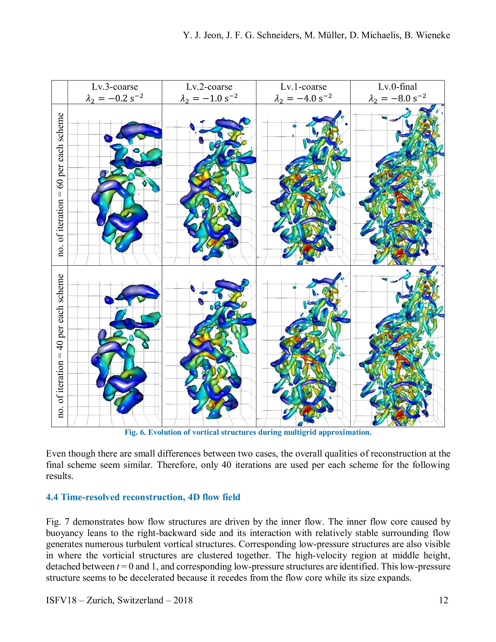
还剩14页未读,是否继续阅读?

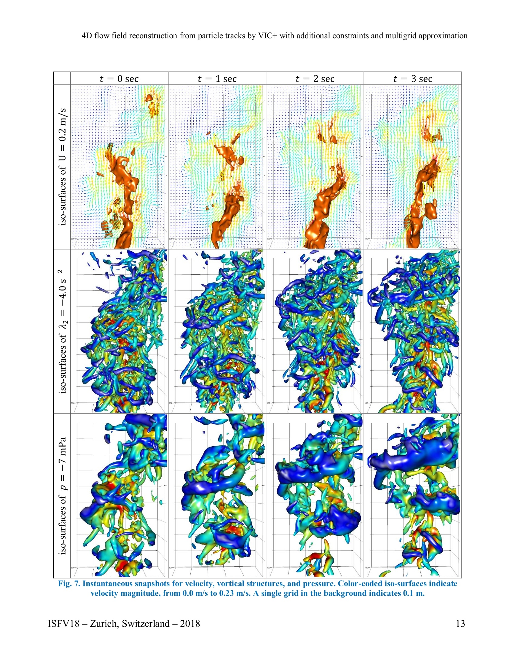
产品配置单


北京欧兰科技发展有限公司为您提供《流动对象中4D流场检测方案(粒子图像测速)》,该方案主要用于其他中4D流场检测,参考标准--,《流动对象中4D流场检测方案(粒子图像测速)》用到的仪器有体视层析粒子成像测速系统(Tomo-PIV)、LaVision DaVis 智能成像软件平台
推荐专场


相关方案
更多
该厂商其他方案
更多