流场中3D3C速度矢量场检测方案(粒子图像测速)

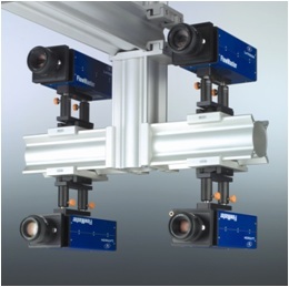
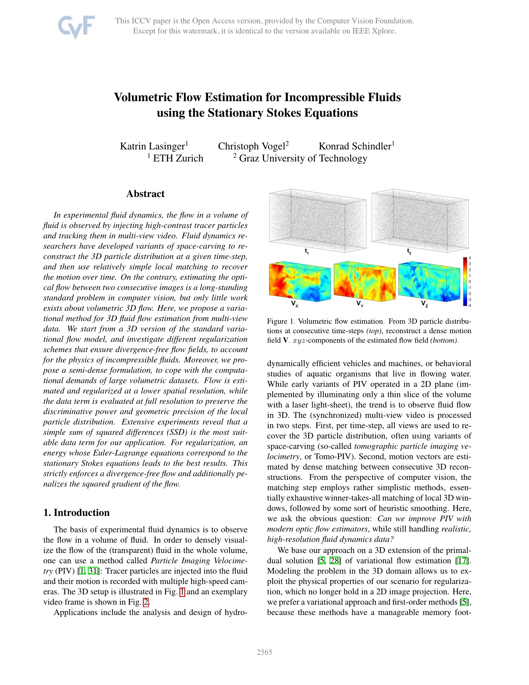
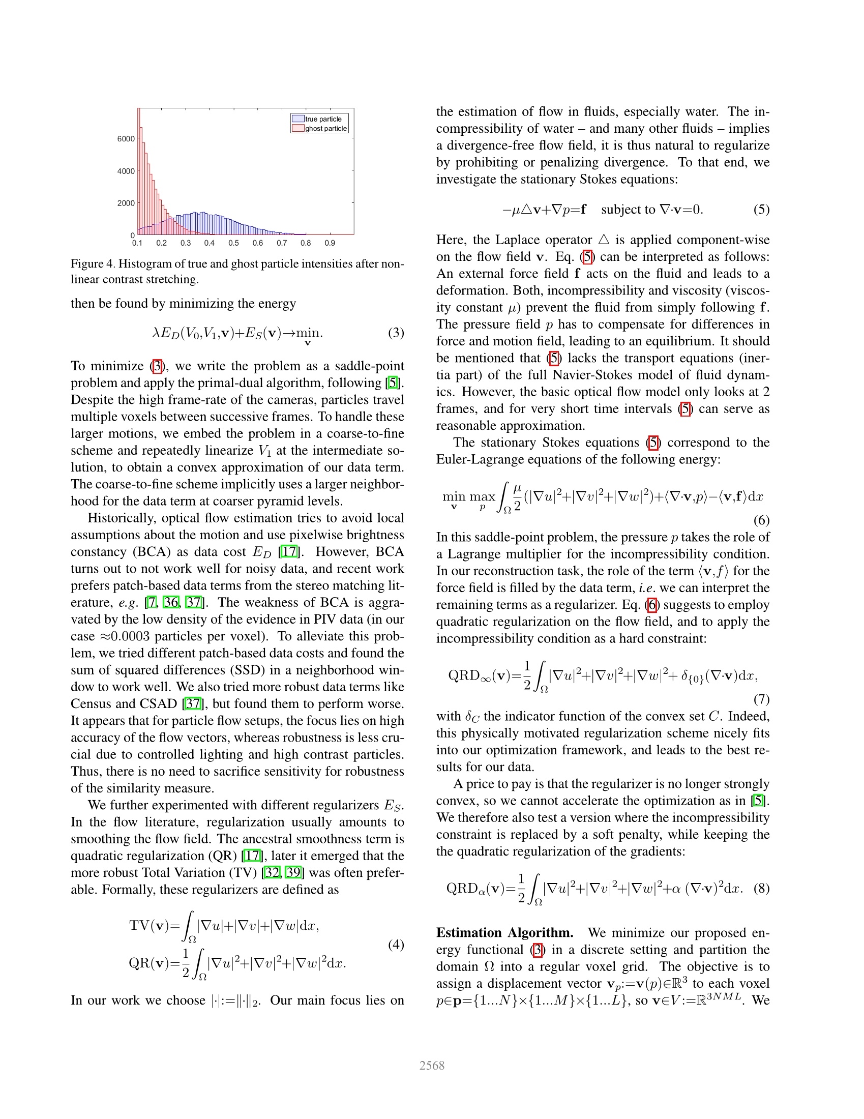
This ICCV paper is the Open Access version， provided by the Computer Vision Foundation.Except for this watermark， it is identical to the version available on IEEE Xplore. Volumetric Flow Estimation for Incompressible Fluidsusing the Stationary Stokes Equations Katrin Lasinger Christoph Vogel Konrad Schindler ETH Zurich Graz University of Technology In experimental fluid dynamics， the flow in a volume offluid is observed by injecting high-contrast tracer particlesand tracking them in multi-view video. Fluid dynamics re-searchers have developed variants of space-carving to re-construct the 3D particle distribution at a given time-step，and then use relatively simple local matching to recoverthe motion over time. On the contrary， estimating the opti-cal flow between two consecutive images is a long-standingstandard problem in computer vision， but only little workexists about volumetric 3D flow. Here， we propose a varia-tional method for 3D fluid flow estimation from multi-viewdata.We start from a 3D version of the standard varia-tional fow model， and investigate different regularizationschemes that ensure divergence-free flow fields， to accountfor the physics of incompressible fluids. Moreover， we pro-pose a semi-dense formulation， to cope with the computa-tional demands of large volumetric datasets. Flow is esti-mated and regularized at a lower spatial resolution， whilethe data term is evaluated at full resolution to preserve thediscriminative power and geometric precision of the localparticle distribution. Extensive experiments reveal that asimple sum of squared differences (SSD) is the most suit-able data term for our application. For regularization， anenergy whose Euler-Lagrange equations correspond to thestationary Stokes equations leads to the best results. Thisstrictly enforces a divergence-free flow and additionally pe-nalizes the squared gradient of the flow. 1. Introduction The basis of experimental fluid dynamics is to observethe flow in a volume of fluid. In order to densely visual-ize the flow of the (transparent) fluid in the whole volume，one can use a method called Particle Imaging Velocime-try (PIV) @31]： Tracer particles are injected into the fluidand their motion is recorded with multiple high-speed cam-eras. The 3D setup is illustrated in Fig.；.and an exemplaryvideo frame is shown in Fig.2 Applications include the analysis and design of hydro- Figure 1. Volumetric flow estimation. From 3D particle distribu-tions at consecutive time-steps (top)， reconstruct a dense motionfield V. cyz-components of the estimated flow field (bottom). dynamically efficient vehicles and machines， or behavioralstudies of aquatic organisms that live in flowing water.While early variants of PIV operated in a 2D plane (im-plemented by illuminating only a thin slice of the volumewith a laser light-sheet)， the trend is to observe fluid flowin 3D. The (synchronized) multi-view video is processedin two steps. First， per time-step， all views are used to re-cover the 3D particle distribution， often using variants ofspace-carving (so-called tomographic particle imaging ve-locimetry， or Tomo-PIV). Second， motion vectors are esti-mated by dense matching between consecutive 3D recon-structions. From the perspective of computer vision， thematching step employs rather simplistic methods， essen-tially exhaustive winner-takes-all matching of local 3D win-dows， followed by some sort of heuristic smoothing. Here，we ask the obvious question： Can we improve PIV withmodern optic flow estimators， while still handling realistic，high-resolution fluid dynamics data? We base our approach on a 3D extension of the primal-dual solution 28] of variational flow estimation [[Z].Modeling the problem in the 3D domain allows us to ex-ploit the physical properties of our scenario for regulariza-tion， which no longer hold in a 2D image projection. Here，we prefer a variational approach and first-order methods [5]，because these methods have a manageable memory foot- Figure 2. Particle image from one view， with zoomed detail. print and offer the possibility to include the aforementionedphysical constraints. As in the 2D case， @36， 37]， weprefer to use window-based data terms rather than per-pixelbrightness constancy. For our (soft， probabilistic) particlevolumes， where all particles look the same， we posit thatmatching information can still be found in the local patternsof the particles. Standard regularizers， like a quadratic penalty on the thegradients of the flow field or total variation (TV)， do notconsider the special properties ofliquids， which are incom-pressible and thus should have a divergence-free flow field.Regularizers which penalize divergence have been tried forboth 2D and 3D problems 2. 13.14. Here， we proposean energy whose optimality conditions correspond to thestationary Stokes equations. This energy formulation inte-grates nicely into our optimization framework and leads tothe desired incompressibility constraint on the flow field. A challenge of 3D flow estimation is the high compu-tational cost， as the number of voxels， respectively vari-ables， increases cubically with the resolution. On one hand，one could argue that lower-resolution reconstruction is suf-ficient， because the effective resolution of PIV is limited bythe particles’size and density. On the other hand， naivelydown-sampling the volume will drastically smooth out thelocal particle likelihood， and thereby destroy both robust-ness against mismatches and localization accuracy.Wetherefore propose a semi-dense approach， where flow vec-tors are computed (and regularized) on a lower-resolutiongrid， while the data-term is evaluated at full resolution toretain the precision and robustness ofthe original particledistribution. We demonstrate that the results of the semi-dense approach are comparable to per-voxel flow estima-tion， but able to handle large volumetric datasets recordedwith modern high-resolution sensors. In our experiments，the proposed method is superior to simple local flow es-timation and， without any post-processing， delivers resultscomparable with the best available3D fluid flow methods. 2. Related Work In experimental fluid mechanics， particle imaging ve-locimetry (PIV) is the estimation of a dense velocity fieldin a fluid volume with the help of tracer particles and op-tical images 31. Though traditionally focusing on 2D motion on a single laser sheet， recent PIV approaches alsotackle 3D velocity fields33]. Elsinga et al.111werethe first to handle high particle densities in 3D with their to-mographic particle image velocimetry (Tomo-PIV) method.Per time-step， the particle distribution in the volume of in-terest is reconstructed from multi-view imagery. The veloc-ity field is estimated by subsequent 3D cross-correlation oflarge local 3D windows (in PIV terminology “interrogationvolumes") containing the reconstructed particles. The largesize of the interrogation volumes， determined by the practi-cally viable particle density， limits the spatial resolution ofthe reconstructed flow field. More recent methods have fo-cused on post-processing multiple consecutive two-view ve-locity fields with the help of a dynamic model to increase re-construction quality [25]. Technical approaches include it-erative volume deformation with adaptive window sizes [⑧]，methods in the spirit of Lucas-Kanade tracking [夕] and re-constructing trajectories of pa11rticle patterns over time [21].Schanz et al. [33] propose tracking of individual particlesover long time sequences instead. While tracking individ-ual particles is certainly an option to refine PIV results， thebasic two-frame case is arguably better captured by denseflow estimation，which more naturally matches the continu-ous and physically constrained nature of flowing fluids. Fur-thermore， individual particle tracking recovers the flow onlyat particle locations. Hence， additional post-processing isneeded to interpolate sparse tracks to a grid and to applythe relevant physical constraints [[12.34]. Heitz et al. [[4]point out potential research directions for variational PIVand advocate the use of correct physical constraints， focus-ing mainly on 2D problems. Alvarez et al.[2] were， toour knowledge， the first to present a variational model of3D-PIV that accounts for the physical properties of incom-pressible fluids. However， their method is applicable onlyas refinement after an initial flow estimation with another(not physically grounded) model. Even so， results are onlyshown for small toy volumes (up to 256×128×144 voxels). Also related is work by Gregson et al. [13]， who pro-pose a flow reconstruction algorithm for dye-injected two-media fluids， primarily aiming for visually pleasing resultsover small volumes (~100 voxels). Their data containsmore structural information than our particle images， hencethe step from 2D to 3D is less ambiguous. On the otherhand， spatial information is available only in areas wheredye is visible， thus multiple time steps are needed to denselycover the domain. Technically， they show that the pressure-projection step， commonly used for fluid simulations， isequivalent to a projection on the divergence-free subspace，which they formulate as a proximal operator. Like theirs，our scheme is also motivated by physical properties of flu-ids， additionally we show that our regularizer emerges froma proper energy formulation， naturally derived from thestationary Stokes equations. It is therefore not necessary， to perform the -computationally expensive - reprojectiononto the subspace of divergence-free motion fields in eachiteration of the algorithm. Instead， we can include incom-pressibility as a hard constraint. With modern optimizationtechniques， this leads to a much more efficient algorithm. In the field of medical image processing， volumetric flowestimation is used to register 3D scans from different imag-ing modalities， e.g.， computer tomography (CT) and mag-netic resonance imaging (MRI). In medical imaging， 3Dflow estimation [623.26.29] is further important for ap-plications that aim to compensate 3D organ motion in time-resolved medical image sequences (e.g.， due to respiration). Recently， 2D optical flow benchmarks have been dom-inated by label-based methods 24]， propagation meth-ods 4i8]， neural regression networks [o] and modelsthat exploit scene-specific properties like semantics [353].Most of these models do not scale well to the volumetric do-main and struggle heavily with memory consumption. Fur-ther， it is not obvious how to incorporate physical proper-ties of the problem into any of them. Finally， our particledata does not provide any semantic， structural or texturalcues. Consequently， we feel that a variational approach isthe most suitable one for our application scenario. 3. Approach Our 3D flow estimation pipeline from multiple perspec-tive images is depicted in Figure3Starting from ≥3 syn-chronous images of the volume， seeded with tracer parti-cles， we perform a 3D reconstruction with our own imple-mentation of the tomographic reconstruction technique -essentially a soft version of space-carving， which outputsa 3D voxel space of “particle presence probabilities”， seeSec. 3.1Two such 3D volumes from consecutive time-steps then serve as input for 3D flow estimation. We preferto work with floating-point scores that indicate the proba-bility of a voxel being occupied， rather than take hard deci-sions about the presence or absence of particles. Our maincontribution， the volumetric flow estimation， is described inSection 3.2. We review the primal-dual approach， introducedata terms， regularizers and complete cost functions for the3D fluid case， and explain the semi-dense flow estimation. Figure 3. Flow estimation pipeline. (left) 2D input data， (middle)3D reconstruction， (right) 3D flow estimation from 2 time steps. 3.1. Tomographic Reconstruction For 3D reconstruction we follow the Tomo-PIV ap-proach and implement the MART algorithm []. Addi- tionally， after each MART iteration we apply anisotropicGaussian smoothing (3×3×1 voxels) to the reconstructedvolume， to account for elongated particle reconstructionsalong the z-axis due to the camera setup . MART is aniterative solver for the inverse problem where I(ci，Vi) denotes the observed pixel intensities，E(X，，Y，Zj) the unknown voxel intensities and R， is alist of all voxels traversed by the viewing ray through pixel(aiyi). The weight wi，E[0，1] depends on the distance be-tween the voxel center and the line of sight and is essentiallyequivalent to an uncertainty cone around the viewing ray， toaccount for aliasing of discrete voxels. For each pixel i inevery camera， and for each voxel j， the following updatestep is performed： The result of the 3D reconstruction is a NxMxL voxelspace with a scalar intensity value per voxel， where highintensity indicates high likelihood that the voxel is occu-pied by a particle. With increasing number/density of par-ticles the ambiguity increases， since multiple 3D configu-rations are plausible that would reproject to the given im-ages. These ambiguities lead to so-called “ghost parti-cles”[22]， which cannot be ruled out with the available ev-idence. Therefore， our flow estimation algorithm will haveto deal with particles that do not actually exist. Ghost par-ticles are on average lower in intensity than true particles.However， the imaging setup also leads to intensity varia-tions between true particles， such that ghost particles can-not be filtered by thresholding. We prefer not to heuristi-cally resolve ambiguities at an early stage， and instead usethe soft， noisy occupancy probabilities as input for 3D flowestimation. MART tends to decrease also the probabilities of trueparticles， see Figure 4.We found it advantageous to applynon-linear contrast stretching to the volume before the sub-sequent flow computation： Eout=(Ein)Y， with y=0.7. 3.2. Volumetric Flow Given two 3D volumes Vo，V：Q→R+， defined over thevolumetric domain 2cR， we aim to reconstruct the 3Dmotion field v：-R3. The functional v=(u，u，w) repre-sents a mapping of points p in Vo to points (p+v) in V. Like 2D optical flow， the problem is ill-posed when rely-ing only on the local similarity Ep(Vo，Vi，v). The solutionis to incorporate prior information into the model， in theform of a regularizer Es(v). The optimal flow field can Figure 4. Histogram of true and ghost particle intensities after non-linear contrast stretching. then be found by minimizing the energy To minimize ③)， we write the problem as a saddle-pointproblem and apply the primal-dual algorithm， following [5].Despite the high frame-rate of the cameras， particles travelmultiple voxels between successive frames. To handle theselarger motions， we embed the problem in a coarse-to-finescheme and repeatedly linearize Vi at the intermediate so-lution， to obtain a convex approximation of our data term.The coarse-to-fine scheme implicitly uses a larger neighbor-hood for the data term at coarser pyramid levels. Historically， optical flow estimation tries to avoid localassumptions about the motion and use pixelwise brightnessconstancy (BCA) as data cost Ep [7]. However， BCAturns out to not work well for noisy data， and recent workprefers patch-based data terms from the stereo matching lit-erature， e.g. .36. 37]. The weakness of BCA is aggra-vated by the low density of the evidence in PIV data (in ourcase ≈0.0003 particles per voxel). To alleviate this prob-lem， we tried different patch-based data costs and found thesum of squared differences (SSD) in a neighborhood win-dow to work well. We also tried more robust data terms likeCensus and CSAD [37]， but found them to perform worse.It appears that for particle flow setups， the focus lies on highaccuracy of the flow vectors， whereas robustness is less cru-cial due to controlled lighting and high contrast particles.Thus， there is no need to sacrifice sensitivity for robustnessof the similarity measure. We further experimented with different regularizers Eg.In the flow literature， regularization usually amounts tosmoothing the flow field. The ancestral smoothness term isquadratic regularization (QR) [[Z]， later it emerged that themore robust Total Variation (TV) [32，39] was often prefer-able. Formally， these regularizers are defined as In our work we choose ：=·l2. Our main focus lies on the estimation of flow in fluids， especially water. The in-compressibility of water - and many other fluids - impliesa divergence-free flow field， it is thus natural to regularizeby prohibiting or penalizing divergence. To that end， weinvestigate the stationary Stokes equations： Here， the Laplace operator ▲ is applied component-wiseon the flow field v. Eq.) can be interpreted as follows：An external force field f acts on the fluid and leads to adeformation. Both， incompressibility and viscosity (viscos-ity constant p) prevent the fluid from simply following f.The pressure field p has to compensate for differences inforce and motion field， leading to an equilibrium. It shouldbe mentioned thatt(5) lacks the transport equations (iner-tia part) of the full Navier-Stokes model of fluid dynam-ics. However， the basic optical flow model only looks at 2frames， and for very short time intervals(5)can serve asreasonable approximation. The stationary Stokes equationss (5)correspond to theEuler-Lagrange equations of the following energy： In this saddle-point problem， the pressure p takes the role ofa Lagrange multiplier for the incompressibility condition.In our reconstruction task， the role of the term(v，f) for theforce field is filled by the data term， i.e. we can interpret theremaining terms as a regularizer. Eq.) suggests to employquadratic regularization on the flow field， and to apply theincompressibility condition as a hard constraint： with 8c the indicator function of the convex set C. Indeed，this physically motivated regularization scheme nicely fitsinto our optimization framework， and leads to the best re-sults for our data. A price to pay is that the regularizer is no longer stronglyconvex， so we cannot accelerate the optimization as in [].We therefore also test a version where the incompressibilityconstraint is replaced by a soft penalty， while keeping thethe quadratic regularization of the gradients： Estimation Algorithm.We minimize our proposed en-ergy functional(3) in a discrete setting and partition thedomain2 into a regular voxel grid.l. The objective is toassign a displacement vector Vp：=v(p)eR3 to each voxelpEp={1...N}x{1...M}x{1...L}， so vEV：=R3NML. We briefly review the primal-dual approach [圆] for problems ofthe form where D：V→Y is a linear operator that depends on theform of the regularizer. G denotes the discretized version ofthe data term from (3) and F one of the investigated regular-izers from (7.8). In case of QR or TV， the linear mappingD implements the finite differences to approximate the spa-tial gradient of the flow in each coordinate direction， whichleads to Y：=Y1xY2xY3=R3NMLxR3NMLxR3NML. Inorder to base our regularizer also on the divergence of theflow field， either as hard ) or as soft ()constraint， we ex-tend the linear mapping D accordingly. Through a linearapproximation of the 3D divergence based on finite (back-ward) differences， we arrive atY：=Y1xY2xY3xY4. HereY4eRNML holds the dual variables for the incompressibil-ity constraint， respectively penalty； the pressure field ).For convex F and G we get the primal-dual form where F*(y)：=maxvevv y-F(y) denotes the conjugateof F. In this form the problem can be solved by iterativelyupdating v and y according to The data and smoothness terms are decoupled and the up-dates of the primal and dual variables can be solved point-wise， c.f. []. In particular， the proximal operator for F*forTV is given by the pixel-wise projection VpEp： onto the unit ball for i=1，2，3. Similarly， for QR and QRDthe proximal operator is defined as with ar=1. In case of QRDwe additionally have a4：=a.In case we utilize hard incompressibility constraints， ele-ments from Y4 remain unchanged and are only affectedby the explicit gradient steps. IFor further details referto 37]. The SSD data cost has the form where By is a box filter of width |N|. After discretizationwe arrive at the following cost for a single pixel p： where we have set w(q-p)=w(p). A locally valid， con-vex approximation would be a 1-order Taylor-expansionaround q+v， for all voxels qeN (p). However， this re-quires， at each location， the computation of the gradient forall |N (p)| voxels in the neighborhood. A computationallymore efficient idea is to expand (15) around the current flowestimate vo，g for each voxel q. I.e.， after multiplying with入we use as convexified data term： With this formulation the gradients and volumes must beevaluated only once per voxel， namely at the current flowestimate. The proximal map for the SSD at pixel p amountsto solving a small quadratic problem per voxel to update vp： Semi-Dense Flow.. For large volumes the global optimiza-tion of (10) is both computationally expensive and memory-hungry. However， fluid flow is somewhat special： The needfor very high image resolution arises mainly from the dataterm. Image gradients are present only along particle sil-houettes， hence， the resolution must be chosen such that avoxel is at most ，particle diameter， to ensure individualparticles are visible. Moreover， the PIV literature recom-mends particle diameters >2 pixels in order to avoid peaklocking effects (bias towards integer values) [30 31]. Onthe contrary， by reconstructing the flow field only from theparticles one makes an implicit assumption that each par-ticle’s motion is representative of the surrounding volume- patterns smaller than the spacing between two particlescannot be resolved for lack of evidence. The effective reso-lution of the flow is thus significantly lower. We exploit that situation： Flow vectors are estimated at alower grid resolution (per default we use a spacing of h=4original voxels)， whereas the data cost is nevertheless eval-uated at full resolution， so as to preserve the particle bound-aries implicit in the high-frequency gradients. If required，missing flow vectors can be interpolated from the sparsergrid， without significant loss of accuracy. We do this in ourevaluation. Note， besides computational savings the sparserflow grid has the additional advantage that the regularizeroperates over larger， more meaningful spatial scales. Local Flow Baseline.e.As a baseline， and to assess dif-ferent data costs independent of the regularization scheme，we implement a simple local flow estimation similar to thelocal correlation schemes used in standard PIV. The base-line crops a 3D interrogation volume around each pixel of the first volume， and exhaustively computes the similarityto the second volume at all possible voxel positions within±5 voxels per dimension. The best position is refined tosub-voxel accuracy by fitting a quadratic polynomial to thesimilarity scores in a 3x3×3 neighborhood. The local matching strategy， without any explicit regular-ization， requires very large interrogation volumes to guar-antee a fairly unique particle distribution. E.g.， Elsinga etal.[[] suggest 41x41×41voxels， so that each volume con-tains on average 25 particles. Note， the overlap betweenthese large interrogation volumes also reduces the effectiveresolution of the flow field considerably， therefore also localmethods often compute only a semi-dense flow field []. 4.Evaluation For a quantitative evaluation of our fluid flow methodwe use data from the Johns Hopkins Turbulence Database(JHTDB) [20， 27]， which provides a direct numerical sim-ulation of isotropic turbulent flow in incompressible fluids.To separate the mutual influence of tomographic and 3Dflow reconstruction， we show results for the full pipeline，including our simple particle reconstruction from images，and when computing the flow from noise-free， ground truth，particle volumes. Moreover， we analyze the influence ofdifferent cost functions， window sizes， particle densitiesand spacings of flow vectors and compare various regular-izers. Additional evaluation results， also on experimentaldata， can be found in the supplemental material. Setup.). W\e follow the test setup of “test case D"of the4th International PIV Challenge 19]. The challenge tookplace in conjunction with the 17th International Symposiumon Applications of Laser Techniques to Fluid Mechanics，where participants from industry and academia handed inresults of their approaches on provided input data. Unfor-tunately no ground truth data of the challenge is provided，such that we had to generate new data with similar specifi-cations using existing flow-fields from the JHTDB. Follow-ing the guidelines in [9]， we use the same discretizationlevel as [19] to obtain a volume of 1024×512×352 voxelsand read out the ground truth flow fields at each voxel po-sition. The average magnitude of the 3D displacements is1.9 voxel units， with a maximum of 5.4 voxels. To gen-erate input data， tracer particles were randomly sampledinside the volume and rendered to four symmetric cameraviews with viewing angles of ±35° w.r.t. the yz-plane ofthe volume， respectively ±18°w.r.t. the az-plane. Imageshave 1500×800 pixels， with intrinsics chosen such that thearea of one projected voxel matches approximately the pixelarea， and have standard 8-bit intensityrange. The amountof particles is chosen to yield a density of 0.1 particles perpixel in image space， corresponding to 3410000particles.per 3D voxel， or 0.4 particles in a 11×11×11 window. Par- ticles are rendered with varying diameters up to a maximumof 3 pixels，and varying brightness. Figure 2 shows the ren-dered image for one of the four cameras. Tomographic Reconstruction. We reconstruct the par-ticle volume for each time-step with 5 MART iterations(+ anisotropic Gaussian smoothing after each iteration， seeabove) and run the 3D flow estimation on the raw MARToutputs. I.e.， we do not attempt to reconstruct explicit 3Dparticle locations， but rather continue with a 3D dense mapofoccupancy scores. In contrast， the quality metrics for ourtomographic reconstruction pipeline requires discrete parti-cles. T obtain them， we threshold the occupancy scores atImin=0.01 and run non-maxima suppression with a 3x3×3kernel (c.f.[[9]). To control the experiments for errors andambiguities of the reconstruction step， we additionally gen-erate noise-free occupancy volumes directly from the simu-lation， using trilinear interpolation to map non-integer par-ticle coordinates to particle intensities. As a quality metric for the static reconstruction part inisolation， Elsinga et al. [[] defined the quality factor where E(i) and E"(i) are the voxel intensity values of theestimated reconstruction and the reference volume. A fur-ther common metric， the power ratio， is defined as with NrN，TNc the number of true and ghost particles， and(Ir)(Ic) their mean intensities. For details see 9]. With our basic re-implementation of MART， we reacha quality factor Q=0.77. Our method reconstructs 98% ofthe true particles， but generates approximately three timesas many ghost particles (3.32·NT)，leading to a power ratioof PR=13.1. Note， most ghost particles have lower inten-sities than true particles (see Figure4). The reconstructionalgorithm was not the focus of our work and ranks in themiddle of the field when compared to other participants ofthe PIV challenge 19]. The best， highly engineered meth-ods achieve quality factors little below 1 and power ratios>100. Nevertheless， even with this simple reconstructionfront-end， our flow estimation is competitive with the bestpublished methods - see below. Volumetric Flow. In all tests we use coarse-to-fine esti-mation with a pyramid scale factor of 0.95， 8 pyramid lev-els， 20 warps and 30 inner iteration per pyramid level. Un-less specified otherwise， we use SSD with an IV of size 11as data-term， QRD。。for regularization， step-size h=4 inthe semi-dense approach， and a particle density of 0.1 parti-cles per pixel. We use the average endpoint error (AEE) and average angular error (AAE) as error metrics for our evalu-ation. To illustrate the reconstruction quality， we visualizea single ay-slice (z=60) of the flow field’s u-component inFigure5Althougha few small-scale details are lost， ourmethod provides a fairly detailed picture of the flow. Regularizers. In Table I we show results of our approachfor different regularizers. In contrast to 2D flow， our volumesetup is not a projection of the 3D world， there are no dis-continuities due to occlusion boundaries. Modeling in the3D domain allows us to utilize physical constraints， whichwould be much harder in a 2D projection. In our opinion，this is why simpler， but physically less accurate proxy con-straints like piecewise constancy (TV) work better in 2D，but not for our volumetric fluid flow. Overall， quadratic gra-dient regularization combined with a hard constraint on thedivergence of the flow field (QRD。) achieves the best re-sults. Furthermore， we tested different values of a for thesoft penalty variant QRD。 in Table2 reporting also the av-erage absolute divergence (AAD) of the resulting flow field. TV QR QRD。 ( QRD。 AEE 0.462 0.408 0.371 0.369 AAE 12.664 11.541 10.553 10.478 Table 1. Average endpoint error (AEE) and average angular error(AAE) for different regularizers. Volume： 1024×512×352. 0 1 12 32 64 128 AEE 0.408 0.400 0.380 0.373 0.371 0.375 AAD 0.023 0.023 0.012 0.010 0.009 0.010 Table 2. Average endpoint error (AEE) and average absolute di-vergence (AAD) for varying a. Interrogation Volume Size. We further investigated dif-ferent sizes of the interrogation volume IV (i.e. the 3Dmatching window used for data cost computation) and showresults in Table 3 Our experiments suggest an IV sizeof 11， which compares favorably with the large windows(413) needed by local methods. A bigger IV size of 13or15leads to no significant improvement. IV 7 9 11 13 15 AEE 0.406 0.380 0.369 0.364 0.365 AAE 11.523 10.783 10.478 10.351 10.408 Table 3. Reconstruction quality in dependence of the IV size. Particle Density. In order to be comparable with [[9]，we chose a particle density of 0.1 particles per pixel (ppp)for our experiments. The performance for different densi-ties is compared in Tab.4 Best results are achieved with0.075ppp， indicating that， at higher densities， ambiguitiesin the 3D reconstruction impair the flow estimation. Ppp 0.05 0.075 0.1 0.125 0.15 AEE 0.349 0.340 0.369 0.448 0.571 AAE 9.810 9.571 10.478 12.929 16.736 Table 4. Influence of the particle density per pixel (ppp)on thereconstruction quality. Stepsize. To justify our semi-dense flow computation atreduced resolution， we compare the results with differentspacing h for a smaller volume of 256×256×256， for whichcomputation at full resolution is still tractable. Table 5confirms that discretizing the flow field at a bit lower res-olution than the data term causes no loss in quality. Infact， h=2 gave the best results， even beating the full res-olution h=1. This suggests that realistic flow fields are in-deed locally smooth at the resolution of single particles， andlonger-range regularization improves the result. For the fullvolume (1024×512×352) and a step-size of h=2 we get anAEE of 0.341 voxel. We point out that the underlying flowfield was generated for the PIV competition as a realisticexample to challenge state-of-the-art flow estimation. Thecomplexity (respectively， smoothness) of the flow pattern isrepresentative of real， relevant fluid dynamics experiments. h 1 2 4 6 AEE 0.347 0.342 0.362 0.468 AAE 10.484 10.334 10.859 14.383 Table 5. Average endpoint error (AEE) and average angular error(AAE) for flow vector spacing. Volume： 256×256×256. Noise-free Input. Next， we test the flow algorithm alone，starting from a noise-free particle volume， see Table 6. Per-formance improves significantly， suggesting that the flowestimation would perform even better in conjunction with amore sophisticated 3D reconstruction， e.g. using data frommultiple time-steps to discard ghost particles25.381. ppP 0.05 0.075 0.1 0.125 0.15 AEE 0.298 0.253 0.227 0.210 0.199 AAE 8.301 7.064 6.326 5.860 5.538 Table 6. Flow estimation from noise-free particle volume for dif-ferent particle densities. Multiple Time-steps.. Even though focusing on flow esti-mation between two time-steps we tried a simple extensionto multiple time-steps. Following[13]， the flow at the cur-rent time-step is initialized by the estimated fluid motionof the previous time-step. This allows one to skip coarserpyramid levels and compute the flow directly at the highestresolution. However， the quantitative gain in performance ismarginal (AEE of 0.362 after 3 time-steps instead of 0.369for two-frame result). Comparison with other Methods.Since we do not haveaccess to the ground truth from the PIV Challenge [19]， or Figure 5. ocy-slice of the flow in X-direction. left： Ground truth. center： Estimated from noise-free particle distribution. right： Estimatedfrom MART reconstruction. to any of the participating methods， we unfortunately cannotdirectly compare to their results. However， we have gen-erated our test setup according to the specifications of thechallenge， using the same flow database. Hence， we believethat the results are roughly comparable. The best perform-ing methods in the challenge are DLR， LaVision and TUD.All three use information from more than 2 time steps toimprove both the filtering of the 3D reconstruction and themotion estimation. DLR uses a combined PIV and particletracking approach termed “shake the box”[33]. In a post-processing step they penalize divergence and high spatialfrequencies. LaVision， a heavily engineered commercialsoftware， and TUD both use a form of motion tracking-enhanced MART for reconstruction [25]. For the actual3D PIV processing both methods use a combination of it-erative volume deformation per time-step [圆] and fitting ofsecond-order polynomial trajectories to corresponding par-ticle patterns over multiple time-steps [21]. Apparently， thetwocompetitors only differ in their choice of parameters. Inthe challenge， DLR achieved best results with ≈0.25 vox-els endpoint error (at a reconstruction power ratio of >100)，LaVision and TUD reach endpoint errors ≈0.32 voxels. Allother challenge participants report AEE>0.45 voxels. Assuming that the datasets are indeed comparable， ourresult is the best for a 2-frame method， and close to LaV-ision and TUD， who both exploit temporal coherence andhighly optimized particle reconstruction codes. Moreover，the results for the noise-free particle reconstruction suggestthat with a more sophisticated 3D reconstruction front-end，even the DLR result is within reach with only2 time steps.We reiterate that， while we did our best to match the specifi-cations of the PIV challenge， there inevitably will be differ-ences between the datasets and the comparison is not exact. To establish a reasonable 2-frame baseline for ourmethod on the exact same dataset， we compare it to the ex-haustive local flow baseline described in Section 3.2Theresults are displayed in Table 7 for different cost functions.We show results for both the whole pipeline with 3D parti-cle reconstruction and a noise-free particle volume (c.f. Ta-ble6.). For efficiency we only estimate and evaluate thelocal flow on a sparse grid with 16 voxel spacing (this doesnot change the result of local exhaustive search). As discussed， the local method requires large neighbor-hood sizes to compute the similarity. Thus， high-frequency SSD NCC SAD Census QRD。. reconst. 0.457 0.438 0.483 2.455 0.369 noise-free 0.416 0.408 0.425 0.446 0.227 Table 7. Average endpoint error (AEE) for the local flow baseline.Best result of the proposed scheme (SSD+QRD。) carried overfrom Table Iand 6 for comparison. variations of the flow cannot be recovered well. Best re-sults are achieved with SSD and NCC as data term， usingan IV size of 413. Even so， all tested cost functions haveend point errors >0.4 voxels. Especially for the noise-freeparticle volume， errors are significantly higher than for ourdivergence-free variational scheme. 5. Conclusion We have presented a volumetric flow estimation method，primarily aimed at fluid flow reconstruction via particleimaging velocimetry. Technically， our method is a 3D ver-sion of the canonical model for variational optical flow， aug-mented with a physically based regularizer for incompress-ible fluids. To handle realistic， high-resolution PIV data，we exploit that the flow field inherently has lower resolutionthan the particle images and process the data at two differ-ent resolutions： High resolution for the data term， whichdepends on small tracer particles， and lower resolution forthe flow vectors and the regularization. Our method delivershigh-quality flow estimates that compete with the state-of-the-art， although it is based on a rather naive particle recon-struction step and uses only information from two consec-utive time steps. These limitations directly determine ourfuture work： The next steps are flow estimation over longertime intervals， in order to exploit additional temporal con-sistency constraints； and a tighter coupling between flow es-timation and 3D reconstruction， so as to mitigate the errorsin the current (precomputed and frozen) particle volumes. On a general note， there is still room for improvementin particle imaging velocimetry. We believe that a closercooperation between researchers from fluid dynamics andcomputer vision could significantly boost the developmentof future 3D-PIV systems. Acknowledgements. This work was supported by ETH grant29 14-1. Christoph Vogel acknowledges support from the ERCstarting grant 640156， HOMOVIS. We thank Markus Holzner andMichal Havlena for discussions and help with the evaluation. ( References ) ( [1] R. Adrian and J . Westerweel. Particle Image Velocimetry. Cambridge University Press， 2011. ) ( [2] L . Alvarez， C. Castano， M . Garcia， K.Krissian， L . M a zorra， A. Salgado， and J. Sánchez. A new e nergy-based method for 3d motion estimation of incompressible PIV flows. Com- puter Vision and Image Understanding， 113(7)，2009. ) ( [3] M. Bai， W. Luo， K. Kundu， and R. Urtasun. Exploiting semantic i nformation a nd d eep matching for optical f low. ECCV 2016. ) ( [4] C . Bailer，B. Taetz， and D. Stricker. F low f i elds： D ense corre-spondence fields for highly accurate large displacement op- tical flow estimation. ICCV 2015. ) ( [5] A. Chambolle and T.Pock. A f i rst-order primal-dual al- g orithm for convex problems w i th applications to i maging. Journal ofMathematical Imaging and Vision， 4 0 (1)， 2011. ) ( [6] A. Cheminet， B. Leclaire， F. Champagnat， A. Plyer， R. Yega- vian， and G. Le Besnerais. Accuracy assessment of a lucas- kanade based correlation method for 3D PIV. I n Int’l Symp.Applications of Laser Techniques to Fluid Mechanics， 2014. ) ( [7] Q . Chen and V. Koltun. Full fl o w： Optical flow estimation by g lobal optimization over regular grids. CVPR 2016. ) ( [8] S . D iscetti and T. Astarita. F ast 3D PIV with direct s p arsecross-correlations. Experiments in Fluids， 53(5)， 2012. ) ( [9] S . D iscetti， A . Natale， a n d T. Astarita. Spatial filtering im- proved tomographic P IV. E xperiments in Fluids，54 ( 4)，2013. ) ( [10] A . Dosovitskiy， P.Fi s cher， E. Il g ， P. H a usser， C. Hazirbas，V.Golkov， P. v.d.Smagt， D. Cremers， andT. Brox. FlowNet：Learning o ptical flow with convolutional networks. I CCV2015. ) ( [ 1 1] G . E . Elsinga， F. Scarano， B. Wieneke， and B. W. Oudheus- den. Tomographic particle image velocimetry. Experiments in Fluids，41(6)，2006. ) ( [12] S. Gesemann， F. Huhn， D. Schanz， and A. Schroder. From noisy p article tracks to velocity， acceleration and pressure fields using B-splines and penalties. I n t’l Symp. on Applica-tions of Laser Techniques to Fluid Mechanics，2016. ) ( [13] J . Gregson， I. Ihrke， N. Thuerey， and W. Heidrich. From cap- ture to simulation： connecting forward and inverse problems in fluids. ACM Transactions on Graphics，33(4)， 2014. ) ( [14] 1 D . Heitz， E. M emin， and C. Schnorr. Variational fl u id flow measurements from image sequences： sy n opsis and perspec- tives. Experiments in Fluids， 4 8(3)，2010. ) ( [ 1 5] G . T . H erman and A. Le n t. It e rative re c onstruction algo-rithms. Computers in B iology and Medicine， 6(4)， 1976. ) ( [ 1 6] S . Hermann and R. Werner. Hi g h accuracy optical fl o w fo r 3D medical i m age re g istration using the census cost func- tion. Pacific-Rim Symp. Image and Video Technology， 2014. ) ( [17] B . K. P. Horn and B. G. Schunck. Determining optical flow. Artificial Intelligence， 17， 1 9 81. ) ( [18 ] Y . Hu， R . S o ng， and Y. Li . E f ficient c o arse-to-fine patch match for large displacement optical flow. CVPR 2016. ) ( [19] C. J . K ahler， T. A starita， P . P. Vlachos， J. S akakibara，R. H ain， S . D iscetti， R. La F oy， a nd C. Cierpka. Ma i n re-sults of the 4t h International PIV Challenge . Experiments in Fluids，57(6)，2016. ) ( [20] Y .Li， E. Perlman，M. W an， Y. Yang， C. Meneveau， R. Burns，S. Chen， A . S zalay， and G. Eyink. A public turbulencedatabase c luster and a pplications to study L agrangian e v o-lution of velocity increments in turbulence. Journal of Tur-bulence， 9，2008. ) ( [21] K . Lynch and F. Scarano. A high-order time-accurate interro-gation method f or time-resolved PIV. Measurement Science & Technology，24(3)，2013. ) ( [22] H . G. Maas， A. Gruen， and D. Papantoniou. Particle trackingvelocimetry in three-dimensional flows- part 1： Photogram-metric d etermination of particle c oordinates. E xperiments in Fluids，15(2)，1993. ) ( [23] T. Mansi， X. P ennec， M . Sermesant， H . Delingette， and N. Ayache. i LogDemons： A demons-based registration algo-rithm f or t racking i ncompressible elastic b i ological t i ssues.Int’l Journal of Computer Vision， 92(1)，2011. ) ( [24] M . M enze，C. Heipke， a n d A. Geiger. D iscrete optimization for optical flow. GCPR 2015. ) ( [25] M. Novara， K . J . B atenburg， and F . Scarano. Motiontracking-enhanced MART for tomographic PIV. Measure- ment Science & Technology，21(3)， 2010. ) ( [26] F . P. Oliveira and J. M. R . Tavares. Medical im a ge regis-tration： a review. Computer Methods in Biomechanics and Biomedical Engineering， 17(2)，2014. ) ( [27] E . Perlman， R. Burns， Y. Li， and C. Meneveau. Data explo-ration of turbulence simulations using a database cluster. InACM/IEEE Conf. on Supercomputing， 2007. ) ( [28] T.Pock， D. Cremers， H. Bischof， and A. Chambolle. A n al-gorithm for minimizing the Mumford-Shah functional. ICCV2009. ) ( [29] T. Pock， M. Urschler， C. Zach，R. Beichel， and H. Bischof. A duality b ased a lgorithm for TV-L1 o p tical flow image reg- istration . MICCAI 2007. ) ( [30] A . Prasad， R. Adrian， C. L a ndreth， and P. Offutt. E f fect o fr esolution on the speed and accuracy of particle image ve-locimetry i nterrogation. Experiments in Fluids， 13(2)， 1992. ) ( [31] M . Raffel， C. E . Willert， S. Wereley， and J. Kompenhans. Particleimage velocimetry： apractical guide. Springer， 2013. ) ( [32] L . I. Rudin， S. Osher， and E . F a temi. No n linear tot a l varia- tion based noise r emoval a l gorithms. PhysD， 60(1-4)， 1992. ) ( [33] D. Schanz，S. Gesemann， and A. Schroder. Shake-The-Box：Lagrangian particle tracking at high particle image densities.Experiments in Fluids，57(5)，2016. ) ( [34] J . F. Schneiders and F. Scarano. D ense v e locity reconstruc-tion from t omographic ptv with material de r ivatives. Exper-iments in Fluids，57(9)，2016. ) ( [35] L . Sevilla-Lara， D. Sun， V. Jampani， and M. Black. Opticalflow with semantic s egmentation and localized layers. CVPR2016. ) ( [36] F. Steinbriicker ， T . Pock， and D. Cremers. A dvanced da t aterms f or variational optic flow estimation. VMV 2009. ) ( [37] C. Vogel， S. Roth， and K. Schindler. An e valuation of data costs for optical flow. GCPR 2013. ) ( [38] B . Wieneke. Iterative reconstruction of volumetric particle distribution.Measurement Science & Technology，24(2)，2013. ) ( [39] C . Zach，T. Pock， a n d H. Bischof. A duality based approachfor realtime TV-L1 optic a l fl o w.DAGM 2007. ) In experimental fluid dynamics, the flow in a volume of fluid is observed by injecting high-contrast tracer particles and tracking them in multi-view video. Fluid dynamics researchers have developed variants of space-carving to reconstruct the 3D particle distribution at a given time-step,and then use relatively simple local matching to recover the motion over time. On the contrary, estimating the optical flow between two consecutive images is a long-standingstandard problem in computer vision, but only little work exists about volumetric 3D flow. Here, we propose a variational method for 3D fluid flow estimation from multi-view data. We start from a 3D version of the standard variational flow model, and investigate different regularization schemes that ensure divergence-free flow fields, to account for the physics of incompressible fluids. Moreover, we propose a semi-dense formulation, to cope with the computational demands of large volumetric datasets. Flow is estimated and regularized at a lower spatial resolution, while the data term is evaluated at full resolution to preserve thediscriminative power and geometric precision of the local particle distribution. Extensive experiments reveal that a simple sum of squared differences (SSD) is the most suit-able data term for our application. For regularization, an energy whose Euler-Lagrange equations correspond to the stationary Stokes equations leads to the best results. Thisstrictly enforces a divergence-free flow and additionally penalizes the squared gradient of the flow.