


利用LaVision公司的DaVis软件平台,加载抖盒子测量软件模块(STB)获得流场的拉格朗日视角的粒子轨迹集合。并利用FFT积分进行拉格朗日粒子跟踪的压力重构获得压力场。
方案详情

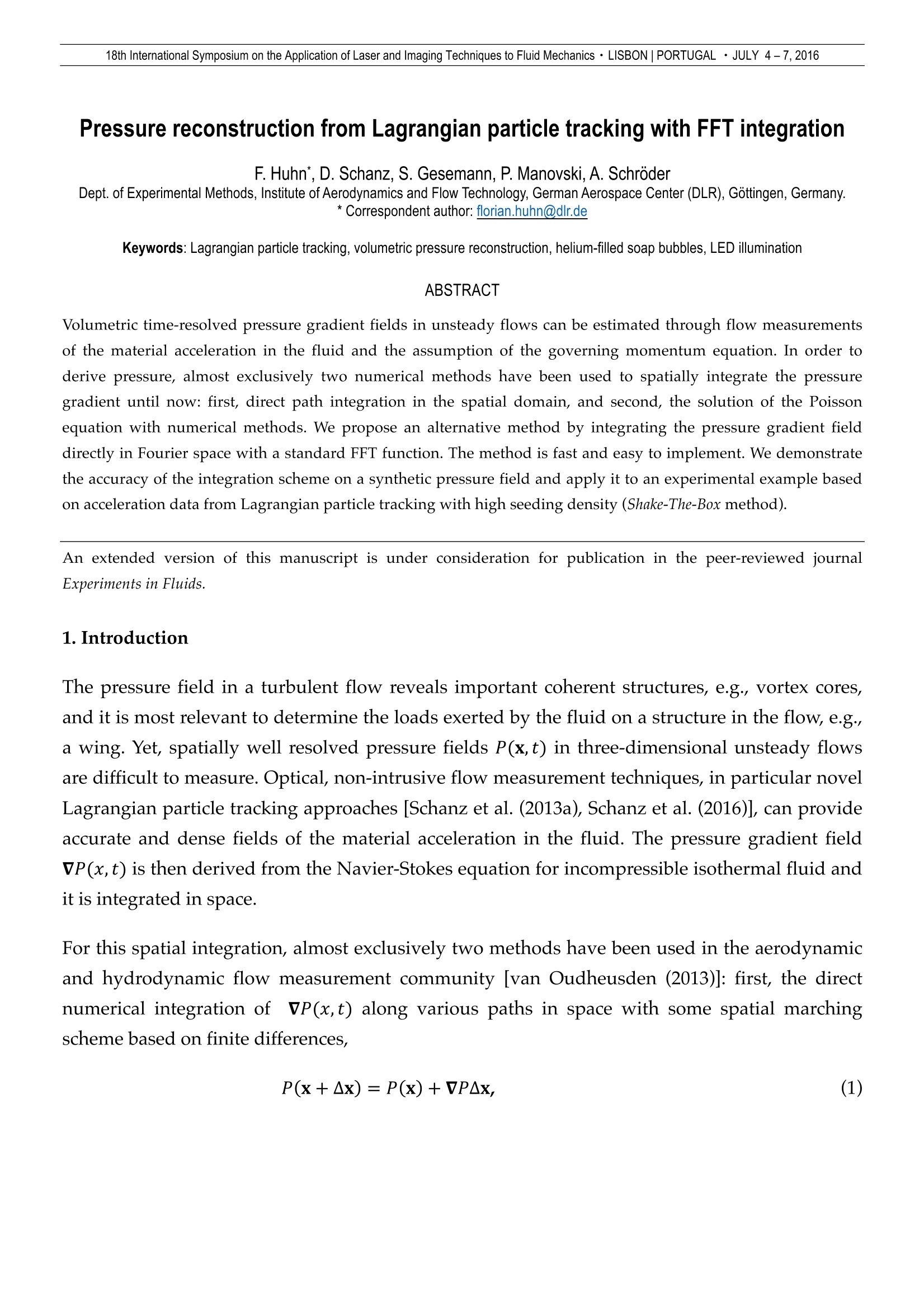
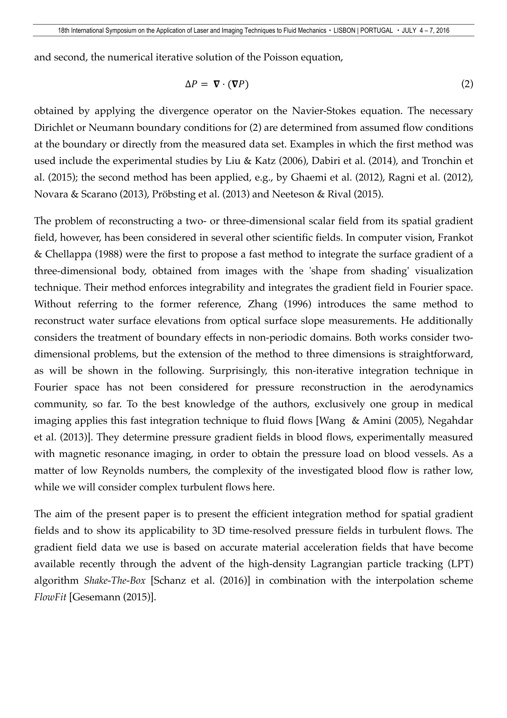
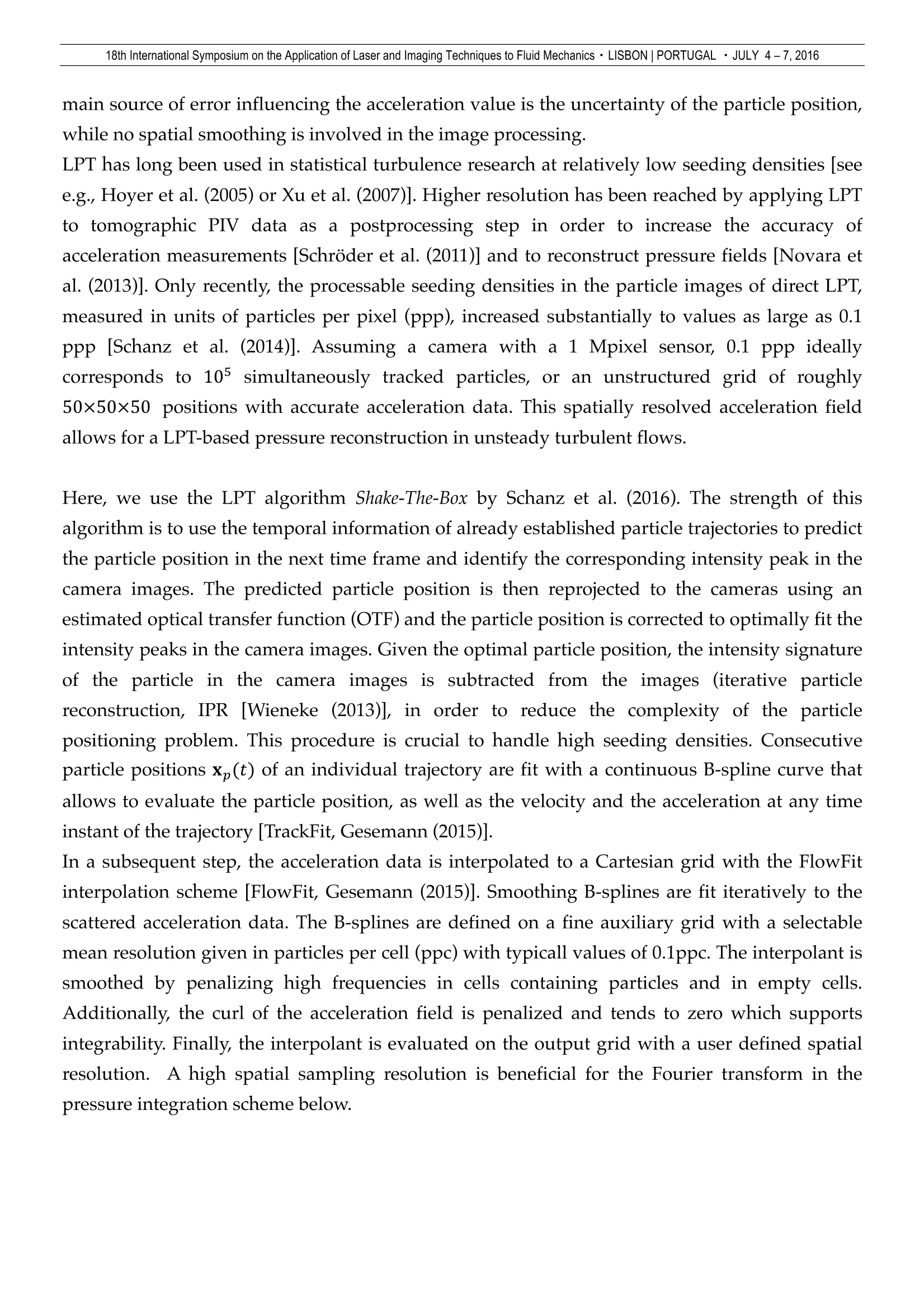
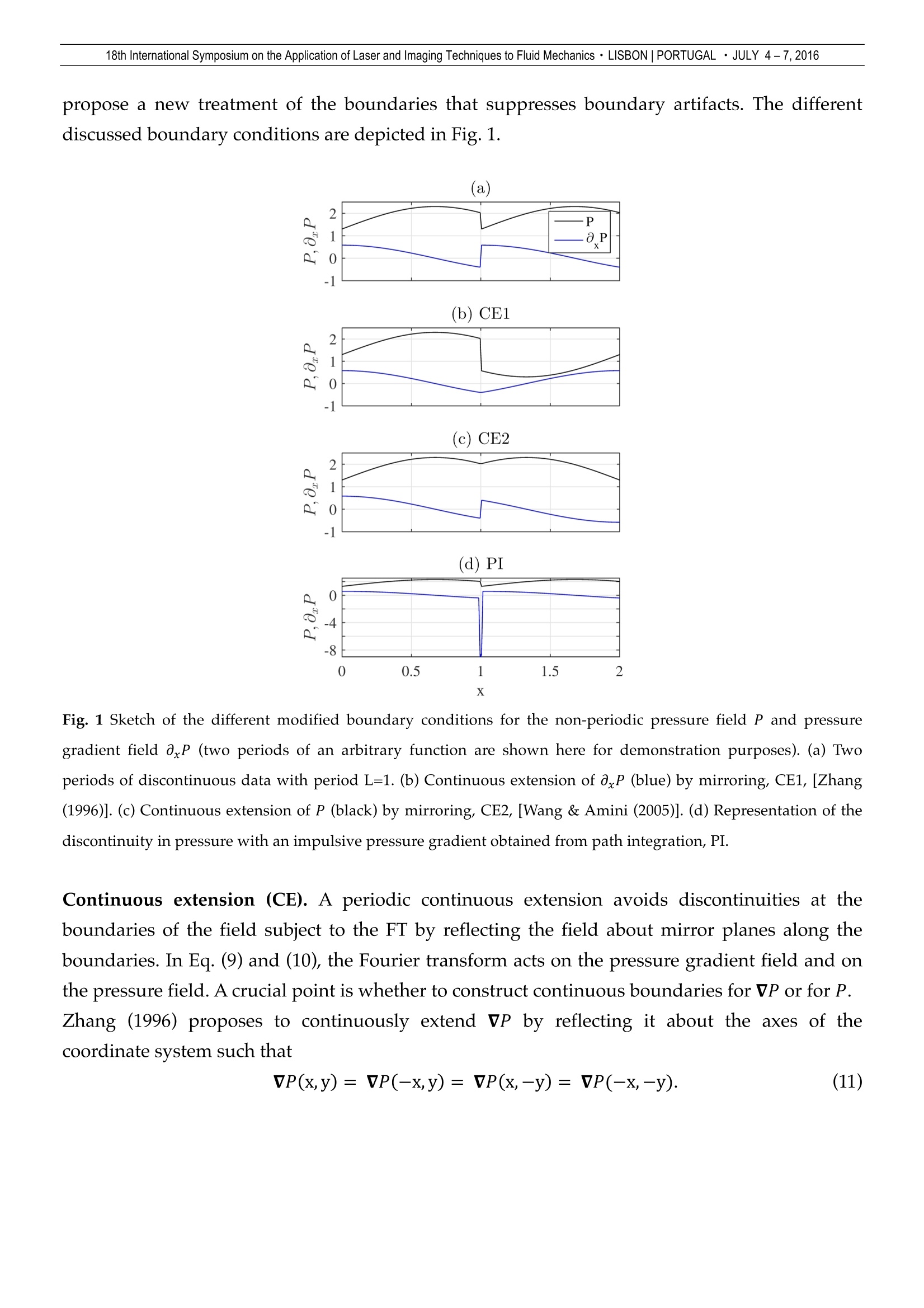
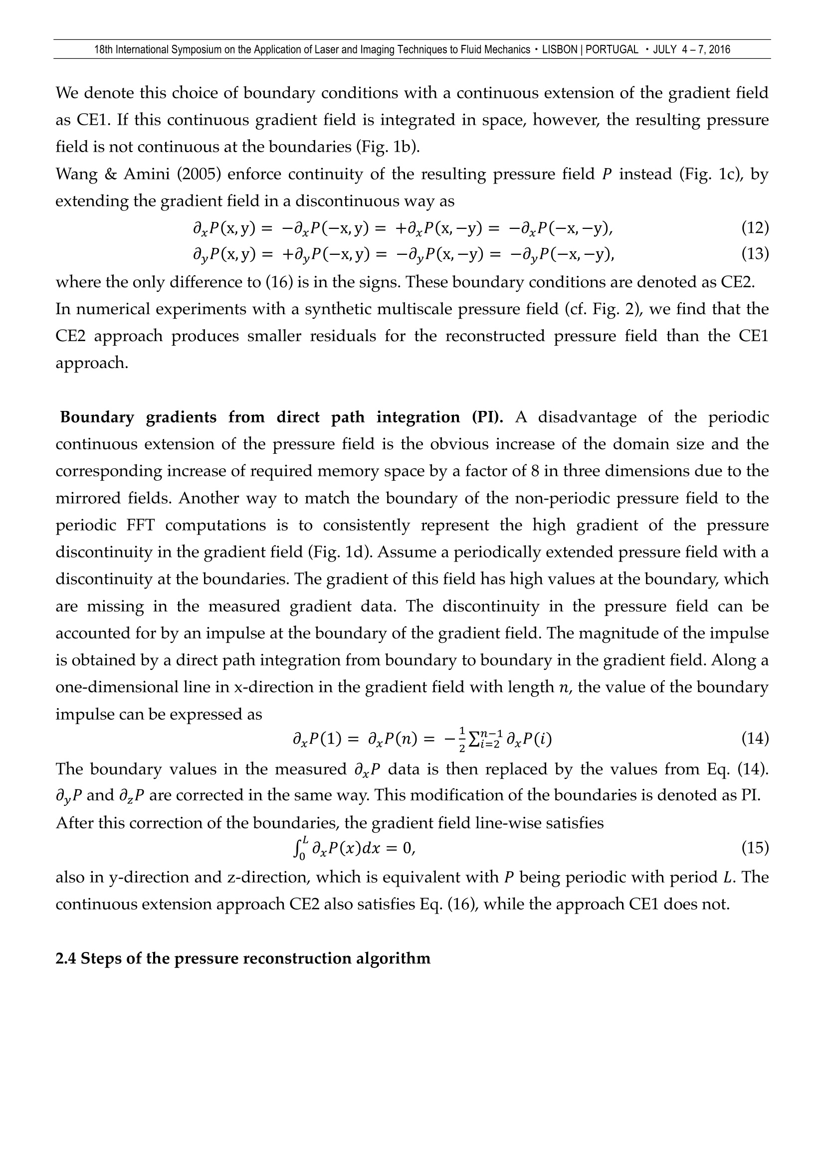
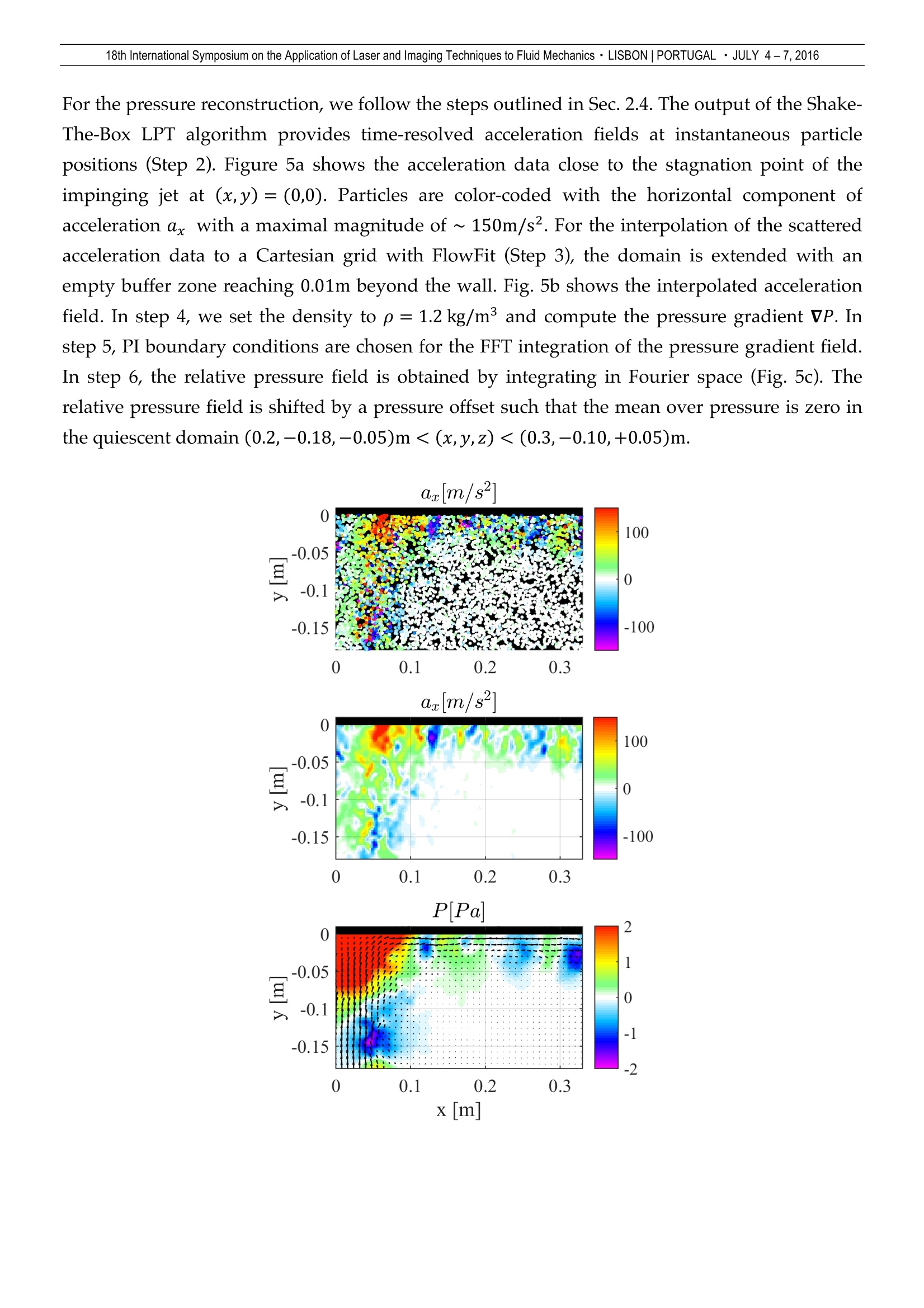
18th International Symposium on the Application of Laser and Imaging Techniques to Fluid Mechanics · LISBON |PORTUGAL · JULY 4-7, 2016 Pressure reconstruction from Lagrangian particle tracking with FFT integration F. Huhn*, D. Schanz, S. Gesemann, P. Manovski, A. Schroder Dept. of Experimental Methods, Institute of Aerodynamics and Flow Technology, German Aerospace Center (DLR), Gottingen, Germany.* Correspondent author: florian.huhn@dlr.de Keywords: Lagrangian particle tracking, volumetric pressure reconstruction, helium-filled soap bubbles, LED illumination ABSTRACT Volumetric time-resolved pressure gradient fields in unsteady flows can be estimated through flow measurementsof the material acceleration in the fluid and the assumption of the governing momentum equation. In order toderive pressure, almost exclusively two numerical methods have been used to spatially integrate the pressuregradient until now: first, direct path integration in the spatial domain, and second, the solution of the Poissonequation with numerical methods. We propose an alternative method by integrating the pressure gradient fielddirectly in Fourier space with a standard FFT function. The method is fast and easy to implement. We demonstratethe accuracy of the integration scheme on a synthetic pressure field and apply it to an experimental example basedon acceleration data from Lagrangian particle tracking with high seeding density (Shake-The-Box method). An extended version of this manuscript is under consideration for publication in the peer-reviewed journalExperiments in Fluids. 1. Introduction The pressure field in a turbulent flow reveals important coherent structures, e.g., vortex cores,and it is most relevant to determine the loads exerted by the fluid on a structure in the flow, e.g.,a wing. Yet, spatially well resolved pressure fields P(x,t) in three-dimensional unsteady flowsare difficult to measure. Optical, non-intrusive flow measurement techniques, in particular novelLagrangian particle tracking approaches [Schanz et al. (2013a), Schanz et al. (2016)], can provideaccurate and dense fields of the material acceleration in the fluid. The pressure gradient fieldVP(x,t) is then derived from the Navier-Stokes equation for incompressible isothermal fluid andit is integrated in space. For this spatial integration, almost exclusively two methods have been used in the aerodynamicand hydrodynamic flow measurement community [van Oudheusden (2013)]: first, the directnumerical integration of VP(x,t) along various paths in space with some spatial marchingscheme based on finite differences, and second, the numerical iterative solution of the Poisson equation, obtained by applying the divergence operator on the Navier-Stokes equation. The necessaryDirichlet or Neumann boundary conditions for (2) are determined from assumed flow conditionsat the boundary or directly from the measured data set. Examples in which the first method wasused include the experimental studies by Liu & Katz (2006), Dabiri et al. (2014), and Tronchin etal. (2015); the second method has been applied, e.g., by Ghaemi et al. (2012), Ragni et al. (2012),Novara & Scarano (2013), Probsting et al. (2013) and Neeteson & Rival (2015). The problem of reconstructing a two- or three-dimensional scalar field from its spatial gradientfield, however, has been considered in several other scientific fields. In computer vision, Frankot& Chellappa (1988) were the first to propose a fast method to integrate the surface gradient of athree-dimensional body, obtained from images with the 'shape from shading'visualizationtechnique. Their method enforces integrability and integrates the gradient field in Fourier space.Without referring to the former reference, Zhang (1996) introduces the same method toreconstruct water surface elevations from optical surface slope measurements. He additionallyconsiders the treatment of boundary effects in non-periodic domains. Both works consider two-dimensional problems, but the extension of the method to three dimensions is straightforward,as will be shown in the following. Surprisingly, this non-iterative integration technique inFourier space has not been considered for pressure reconstruction in the aerodynamicscommunity, so far. To the best knowledge of the authors, exclusively one group in medicalimaging applies this fast integration technique to fluid flows [Wang & Amini (2005), Negahdaret al. (2013)]. They determine pressure gradient fields in blood flows, experimentally measuredwith magnetic resonance imaging, in order to obtain the pressure load on blood vessels. As amatter of low Reynolds numbers, the complexity of the investigated blood flow is rather low,while we will consider complexturbulent flows here. The aim of the present paper is to present the efficient integration method for spatial gradientfields and to show its applicability to 3D time-resolved pressure fields in turbulent flows. Thegradient field data we use is based on accurate material acceleration fields that have becomeavailable recently through the advent of the high-density Lagrangian particle tracking (LPT)algorithm Shake-The-Box [Schanz et al. (2016)] in combination with the interpolation schemeFlowFit [Gesemann (2015)]. The paper is organized as follows. In Sec. 2, we recall the principles of pressure reconstructionfrom flow measurements and present the integration method of the pressure gradient.In Sec. 3,we show examples of pressure reconstruction for a synthetic pressure field to validate theintegration method, and in Sec. 4, we reconstruct the pressure field in an experimental turbulentflow. Finally, Sec. 5 summarizes the results. 2. Data and Methods 2.1 Momentum equation The momentum pu of a fluid parcel in an isothermal viscid Newtonian fluid evolves accordingto the Navier-Stokes equation with constant density p, constant viscosity u, and the material acceleration Du/Dt, i.e., theacceleration of a fluid parcel along its trajectory. Far from boundaries, the pressure gradient forcetypically dominates, such that for flows with high Reynolds number, the viscous term is small and a good estimate ofthe pressure gradient field can be obtained by where we denote the material (or Lagrangian) acceleration with a from here on. 2.1 Measurement of Lagrangian acceleration According to the term in brackets in Eq. (3), acceleration could simply be obtained from time-resolved velocity fields as measured with particle image velocimetry (PIV). PIV is a robustmethod to obtain time-resolved velocity fields from pairs of particle images. However, thisindirect acceleration measurement involves spatial and temporal derivatives of the velocity field(3). The derivatives enhance measurement noise in the velocity field, which can lead to noisyacceleration fields, and consequently to noisy pressure gradient fields. Additionally, the spatialsmoothing effect of the correlation window in the PIV technique may lead to an underestimationof the velocity gradient, and thus of the acceleration. Lagrangian particle tracking (LPT) overcomes these problems by tracking individual tracerparticles, such that entire time-resolved trajectories of particles x,(Xo,to,t) can be measured.Velocity and acceleration are determined as point measurements at the well-defined position ofan individual tracer. Acceleration at particle positions is obtained as a(x,,t)=dx,(t)/dt2. The main source of error influencing the acceleration value is the uncertainty of the particle position,while no spatial smoothing is involved in the image processing. LPT has long been used in statistical turbulence research at relatively low seeding densities [seee.g., Hoyer et al. (2005) or Xu et al. (2007)]. Higher resolution has been reached by applying LPTto tomographic PIV data as a postprocessing step in order to increase the accuracy ofacceleration measurements [Schroder et al. (2011)] and to reconstruct pressure fields [Novara etal. (2013)]. Only recently, the processable seeding densities in the particle images of direct LPT,measured in units of particles per pixel (ppp), increased substantially to values as large as 0.1ppp [Schanz et al.(2014)]. Assuming a camera with a 1 Mpixel sensor, 0.1 ppp ideallycorresponds to 105 simultaneously tracked particles, or an unstructured grid of roughly50×50×50 positions with accurate acceleration data. This spatially resolved acceleration fieldallows for a LPT-based pressure reconstruction in unsteady turbulent flows. Here, we use the LPT algorithm Shake-The-Box by Schanz et al. (2016). The strength of thisalgorithm is to use the temporal information of already established particle trajectories to predictthe particle position in the next time frame and identify the corresponding intensity peak in thecamera images. The predicted particle position is then reprojected to the cameras using anestimated optical transfer function (OTF) and the particle position is corrected to optimally fit theintensity peaks in the camera images. Given the optimal particle position, the intensity signatureof the particle in the camera images is subtracted from the images (iterative particlereconstruction, IPR [Wieneke (2013)], in order to reduce the complexity of the particlepositioning problem. This procedure is crucial to handle high seeding densities. Consecutiveparticle positions x(t) of an individual trajectory are fit with a continuous B-spline curve thatallows to evaluate the particle position, as well as the velocity and the acceleration at any timeinstant of the trajectory [TrackFit, Gesemann (2015)]. In a subsequent step, the acceleration data is interpolated to a Cartesian grid with the FlowFitinterpolation scheme [FlowFit, Gesemann (2015)]. Smoothing B-splines are fit iteratively to thescattered acceleration data. The B-splines are defined on a fine auxiliary grid with a selectablemean resolution given in particles per cell (ppc) with typicall values of 0.1ppc. The interpolant issmoothed by penalizing high frequencies in cells containing particles and in empty cells.Additionally, the curl of the acceleration field is penalized and tends to zero which supportsintegrability. Finally, the interpolant is evaluated on the output grid with a user defined spatialresolution. A high spatial sampling resolution is beneficial for the Fourier transform in thepressure integration scheme below. 2.2 Integration scheme for pressure reconstruction Following Frankot & Chellappa (1988), we obtain the pressure field P(x) by integrating themeasured three-dimensional pressure gradient fields in Fourier space and by transforming back to normal space For a short derivation of (9), see Ref. [Rocholz (2008)]. The tilde denotes a Fourier transformedfunction, e.g., x=FT(P), FT-1 is the inverse Fourier transform, and ky,k,kz are thecomponents of the wave number vector k. In (9), the separation of the curl-free longitudinalcomponent of the vector field corresponds to a projection of the pressure gradient onto thek-vectork k·vP]/|k|2, and the integration in space corresponds to a division by ik. Equation (9) has a singularity at k=0. In order to handle this, the amplitude for the constantcomponent is set to zero, P(k=0)=0. By this operation, the amplitudes of the constantcomponent of the three pressure gradients is lost. Below, we set boundary conditions at theperiodic domain that account for the global linear pressure gradient. Finally, in order to obtain total pressure, the integration constant, a constant pressure offset Po,obtained from additional measurements or from theoretical considerations at the boundaries, isadded to the relative pressure field P(x). 2.3 Boundary conditions for periodic domain The Fourier transform assumes an infinite periodic domain for the transformed fields, acondition that is typically not met by measurement data. A continuous extension of the field bymirroring the data has been proposed to minimize boundary artifacts due to non-periodicity ofthe data [Zhang (1996), Wang & Amini (2005)]. In the following, we discuss this approach and propose a new treatment of the boundaries that suppresses boundary artifacts. The differentdiscussed boundary conditions are depicted in Fig. 1. X Fig. 1 Sketch of the different modified boundary conditions for the non-periodic pressure field Pand pressuregradient field axP (two periods of an arbitrary function are shown here for demonstration purposes). (a) Twoperiods of discontinuous data with period L=1. (b) Continuous extension of oxP (blue) by mirroring, CE1, [Zhang(1996)]. (c) Continuous extension of P (black) by mirroring, CE2, [Wang & Amini (2005)]. (d) Representation of thediscontinuity in pressure with an impulsive pressure gradient obtained from path integration, PI. Continuous extension (CE). A periodic continuous extension avoids discontinuities at theboundaries of the field subject to the FT by reflecting the field about mirror planes along theboundaries. In Eq. (9) and (10), the Fourier transform acts on the pressure gradient field and onthe pressure field. A crucial point is whether to construct continuous boundaries for VP or for P.Zhang (1996) proposes to continuously extend VP by reflecting it about the axes of thecoordinate system such that We denote this choice of boundary conditions with a continuous extension of the gradient fieldas CE1. If this continuous gradient field is integrated in space, however, the resulting pressurefield is not continuous at the boundaries (Fig.1b). Wang & Amini (2005) enforce continuity of the resulting pressure field P instead (Fig. 1c), byextending the gradient field in a discontinuous way as where the only difference to (16) is in the signs. These boundary conditions are denoted as CE2.In numerical experiments with a synthetic multiscale pressure field (cf. Fig.2), we find that theCE2 approach produces smaller residuals for the reconstructed pressure field than the CE1approach. Boundary gradients from direct path integration (PI). A disadvantage of the periodiccontinuous extension of the pressure field is the obvious increase of the domain size and thecorresponding increase of required memory space by a factor of 8 in three dimensions due to themirrored fields. Another way to match the boundary of the non-periodic pressure field to theperiodic FFT computations is to consistently represent the high gradient of the pressurediscontinuity in the gradient field (Fig.1d). Assume a periodically extended pressure field with adiscontinuity at the boundaries. The gradient of this field has high values at the boundary, whichare missing in the measured gradient data. The discontinuity in the pressure field can beaccounted for by an impulse at the boundary of the gradient field. The magnitude of the impulseis obtained by a direct path integration from boundary to boundary in the gradient field.Along aone-dimensional line in x-direction in the gradient field with length n, the value of the boundaryimpulse can be expressed as The boundary values in the measured axP data is then replaced by the values from Eq. (14).0,P ando P are corrected in the same way. This modification of the boundaries is denoted as PI.After this correction of the boundaries, the gradient field line-wise satisfies also in y-direction and z-direction, which is equivalent with P being periodic with period L. Thecontinuous extension approach CE2 also satisfies Eq. (16), while the approach CE1 does not. 2.4 Steps of the pressure reconstruction algorithm Including the LPT measurement, we summarize the pressure reconstruction with the followingsteps: 1. Reconstruct particle trajectories from time-resolved particle images of at least threecameras using the STB algorithm [Schanz et al. (2016)]. 2!.. Fit an interpolating continuous function consisting of 1D cubic B-splines to the trajectoriesand differentiate twice w.r.t. time to obtain the material acceleration at particle positions(TrackFit, Gesemann (2015)). 3.Interpolate the acceleration, given on an unstructured grid, to a fine Cartesian grid, using3D cubic B-splines and penalyzing the curl of the acceleration field (FlowFit, Gesemann(2015)). 4.Neglect the viscous term in (3), assume constant density p and compute VP (6-8). 5.Modify VP by applying the CE or PI method for periodic spatial boundary conditionsfrom Sec.2.3, in order to avoid boundary artifacts. 6i.. Compute the Fourier transforms of VP, evaluate (9), set P(k=0)= 0, and transform back,using a Fast-Fourier-Transform (FFT) function. 7. Add a constant pressure offset Po to obtain total pressure. Regardless of the exact way to obtain the pressure gradient on a Cartesian grid, be it a differentmeasurement technique or the additional consideration of theoretical models,, e.g. acompressible flow with varying density, the integration method is anyhow applicable, startingfrom step 5. 3. Synthetic pressure field In order to validate the accuracy of the integration method, we create a three-dimensionalsynthetic pressure field on a cubic 257×257×257 domain as ground truth data, compute thespatial gradient and reconstruct the pressure field. A direct comparison of the original and thereconstructed pressure field reveals the accuracy of the integration. In order to generate thesynthetic pressure field, uniformly distributed noise in Fourier space is multiplied with anormalized correlation kernel of the form f(k)= exp(-a|k|2). The slow decay of the kernelwith an exponent 1/2 generates a wide range of scales, since turbulent pressure fields typicallyinclude large scale gradients as well as small scale structures related to vortices. When theparameter a is increased, high wavenumbers are damped and the synthetic pressure field showslarger spatial structures. For the test case shown, the parameter is set to α =6.7, resulting in aspatial structure of the pressure field as shown in Fig. 2a (central x-y plane). The gradient of the periodic pressure field is computed in Fourier space by multiplying with ik,then, a non-periodic 100×100×100 subdomain is cropped in real space for the test. Pressure isreconstructed from the gradient fields, with and without accounting for periodic boundaryconditions. With unchanged boundaries, i.e. non-periodic boundaries, the reconstructed pressurefield significantly deviates from the original field (not shown). When the gradient field iscontinuously extended according to CE1 boundary conditions (11), the deviation is still large.Figure 2b shows the difference between original and reconstructed pressure field. In contrast,when the boundaries are modified according to the CE2 method (12-13) or the PI method (14),the reconstructed pressure field agrees with the original field within an error of less than 1%.Figures 2c and 2d show the small difference between original and reconstructed pressure field,profiles along a section in x-direction (dashed line) show the small relative error (Fig. 2e and 2f). Fig. 2 (a) Synthetic three-dimensional pressure field (central plane) constructed as correlated noise. (b-d) Differencefields between reconstructed pressure field P. and ground truth data P for different boundary conditions. Samecolorbar for (a,b) and (c,d). (e,f) Relative error along a section (dashed line) for CE2 and PI boundary conditions. Noise, always present in measurement data, is added to the synthetic pressure gradient fields toassess the effect of noise on the accuracy of the pressure field. Noise fields are created in thesame way as the pressure field, i.e., as correlated noise with a correlation kernel in Fourier spacef(k)= exp(-a|k|2). Fig. 3 exemplarily shows the clean pressure gradient field oP together with the most extreme tested added noise field. Fig. 3 (a) Clean synthetic pressure gradient field oxP and (b) added noise field with largest tested spatial scaleparameter a =3.3 and largest tested relative noise amplitude Onoise/op=0.4. The amplitude and the spatial scale of the added noise are varied and the residual betweenreconstructed and original pressure field are analyzed. For PI boundary conditions, theboundary voxels in the reconstructed pressure field is typically strongly biased (Fig. 2c) due tothe imposed boundary condition, and is therefore neglected in the computation of the error.Figure 4 shows the expected behavior that the error in the reconstructed pressure fields increasesmonotonically with increasing noise added to the pressure gradient field. In the most extremecase (large amplitude and large spatial scale of the noise, cf. Fig. 3), the added noise leads to100% error of the reconstructed pressure field, i.e., drastically distorts the reconstructed pressurefield. For moderate noise, the residual linearly decreases, converging to the error of <1% for thenoise free case. The spatial scale of the added noise has a clear influence on the resulting error ofthe reconstructed pressure field. At the same relative noise amplitude, the error increases withincreasing spatial scale of the noise. This is expected, since the integration (division by ik) dampssmall spatial scales more than large spatial scales. Overall, the two most promising boundaryconditions (PI and CE2) perform equally well, with a tendency of the CE2 boundary conditions to cause slightly smaller errors in the reconstructed pressure field, at the cost of a eight timeshigher data volume (mirrored field) that has to be processed. noisevp Fig. 4 Relative residual between original and reconstructed pressure field derr/op=rms(Pr-P)/rms(P) dependingon added noise with relative amplitude Onoise/op and spatial scale parameter a= 1.1 (solid line), a =1.7 (dashedline) and a =3.3(dash-dotted line). 4. Experimental pressure field- Impinging jet The presented integration method for the pressure gradient field is applied to an experimentaldata set. In the experiment, an air jet generated by a fan (PHYWE-02742-93, upper and lowerscreen removed) with a nozzle exit diameter of D= 11cm and an exit velocity of U~ 5m/s hitsa flat acrylic glass plate at a distance of H = 55cm, H/D =5, and at an angle of 0 = 90°. In thelarge measurement volume adjacent to the wall (450×500×150mm) the flow is seeded with~180,000 helium-filled soap bubbles (HFSB) with a diameter of ~ 400um (LaVision HFSBgenerator) and a mean particle distance of d=6.8mm. Six high-speed cameras (PCO dimax,2016×2016 pix2) record particle images at a frame rate of f= 1kHz at full frame size withexposure time of 130us. The six cameras are positioned in an in-line configuration and orientedin a way that lines of sight are tangential to the flat plate. The HFSBs are illuminated by a pulsedLED array driven at 1kHz with a voltage of 44V, a current of 90A, and a pulse width of At =100us (10% duty cycle). For the pressure reconstruction, we follow the steps outlined in Sec. 2.4. The output of the Shake-The-Box LPT algorithm provides time-resolved acceleration fields at instantaneous particlepositions (Step 2). Figure 5a shows the acceleration data close to the stagnation point of theimpinging jet at (x,y)=(0,0). Particles are color-coded with the horizontal component ofacceleration ax with a maximal magnitude of ~150m/s2. For the interpolation of the scatteredacceleration data to a Cartesian grid with FlowFit (Step 3), the domain is extended with anempty buffer zone reaching 0.01m beyond the wall. Fig.5b shows the interpolated accelerationfield. In step 4, we set the density to p = 1.2 kg/m’ and compute the pressure gradient VP. Instep 5, PI boundary conditions are chosen for the FFT integration of the pressure gradient field.In step 6, the relative pressure field is obtained by integrating in Fourier space (Fig.5c). Therelative pressure field is shifted by a pressure offset such that the mean over pressure is zero inthe quiescent domain (0.2,-0.18,-0.05)m <(x,y,z)<(0.3,-0.10,+0.05)m. Fig. 5 (a) Particles color-coded with horizontal acceleration ax in a slice -10mm
确定


还剩13页未读,是否继续阅读?

产品配置单


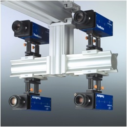
北京欧兰科技发展有限公司为您提供《流场中压力场检测方案(粒子图像测速)》,该方案主要用于其他中压力场检测,参考标准--,《流场中压力场检测方案(粒子图像测速)》用到的仪器有体视层析粒子成像测速系统(Tomo-PIV)、LaVision DaVis 智能成像软件平台
推荐专场


相关方案
更多
该厂商其他方案
更多