


方案详情
文
Geostrophic adjustment of an isolated axisymmetric lens was examined to better understand the
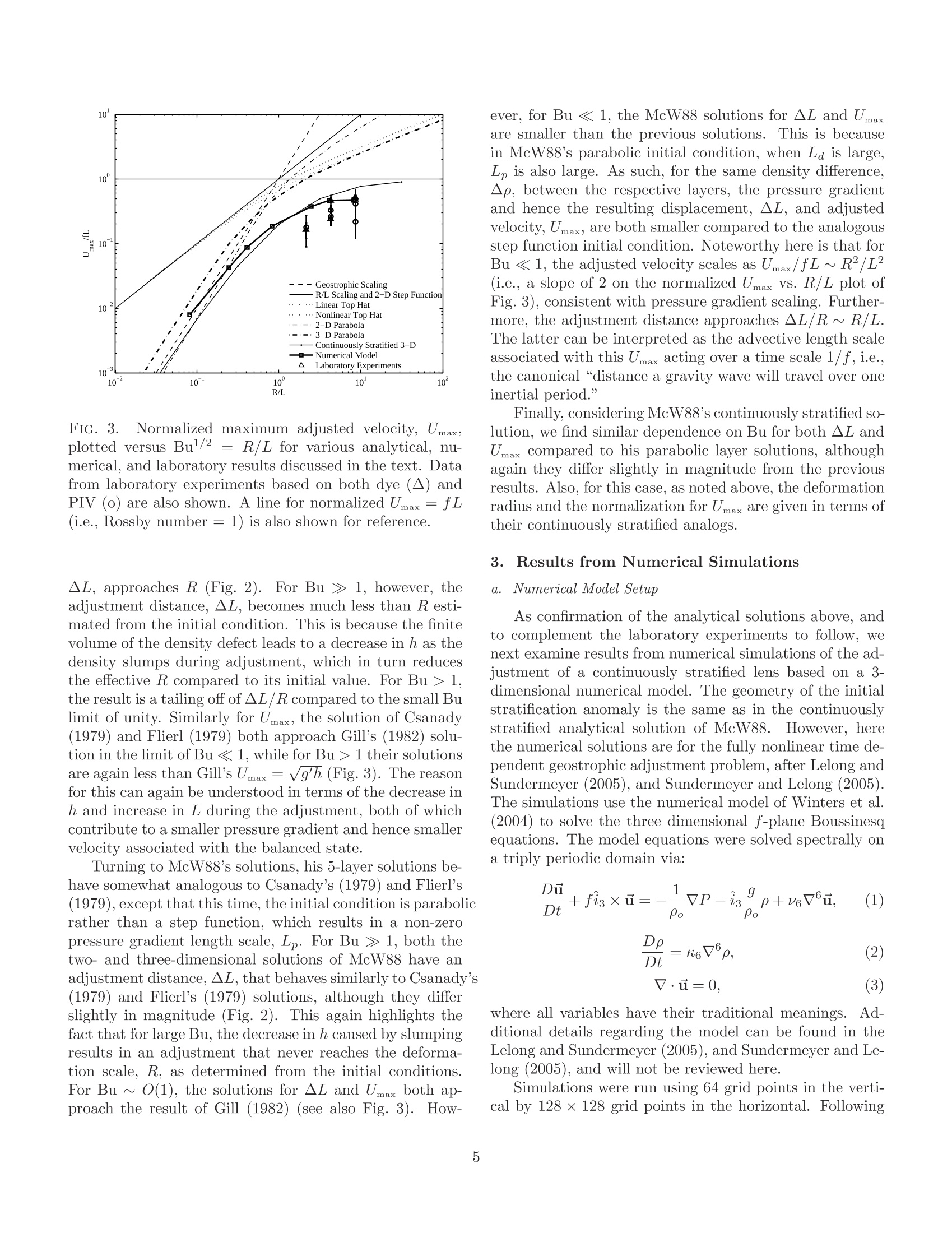
dependence of radial displacements and the adjusted velocity on Burger number and the geometry
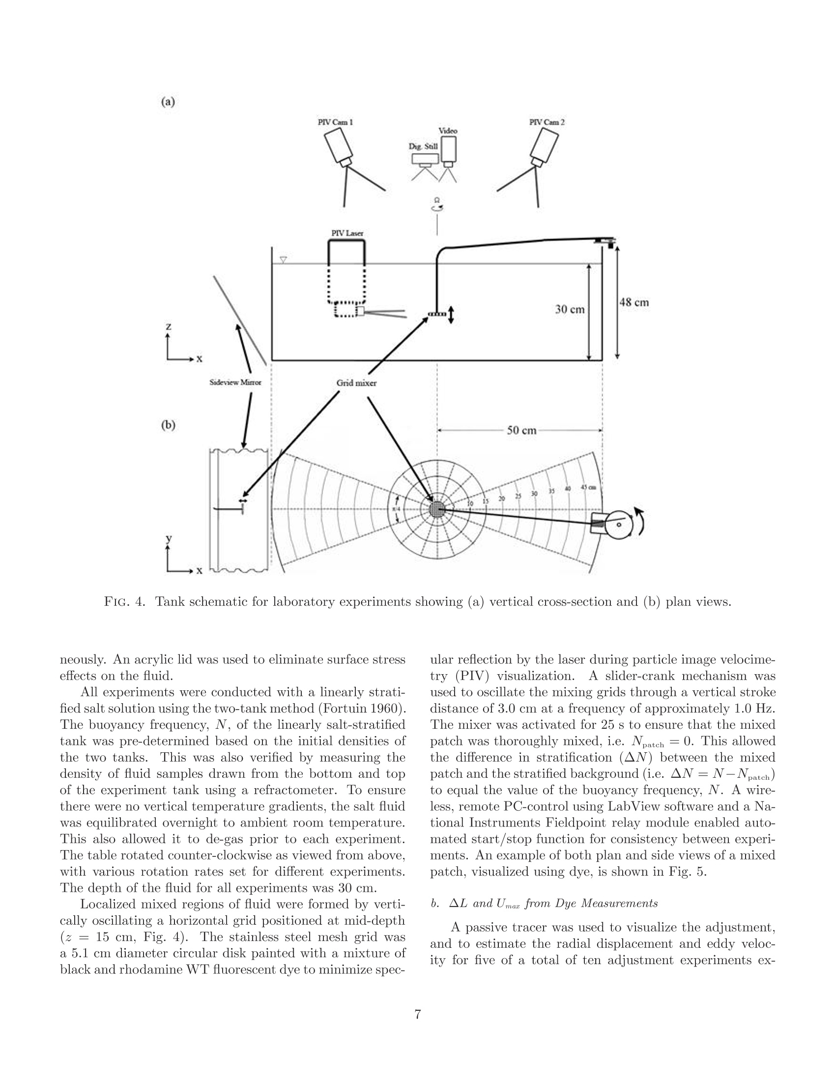
of initial conditions. The behavior of the adjustment was examined using laboratory experiments
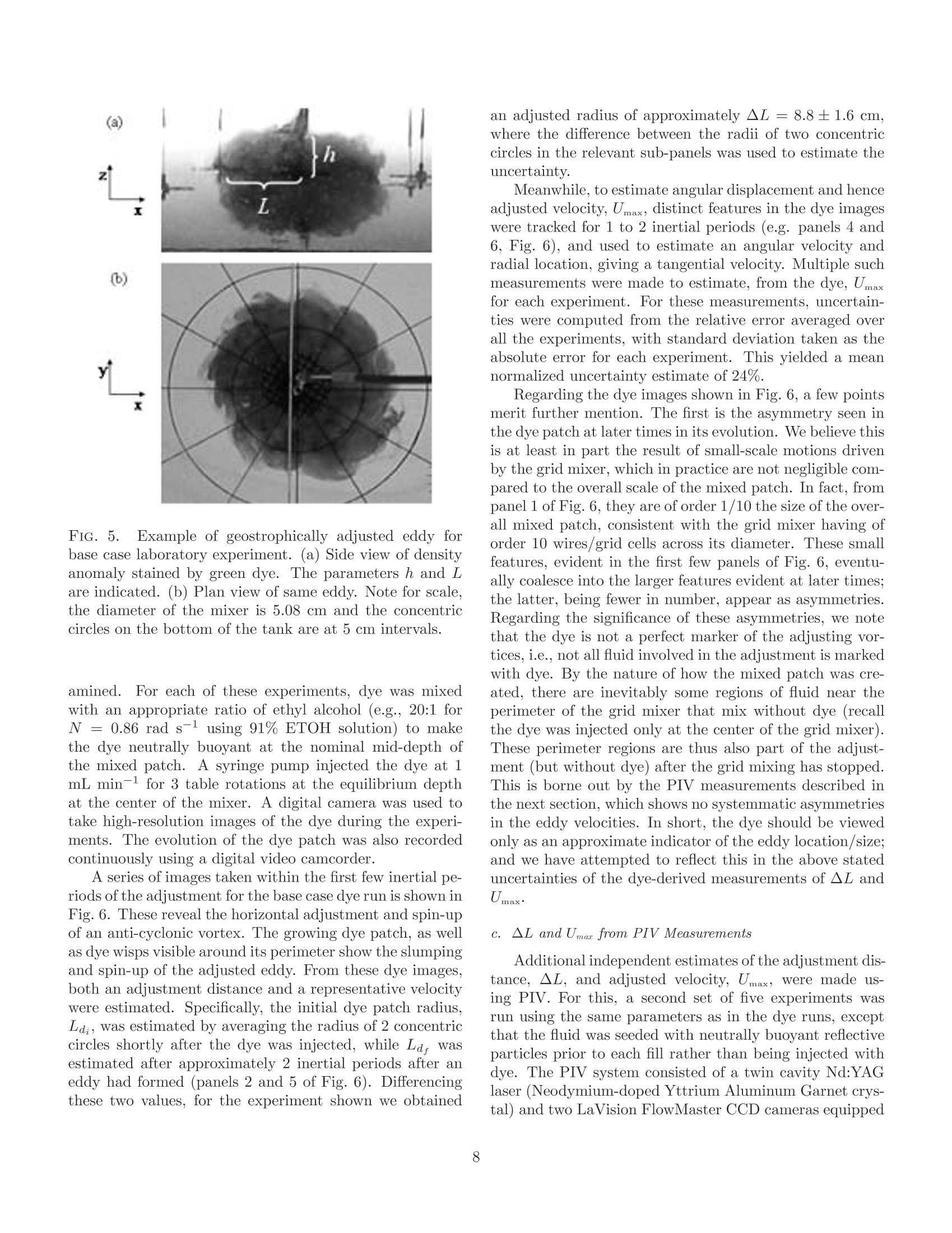
and numerical simulations, which were in turn compared to published analytical solutions. Three
defining length scales of the initial conditions were used to distinguish between various asymptotic
behaviors for large and small Burger number: the Rossby radius of deformation, the horizontal
length scale of the initial density defect, and the horizontal length scale of the initial pressure
gradient. Numerical simulations for the fully nonlinear time dependent adjustment agreed both
qualitatively and quantitatively with analogous analytical solutions. For large Burger number,
similar agreement was found in laboratory experiments. Results show that a broad range of final
states can result from different initial geometries, depending on the values of the relevant length
scales, and the Burger number computed from initial conditions. For Burger number much larger
or smaller than unity, differences between different initial geometries can readily exceed an order of
magnitude for both displacement and velocity.
方案详情

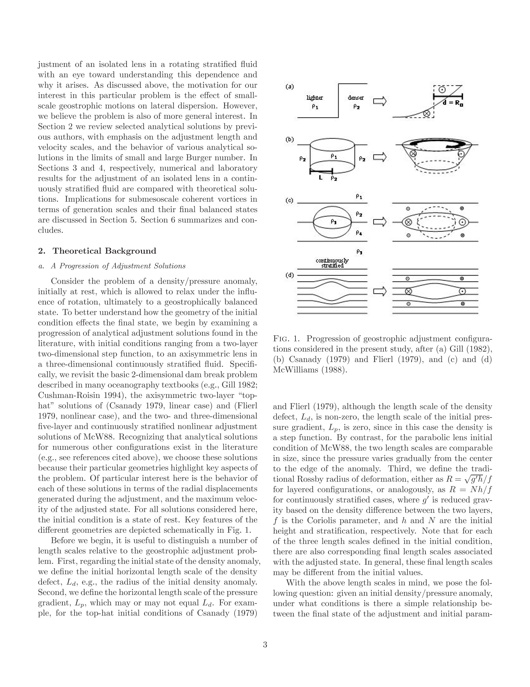
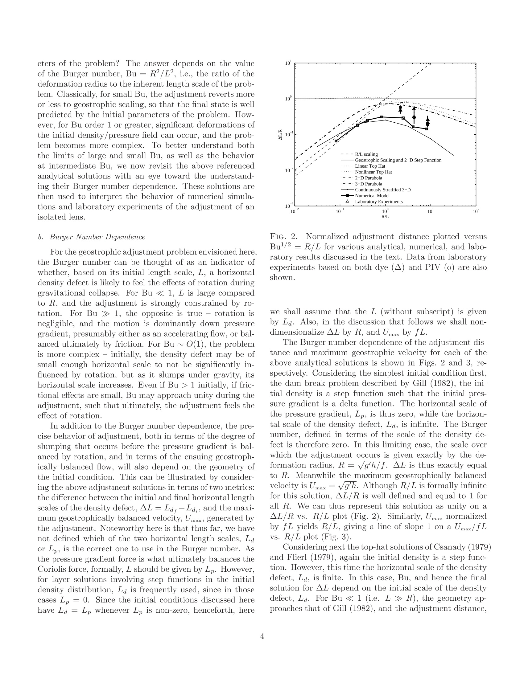
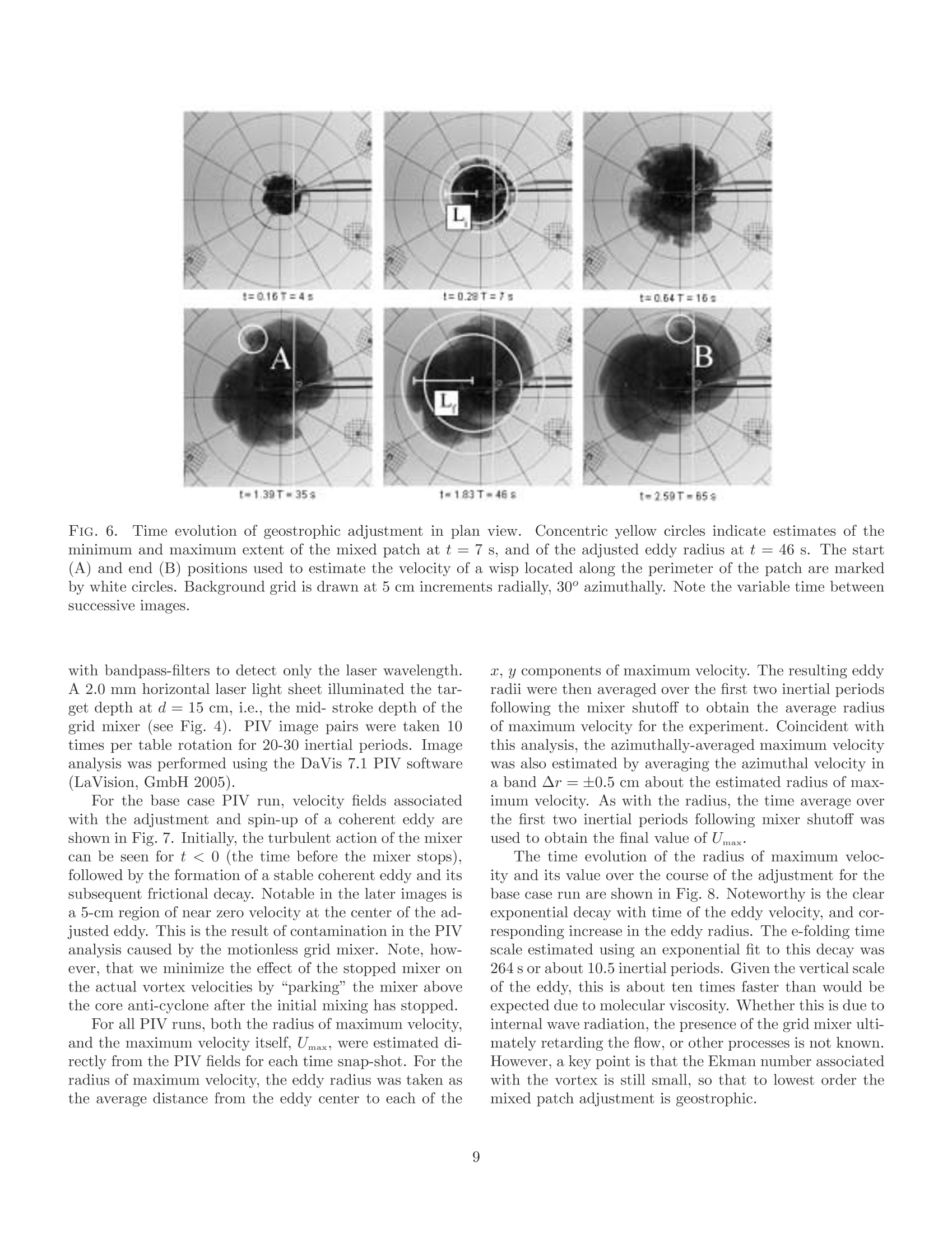
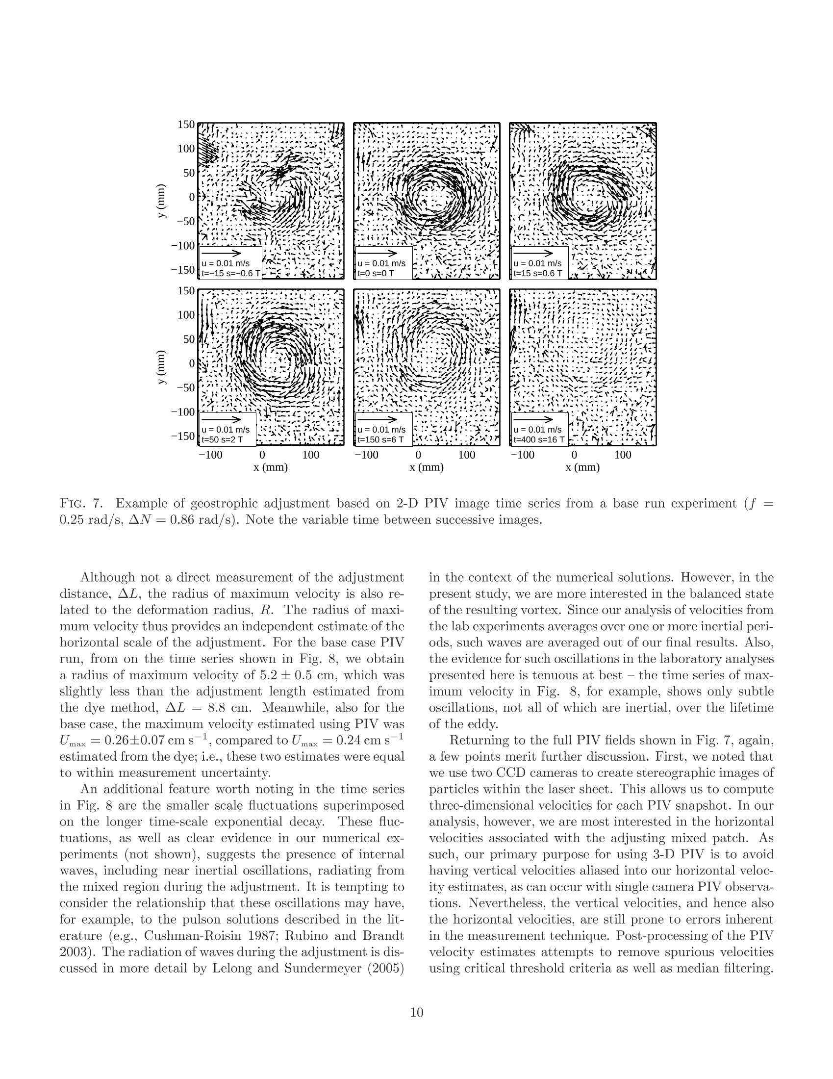
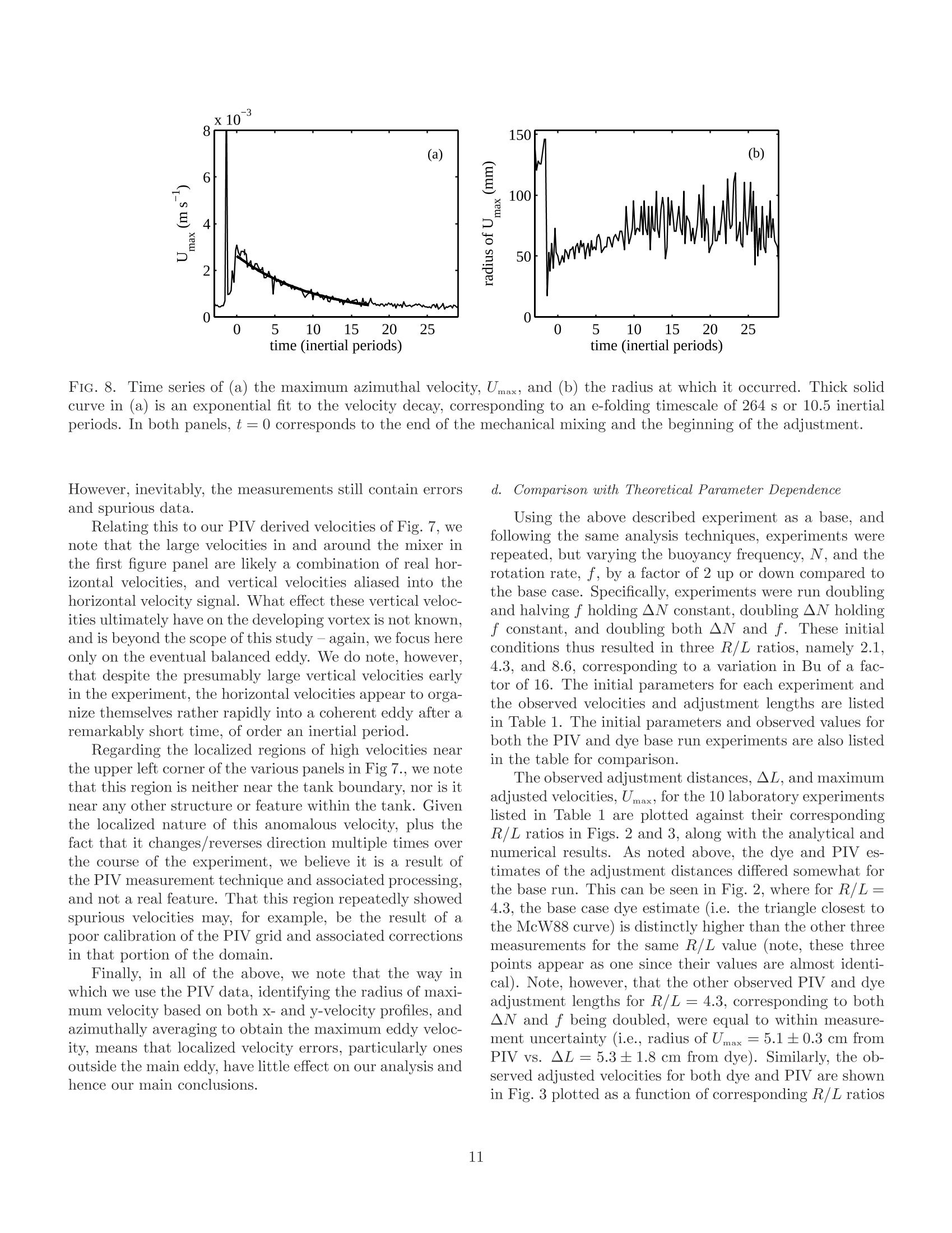
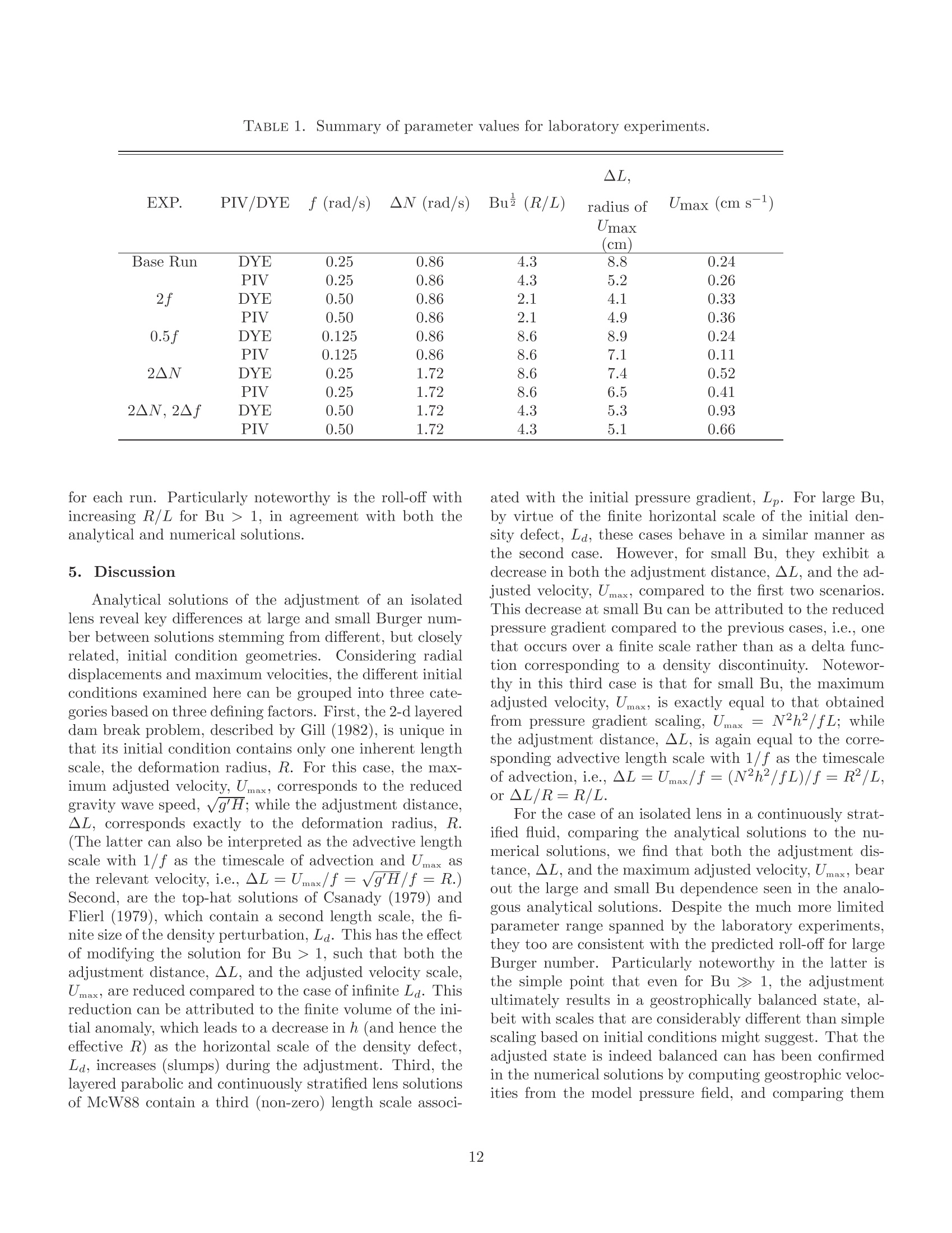
Submitted to: J. Phys.Oceanogr. TABLE 1. Summary of parameter values for laboratory experiments. On the Geostrophic Adjustment of an Isolated Lens:Dependence on Burger Number and Initial Geometry GRANT A. STUART MILES A. SUNDERMEYER * University of Massachusetts Dartmouth,Dartmouth, MA, USA and DAVE HEBERT Graduate School of Oceanography, University of Rhode Island, Narragansett, RI, USA ABSTRACT Geostrophic adjustment of an isolated axisymmetric lens was examined to better understand thedependence of radial displacements and the adjusted velocity on Burger number and the geometryof initial conditions. The behavior of the adjustment was examined using laboratory experimentsand numerical simulations, which were in turn compared to published analytical solutions.TThreedefining length scales of the initial conditions were used to distinguish between various asymptoticbehaviors for large and small Burger number: the Rossby radius of deformation, the horizontallength scale of the initial density defect, and the horizontal length scale of the initial pressuregradient. Numerical simulations for the fully nonlinear time dependent adjustment agreed bothqualitatively and quantitatively with analogous analytical solutions.For large Burger number,similar agreement was found in laboratory experiments. Results show that a broad range of finalstates can result from different initial geometries, depending on the values of the relevant lengthscales, and the Burger number computed from initial conditions. For Burger number much largeror smaller than unity, differences between different initial geometries can readily exceed an order ofmagnitude for both displacement and velocity. 1L.. Introduction C.t.Motivation and Background In classic geostrophic adjustment, an initially unbal-anced state in the form of a front or lens is allowed tocollapse under the combined influence of gravity and ro-tation.Through a combination of slumping and radia-tion of internal waves, a balanced or quasi-balanced flow isformed in which the pressure gradient is balanced by rota-tion and possibly nonlinear terms. In the textbook prob-lem, the final state can be predicted from initial parametersin terms of the Rossby radius of deformation, given by thedistance a gravity wave will travel in one inertial period,and geostrophic velocity scaling, which represents a bal-ance between the Coriolis and pressure gradient terms inthe momentum equation. When the scale of the adjusting density field is largecompared to the deformation radius, the solution is gener-ally considered to be well described in terms of such scaling.However, when the horizontal scale of the initial densityanomaly is of the same order or less than the deformationradius, the adjustment is somewhat more complicated. Insuch cases, the adjustment process itself can generate order one changes in the horizontal and vertical scales of the ini-tial pressure anomaly, such that the parameters associatedwith the final state are significantly different than those as-sociated with the initial state. The resultant flow may stillbe geostrophically balanced. However, the magnitude ofthe balanced flow will depend on a variety factors, includ-ing the scales and specific geometry of the initial densitydefect. The general problem of geostrophic adjustment datesback to Rossby (1937,1938) and has been well studied inthe literature since then. Reviews of the classic adjustmentproblem, as well as many of its variants, may be found,for example, in Blumen (1972), Gill (1982), McWilliams(1985), and Flierl (1987). Subsequent studies have con-tinued to relate the basic principles to a range of oceano-graphic phenomena, including the adjustment of densityfronts and their associated meanders (e.g., Ou 1984; van-Heijst 1985; Garvine 1987; Spall 1995; Blumen and Wu1995), the ocean response to storms (e.g., Geisler 1970;Price 1981), the dynamics of dense water outflows (e.g.,Price and O'Neil Baringer 1994; Cenedese et al. 2004),and ocean convection (e.g., Killworth 1979; Hermann andOwens 1993; Whitehead et al. 1996; Rubino et al. 2007), to name a few. In the present study, we are interested in one sub-classof the problem,the adjustment of an isolated lens in a con-tinuously stratified fluid. This configuration can arise, forexample, as the result of localized internal wave breaking inthe ocean interior. Evidence of patchy mixing in the oceanhas been reported by numerous investigators (e.g., Grantet al. 1968; Woods and Wiley 1972; Gregg 1980; Gregget al. 1986; Alford and Pinkel 2000; Oakey and Greenan2004; Sundermeyer et al. 2005). Such localized mixingcan lead to gravitational adjustment of the mixed regions,which, under the influence of rotation, can in turn leadto small-scale geostrophically balanced flows (e.g., Garrettand Munk 1972; McWilliams 1985). These small-scale bal-anced motions have been referred to in the literature asthe vortical mode, semi-permanent fine structure, pancakeeddies, or blini (e.g., Kunze 2001; Polzin et al. 2003). Inpractice, they have aspect ratios of order f/N, similar tothe internal wave field, with scales ranging from hundredsof meters to many kilometers horizontally, and of order me-ters to tens of meters vertically. As described by Sunder-meyer et al. (2005), and Sundermeyer and Lelong (2005),the motions from many of these adjustments can also con-tribute significantly to submesoscale lateral dispersion inthe ocean interior. It is the latter that motivates our par-ticular interest in the displacements generated by such ed-dies. In addition to localized internal wave breaking, nu-merous other processes have been hypothesized to con-tribute to vortical mode energy in the ocean. These in-clude the downscale transfer of variance associated withthe potential enstrophy cascade of geostrophic turbulence(e.g., Charney 1971), detrainment and subduction of sur-face mixed layer water (e.g., Stommel 1979; Marshallet al.1993; Spall 1995), and intensified mixing near topogra-phy (e.g., D'Asaro 1988; Kunze and Sanford 1993).. Inthe present context, however, we restrict our attention tothe geometry most appropriate to the adjustment of mixedpatches generated by diapycnal mixing events.For thisgeneration mechanism, the so-called “s-vortex”describedby Morel and McWilliams (1997) is particularly appropri-ate. Such a vortex is formed when a localized region ofreduced stratification is allowed to adjust under the in-fluence of rotation to form a core anti-cyclone (associatedwith vortex compression at the center of the mixed region),sandwiched above and below by two weaker cyclones (as-sociated with vortex stretching above and below the mainmixed region). Other vortex geometries (e.g., without the accompany-ing cyclones above and below, of varying steepness, and/orisolated vs. non-isolated) have also been used to modeloceanic eddies in a variety of contexts and scales, fromMediterranean eddies (e.g., Armi and Zenk 1984; Hebertet al. 1990), to Gulf Stream warm-core rings (e.g., Saun- ders 1971; Robinson et al. 1988; Olson 1991), to subme-soscale coherent vortices found both in the open ocean andin coastal waters (e.g., McWilliams 1985; D'Asaro 1988;Dewar and Killworth 1990) to the order 100 meters to afew kilometer submesoscale eddies envisioned here. Analytical solutions under varying conditions have alsobeen discussed in the literature (e.g., Csanady 1979; Flierl1979;Ou 1986; McWilliams 1988; Killworth 1992; Boss andThompson 1995; Spall 1995; Kuo and Polvani 1997;Ungar-ish and Huppert 1998;Reznik et al. 2001; Dotsenko andRubino 2006), and a number of these are considered inmore detail below. For the purposes of the present study,we will focus in particular on the semi-analytical solutionsof McWilliams (1988; henceforth McW88) for the adjust-ment of an axisymmetric lens in a continuously stratifiedrotating fluid, also discussed below. Time dependent nu-merical solutions of this same configuration were discussedby Lelong and Sundermeyer (2005), and will also be revis-ited here. The problem of geostrophic adjustment has also beenstudied in a variety of forms in the laboratory. Relevantto the present study, Saunders (1973) as well as Rubinoand Brandt (2003) conducted experiments to test the sim-plest form of geostrophic adjustment in which they re-moved a thin-walled cylinder that separated higher andlower density fluids in a rotating cylindrical tank. Stegneret al. (2004) conducted similar two-layer adjustment ex-periments, but with a separate shallow layer of less densewater, and without extending the cylinder walls to the tankbottom. Hedstrom and Armi (1988) studied the geostrophicadjustment of homogeneous density patches within a lin-early stratified, rotating background. In their study, thedensity patches were formed by injecting fluid volumes atmid-depth. Numerous laboratory studies have also exam-ined the behavior of isolated vortices in various fluid envi-ronments, ignoring the dynamics of eddy formation. An ex-tensive review of the behavior of vortices in rotating fluidswas provided by Hopfinger and van Heijst (1993). Finally,although not in a rotating environment, experiments exam-ining collapsing turbulent regions were studied by De Silvaand Fernando (1998). Although they did not specificallystudy the problem of geostrophic adjustment, we note theirwork here since the experimental technique used in theirstudy was similar to the present study. b.Scope and Outline Among the many theoretical, numerical and laboratorystudies of geostrophic adjustment, a consistent finding isthat both the velocity and length scales of the adjustedstate depend on the value of a key non-dimensional pa-rameter, the Burger number (Bu). However, the details ofthis dependence vary from one study to another, depend-ing on the exact geometry of the problem examined. In thepresent study we revisit the problem of the geostrophic ad- justment of an isolated lens in a rotating stratified fluidwith an eye toward understanding this dependence andwhy it arises. As discussed above, the motivation for ourinterest in this particular problem is the effect of small-scale geostrophic motions on lateral dispersion. However,we believe the problem is also of more general interest. InSection 2 we review selected analytical solutions by previ-ous authors, with emphasis on the adjustment length andvelocity scales, and the behavior of various analytical so-lutions in the limits of small and large Burger number. InSections 3 and 4, respectively, numerical and laboratoryresults for the adjustment of an isolated lens in a contin-uously stratified fluid are compared with theoretical solu-tions. Implications for submesoscale coherent vortices interms of generation scales and their final balanced statesare discussed in Section 5. Section 6 summarizes and con-cludes. 2. Theoretical Background a.A Progression of Adjustment Solutions Consider the problem of a density/pressure anomaly,initially at rest, which is allowed to relax under the influ-ence of rotation, ultimately to a geostrophically balancedstate. To better understand how the geometry of the initialcondition effects the final state, we begin by examining aprogression of analytical adjustment solutions found in theliterature, with initial conditions ranging from a two-layertwo-dimensional step function, to an axisymmetric lens ina three-dimensional continuously stratified fluid. Specifi-cally, we revisit the basic 2-dimensional dam break problemdescribed in many oceanography textbooks (e.g., Gill 1982;Cushman-Roisin 1994), the axisymmetric two-layer“top-hat” solutions of (Csanady 1979, linear case) and (Flierl1979, nonlinear case), and the two- and three-dimensionalfive-layer and continuously stratified nonlinear adjustmentsolutions of McW88. Recognizing that analytical solutionsfor numerous other configurations exist in the literature(e.g., see references cited above), we choose these solutionsbecause their particular geometries highlight key aspects ofthe problem. Of particular interest here is the behavior ofeach of these solutions in terms of the radial displacementsgenerated during the adjustment, and the maximum veloc-ity of the adjusted state. For all solutions considered here,the initial condition is a state of rest. Key features of thedifferent geometries are depicted schematically in Fig. 1. Before we begin, it is useful to distinguish a number oflength scales relative to the geostrophic adjustment prob-lem. First,regarding the initial state of the density anomaly,we define the initial horizontal length scale of the densitydefect, Ld, e.g., the radius of the initial density anomaly.Second, we define the horizontal length scale of the pressuregradient, Lp, which may or may not equal Ld. For exam-ple, for the top-hat initial conditions of Csanady (1979) FIG. 1. Progression of geostrophic adjustment configura-tions considered in the present study, after (a) Gill (1982),(b) Csanady (1979) and Flierl (1979), and (c) and (d)McWilliams (1988). and Flierl (1979), although the length scale of the densitydefect, Ld, is non-zero, the length scale of the initial pres-sure gradient, Lp, is zero, since in this case the density isa step function. By contrast, for the parabolic lens initialcondition of McW88, the two length scales are comparablein size, since the pressure varies gradually from the centerto the edge of the anomaly.Third, we define the tradi-tional Rossby radius of deformation, either as R= √g'h/ffor layered configurations, or analogously, as R = Nh/ffor continuously stratified cases, where gis reduced grav-ity based on the density difference between the two layers,f is the Coriolis parameter, and h and N are the initialheight and stratification, respectively. Note that for eachof the three length scales defined in the initial condition,there are also corresponding final length scales associatedwith the adjusted state. In general, these final length scalesmay be different from the initial values. With the above length scales in mind, we pose the fol-lowing question: given an initial density/pressure anomaly,under what conditions is there a simple relationship be-tween the final state of the adjustment and initial param- eters of the problem? The answer depends on the value2/12 iof the Burger number, Bu =R/L2, i.e., the ratio of thedeformation radius to the inherent length scale of the prob-lem. Classically, for small Bu, the adjustment reverts moreor less to geostrophic scaling, so that the final state is wellpredicted by the initial parameters of the problem. How-ever, for Bu order 1 or greater, significant deformations ofthe initial density/pressure field can occur,and the prob-lem becomes more complex..To better understand boththe limits of large and small Bu, as well as the behaviorat intermediate Bu, we now revisit the above referencedanalytical solutions with an eye toward the understand-ing their Burger number dependence. These solutions arethen used to interpret the behavior of numerical simula-tions and laboratory experiments of the adjustment of anisolated lens. b.Burger Number Dependence For the geostrophic adjustment problem envisioned here,the Burger number can be thought of as an indicator ofwhether, based on its initial length scale, L, a horizontaldensity defect is likely to feel the effects of rotation duringgravitational collapse. For Bu < 1, L is large comparedto R, and the adjustment is strongly constrained by ro-tation. JFor Bu > 1, the opposite is true - rotation isnegligible, and the motion is dominantly down pressuregradient, presumably either as an accelerating flow, or bal-anced ultimately by friction. For Bu~O(1),the problemis more complex -initially, the density defect may be ofsmall enough horizontal scale to not be significantly in-fluenced by rotation, but as it slumps under gravity, itshorizontal scale increases. Even if Bu >1 initially, if fric-tional effects are small, Bu may approach unity during theadjustment, such that ultimately, the adjustment feels theeffect of rotation. In addition to the Burger number dependence, the pre-cise behavior of adjustment, both in terms of the degree ofslumping that occurs before the pressure gradient is bal-anced by rotation, and in terms of the ensuing geostroph-ically balanced flow, will also depend on the geometry ofthe initial condition. This can be illustrated by consider-ing the above adjustment solutions in terms of two metrics:the difference between the initial and final horizontal lengthscales of the density defect, AL=Ld-Ld;, and the maxi-mum geostrophically balanced velocity, Umax; generated bythe adjustment. Noteworthy here is that thus far, we havenot defined which of the two horizontal length scales, Laor Lp, is the correct one to use in the Burger number. Asthe pressure gradient force is what ultimately balances theCoriolis force, formally, L should be given by Lp. However,for layer solutions involving step functions in the initialdensity distribution, La is frequently used, since in thosecases Lp = 0. Since the initial conditions discussed herehave Ld = Lp whenever Lp is non-zero, henceforth, here FIG. 2..NNormalized adjustment distance plotted versusBu1/2 = R/L for various analytical, numerical, and labo-ratory results discussed in the text. Data from laboratoryexperiments based on both dye (A) and PIV (o) are alsoshown. we shall assume that the L (without subscript) is givenby Ld. Also, in the discussion that follows we shall non-dimensionalize ▲L by R, and Umax by fL. The Burger number dependence of the adjustment dis-tance and maximum geostrophic velocity for each of theabove analytical solutions is shown in Figs. 2 and 3, re-spectively. Considering the simplest initial condition first,the dam break problem described by Gill (1982), the ini-tial density is a step function such that the initial pres-sure gradient is a delta function. The horizontal scale ofthe pressure gradient, Lp, is thus zero, while the horizon-tal scale of the density defect, Ld, is infinite. The Burgernumber, defined in terms of the scale of the density de-fect is therefore zero. In this limiting case, the scale overwhich the adjustment occurs is given exactly by the de-formation radius, R= vg'h/f. AL is thus exactly equalto R. Meanwhile the maximum geostrophically balancedvelocity is Umax = √g’h. Although R/L is formally infinitefor this solution, AL/R is well defined and equal to 1 forall R. We can thus represent this solution as unity on a▲L/R vs. R/L plot (Fig. 2). Similarly, Umax normalizedby fL yields R/L, giving a line of slope 1 on a Umax/fLvs. R/L plot (Fig. 3). Considering next the top-hat solutions of Csanady (1979)and Flierl (1979), again the initial density is a step func-tion. However, this time the horizontal scale of the densitydefect, La, is finite. In this case, Bu, and hence the finalsolution for AL depend on the initial scale of the densitydefect, La. For Bu < 1 (i.e. L >R), the geometry ap-proaches that of Gill (1982), and the adjustment distance, FIG. 3. Normalized maximum adjusted velocity, Umaxplotted versus Bu1/2 = R/L for various analytical, nu-merical, and laboratory results discussed in the text. Datafrom laboratory experiments based on both dye (A) andPIV (o) are also shown. A line for normalized Umax =fL(i.e., Rossby number =1) is also shown for reference. ▲L, approaches R (Fig. 2). For Bu > 1, however, theadjustment distance, AL, becomes much less than R esti-mated from the initial condition. This is because the finitevolume of the density defect leads to a decrease in h as thedensity slumps during adjustment, which in turn reducesthe effective R compared to its initial value. For Bu > 1,the result is a tailing off of ▲L/R compared to the small Bulimit of unity. Similarly for Umax, the solution of Csanady(1979) and Flierl (1979) both approach Gill's (1982) solu-tion in the limit of Bu <1, while for Bu >1 their solutionsare again less than Gill’s Umax =√g'h (Fig. 3). The reasonfor this can again be understood in terms of the decrease inh and increase in L during the adjustment, both of whichcontribute to a smaller pressure gradient and hence smallervelocity associated with the balanced state. Turning to McW88's solutions, his 5-layer solutions be-have somewhat analogous to Csanady's (1979) and Flierl’s(1979), except that this time, the initial condition is parabolicrather than a step function, which results in a non-zeropressure gradient length scale, Lp. For Bu > 1, both thetwo- and three-dimensional solutions of McW88 have anadjustment distance,AL, that behaves similarly to Csanady's(1979) and Flierl’s (1979) solutions, although they differslightly in magnitude (Fig. 2).This again highlights thefact that for large Bu, the decrease in h caused by slumpingresults in an adjustment that never reaches the deforma-tion scale, R, as determined from the initial conditions.For Bu~ o(1), the solutions for AL and Umax both ap-proach the result of Gill (1982) (see also Fig. 3). How- ever, for Bu < 1, the McW88 solutions for AL and Umaxare smaller than the previous solutions. This is becausein McW88's parabolic initial condition, when La is large,L, is also large. As such, for the same density difference,Ap, between the respective layers, the pressure gradientand hence the resulting displacement, AL, and adjustedvelocity, Umax, are both smaller compared to the analogousstep function initial condition. Noteworthy here is that forBu <1, the adjusted velocity scales as Umax/fL~ R2/L2(i.e., a slope of 2 on the normalized Umax Vs. R/L plot ofFig. 3), consistent with pressure gradient scaling. Further-more, the adjustment distance approaches ▲L/R~R/L.The latter can be interpreted as the advective length scaleassociated with this Umax acting over a time scale 1/f, i.e.,the canonical“distance a gravity wave will travel over oneinertial period." Finally, considering McW88's continuously stratified so-lution, we find similar dependence on Bu for both AL andUmax compared to his parabolic layer solutions, althoughagain they differ slightly in magnitude from the previousresults. Also, for this case, as noted above, the deformationradius and the normalization for Umax are given in terms oftheir continuously stratified analogs. 3. Results from Numerical Simulations Numerical Model Setup As confirmation of the analytical solutions above, andto complement the laboratory experiments to follow, wenext examine results from numerical simulations of the ad-justment of a continuously stratified lens based on a 3-dimensional numerical model. The geometry of the initialstratification anomaly is the same as in the continuouslystratified analytical solution of McW88.However,herethe numerical solutions are for the fully nonlinear time de-pendent geostrophic adjustment problem, after Lelong andSundermeyer (2005), and Sundermeyer and Lelong (2005).The simulations use the numerical model of Winters et al.(2004) to solve the three dimensional f-plane Boussinesqequations. The model equations were solved spectrally ona triply periodic domain via: where all variables have their traditional meanings. Ad-ditional details regarding the model can be found in theLelong and Sundermeyer (2005), and Sundermeyer and Le-long (2005), and will not be reviewed here. Simulations were run using 64 grid points in the verti-cal by 128× 128 grid points in the horizontal. Following Lelong and Sundermeyer (2005), in all runs, the Corio-lis frequency was increased by a factor of 10 relative torealistic values. This reduced the ratio of the buoyancyfrequency to the Coriolis frequency, N/f, from a realisticvalue of approximately 200 to a more tractable value of ap-proximately 20. This allowed us to capture the dynamicsassociated with both of these time scales, that is, internalwaves and geostrophic adjustment, without having to per-form prohibitively long numerical integrations or use pro-hibitively small time steps. Horizontal and vertical domainsizes for the base case were Lx, Ly =500 m (equivalentlyLa,Ly=5000 m after N/f scaling), and Lz=12.5 m, re-spectively. Finally, our runs were effectively inviscid, withthe exception of a hyper-viscosity that removed energy atthe smallest scales. In all cases, the initial condition in the model was astate of rest and uniform stratification, superimposed bya Gaussian-shaped stratification anomaly similar to thethree-dimensional continuously stratified analytical formused by McW88..From this initial condition, the strat-ification anomaly was allowed to freely adjust to form ageostrophically balanced eddy plus internal waves. Note-worthy here is that, in general, the partition of energy be-tween the balanced vortex and radiated waves will dependnot only on the Burger number, but also on the initial-ization procedure used to create the vortex, as discussed,for example, by Dritschel and Viúdez (2007). Relating thepresent initialization to theirs, we effectively generate ouranomalies instantaneously. The kinetic and potential en-ergy partition between the wave and vortex for this config-uration is described in detail by Lelong and Sundermeyer(2005). Analysis of the numerical solutions in terms of the ini-tial and final length scales was done by fitting a Gaus-sian to the stratification anomaly at the vertical center ofthe mixed patch, and taking the horizontal e-folding scaleboth from the prescribed initial condition (Ld;), and aver-aged between 2-3 inertial periods following release of themixed patch (Ldr). Similarly, the adjusted velocity scalewas taken as the maximum azimuthal velocity averagedover the same time period. The delay of 2 inertial periodsrather than using the first or second inertial period avoidedthe largest transients in the velocity. Averaging over 1 com-plete inertial period limited contamination by any tran-sients that remained. Note, since our model is triply peri-odic, waves that radiate away during the initial adjustmentre-enter the domain after as little as a few inertial periods.We have performed simulations with larger domain sizes,and found that the dynamics of the adjustment and theabove metrics for the eventual balanced vortex are not par-ticularly sensitive to domain size, and hence the re-entryof waves (see also Lelong and Sundermeyer 2005).Thisfinding is supported by previous studies suggesting thatinteraction between waves (particularly higher-frequency waves) and the geostrophic component are likely weak (e.g.,Bartello 1995;Dritschel and Viudez 2007). b. Burger Number Dependence The difference between the initial and final length scalesfor the density defect,AL,and the maximum azimuthal ve-locity, Umax, of the numerical solutions for a range of Burgernumbers are over-plotted in Figs. 2 and 3, respectively. Theresults have been normalized in the same manner as theanalytical solutions. Considering both ▲L and Umax, andallowing for a constant scale factor, the numerical solutionsshow good agreement with analogous analytical solutionsby McW88 for a continuously stratified axisymmetric lensfor the range of Bu examined. As with the continuouslystratified analytical solutions,AL and Umax for the numer-ical results are consistently lower than the other analyticalcases for Bu 2 1. However, Umax approaches geostrophicscaling and▲L/R approaches R/L for small Bu. The nu-merical results are thus consistent with the idea that thebehavior for small Bu is the result of the non-zero lengthscale associated with the pressure gradient, while the roll-off at large Bu is due to volumetric effects associated withthe initial slumping of the density defect. 4. Results from Laboratory Experiments Using the above analytical and numerical simulationsas a baseline for understanding the Burger number depen-dence of the adjustment problem, we next examine labo-ratory experiments of the adjustment of an isolated lens ina continuously stratified rotating fluid. Again, our experi-ments are performed having in mind spatial scales associ-ated with the problem of mixed patches created by internalwave breaking in the ocean.. We reiterate, however, thatsince the problem is readily non-dimensionalized, the re-sults can be easily generalized to larger-scale contexts. Inwhat follows, we also note that due to limitations relatedto the size of the experimental setup, the laboratory resultspresented are limited to Burger numbers greater than one. a.Experimental Set-Up Laboratory experiments were conducted on a high-precisionrotating table, manufactured by Australian Scientific In-struments (Australian Scientific Instruments 2010), andhoused at the Geophysical Fluid Dynamics lab of the Uni-versity of Rhode Island’s Graduate School of Oceanogra-phy. The experimental tank used in )hyall experiments wasa cylindrical acrylic tank of diameter 1.0 m (Fig. 4). Tocorrect for optical distortions when viewing from the side,the cylindrical tank was enclosed by a larger square acrylictank. The volume between the two tanks was filled withfluid of the same density and stratification. A single,angledflat mirror at the perimeter of the tank allowed overheadcameras to photograph both plan and side views simulta- FIG. 4.Tank schematic for laboratory experiments showing (a) vertical cross-section and (b) plan views. neously. An acrylic lid was used to eliminate surface stresseffects on the fluid. All experiments were conducted with a linearly strati-fied salt solution using the two-tank method (Fortuin 1960).The buoyancy frequency, N, of the linearly salt-stratifiedtank was pre-determined based on the initial densities ofthe two tanks. This was also verified by measuring thedensity of fluid samples drawn from the bottom and topof the experiment tank using a refractometer. To ensurethere were no vertical temperature gradients, the salt fluidwas equilibrated overnight to ambient room temperature.This also allowed it to de-gas prior to each experiment.The table rotated counter-clockwise as viewed from above,with various rotation rates set for different experiments.The depth of the fluid for all experiments was 30 cm. Localized mixed regions of fluid were formed by verti-cally oscillating a horizontal grid positioned at mid-depth(z=15 cm, Fig. 4). The stainless steel mesh grid wasa 5.1 cm diameter circular disk painted with a mixture ofblack and rhodamine WT fluorescent dye to minimize spec- ular reflection by the laser during particle image velocime-try (PIV) visualization. A slider-crank mechanism wasused to oscillate the mixing grids through a vertical strokedistance of 3.0 cm at a frequency of approximately 1.0 Hz.The mixer was activated for 25 s to ensure that the mixedpatch was thoroughly mixed,i.e. Npatch =0. This allowedthe difference in stratification (AN) between the mixedpatch and the stratified background (i.e.AN=N-Npatch)to equal the value of the buoyancy frequency, Ⅳ. A wire-less, remote PC-control using LabView software and a Na-tional Instruments Fieldpoint relay module enabled auto-mated start/stop function for consistency between experi-ments. An example of both plan and side views of a mixedpatch, visualized using dye, is shown in Fig. 5. b.▲L and Umax from Dye Measurements A passive tracer was used to visualize the adjustment,and to estimate the radial displacement and eddy veloc-ity for five of a total of ten adjustment experiments ex- FIG. 5.Example of geostrophically adjusted eddy forbase case laboratory experiment. (a) Side view of densityanomaly stained by green dye.. The parameters h and Lare indicated. (b) Plan view of same eddy. Note for scale,the diameter of the mixer is 5.08 cm and the concentriccircles on the bottom of the tank are at 5 cm intervals. amined. IFor each of these experiments, dye was mixedwith an appropriate ratio of ethyl alcohol(e.g., 20:1 forN = 0.86 rad s-using 91% ETOH solution) to makethe dye neutrally buoyant at the nominal mid-depth ofthe mixed patch. A syringe pump injected the dye at 1mL min- for 3 table rotations at the equilibrium depthat the center of the mixer. A digital camera was used totake high-resolution images of the dye during the experi-ments.The evolution of the dye patch was also recordedcontinuously using a digital video camcorder. A series of images taken within the first few inertial pe-riods of the adjustment for the base case dye run is shown inFig. 6. These reveal the horizontal adjustment and spin-upofan anti-cyclonic vortex. The growing dye patch, as wellas dye wisps visible around its perimeter show the slumpingand spin-up of the adjusted eddy. From these dye images,both an adjustment distance and a representative velocitywere estimated. Specifically, the initial dye patch radius,Ld, was estimated by averaging the radius of 2 concentriccircles shortly after the dye was injected, while Ldrwasestimated after approximately 2 inertial periods after aneddy had formed (panels 2 and 5 of Fig. 6). Differencingthese two values, for the experiment shown we obtained an adjusted radius of approximately ▲L=8.8±1.6 cm,where the difference between the radii of two concentriccircles in the relevant sub-panels was used to estimate theuncertainty. Meanwhile, to estimate angular displacement and henceadjusted velocity, Umax, distinct features in the dye imageswere tracked for 1 to 2 inertial periods (e.g. panels 4 and6, Fig. 6), and used to estimate an angular velocity andradial location, giving a tangential velocity. Multiple suchmeasurements were made to estimate, from the dye, Umaxfor each experiment. For these measurements, uncertain-ties were computed from the relative error averaged overall the experiments, with standard deviation taken as theabsolute error for each experiment. This yielded a meannormalized uncertainty estimate of 24%. Regarding the dye images shown in Fig. 6, a few pointsmerit further mention. The first is the asymmetry seen inthe dye patch at later times in its evolution. We believe thisis at least in part the result of small-scale motions drivenby the grid mixer, which in practice are not negligible com-pared to the overall scale of the mixed patch. In fact, frompanel 1 of Fig. 6,they are of order 1/10 the size of the over-all mixed patch, consistent with the grid mixer having oforder 10 wires/grid cells across its diameter. These smallfeatures, evident in the first few panels of Fig.6, eventu-ally coalesce into the larger features evident at later times;the latter, being fewer in number, appear as asymmetries.Regarding the significance of these asymmetries, we notethat the dye is not a perfect marker of the adjusting vor-tices, i.e., not all fluid involved in the adjustment is markedwith dye. By the nature of how the mixed patch was cre-ated, there are inevitably some regions of fluid near theperimeter of the grid mixer that mix without dye (recallthe dye was injected only at the center of the grid mixer).These perimeter regions are thus also part of the adjust-ment (but without dye) after the grid mixing has stopped.This is borne out by the PIV measurements described inthe next section, which shows no systemmatic asymmetriesin the eddy velocities. In short, the dye should be viewedonly as an approximate indicator of the eddy location/size;and we have attempted to reflect this in the above stateduncertainties of the dye-derived measurements of AL andU.max c. AL and Umax from PIV Measurements Additional independent estimates of the adjustment dis-tance, AL, and adjusted velocity, Umax, were made us-ing PIV. For this, a second set of five experiments wasrun using the same parameters as in the dye runs, exceptthat the fluid was seeded with neutrally buoyant reflectiveparticles prior to each fill rather than being injected withdye. The PIV system consisted of a twin cavity Nd:YAGlaser (Neodymium-doped Yttrium Aluminum Garnet crys-tal) and two LaVision FlowMaster CCD cameras equipped FIG. 6. Time evolution of geostrophic adjustment in plan view. Concentric yellow circles indicate estimates of theminimum and maximum extent of the mixed patch at t=7 s, and of the adjusted eddy radius at t =46 s. The start(A) and end (B) positions used to estimate the velocity of a wisp located along the perimeter of the patch are markedby white circles. Background grid is drawn at 5 cm increments radially, 30°azimuthally. Note the variable time betweensuccessive images. with bandpass-filters to detect only the laser wavelength.A 2.0 mm horizontal laser light sheet illuminated the tar-get depth at d=15 cm, i.e., the mid- stroke depth of thegrid mixer (see Fig. 4). PIV image pairs were taken 10times per table rotation for 20-30 inertial periods. Imageanalysis was performed using the DaVis 7.1 PIV software(LaVision, GmbH 2005). For the base case PIV run, velocity fields associatedwith the adjustment and spin-up of a coherent eddy areshown in Fig. 7. Initially, the turbulent action of the mixercan be seen for t<0 (the time before the mixer stops),followed by the formation of a stable coherent eddy and itssubsequent frictional decay. Notable in the later images isa 5-cm region of near zero velocity at the center of the ad-justed eddy. This is the result of contamination in the PIVanalysis caused by the motionless grid mixer. Note, how-ever, that we minimize the effect of the stopped mixer onthe actual vortex velocities by“parking”the mixer abovethe core anti-cyclone after the initial mixing has stopped. For all PIV runs, both the radius of maximum velocity,and the maximum velocity itself, Umax, were estimated di-rectly from the PIV fields for each time snap-shot. For theradius of maximum velocity, the eddy radius was taken asthe average distance from the eddy center to each of the s, y components of maximum velocity. The resulting eddyradii were then averaged over the first two inertial periodsfollowing the mixer shutoff to obtain the average radiusof maximum velocity for the experiment. Coincident withthis analysis, the azimuthally-averaged maximum velocitywas also estimated by averaging the azimuthal velocity ina band △r =±0.5 cm about the estimated radius of max-imum velocity. As with the radius, the time average overthe first two inertial periods following mixer shutoff wasused to obtain the final value of Umax· The time evolution of the radius of maximum veloc-ity and its value over the course of the adjustment for thebase case run are shown in Fig. 8. Noteworthy is the clearexponential decay with time of the eddy velocity, and cor-responding increase in the eddy radius. The e-folding timescale estimated using an exponential fit to this decay was264 s or about 10.5 inertial periods. Given the vertical scaleof the eddy, this is about ten times faster than would beexpected due to molecular viscosity. Whether this is due tointernal wave radiation, the presence of the grid mixer ulti-mately retarding the flow, or other processes is not known.However, a key point is that the Ekman number associatedwith the vortex is still small, so that to lowest order themixed patch adjustment is geostrophic. FIG. 7. Example of geostrophic adjustment based on 2-D PIV image time series from a base run experiment (f =0.25 rad/s,△N=0.86 rad/s). Note the variable time between successive images. Although not a direct measurement of the adjustmentdistance, AL, the radius of maximum velocity is also re-lated to the deformation radius. R. The radius of maxi-mum velocity thus provides an independent estimate of thehorizontal scale of the adjustment. For the base case PIVrun, from on the time series shown in Fig. 8, we obtaina radius of maximum velocity of 5.2±0.5 cm, which wasslightly less than the adjustment length estimated fromthe dye method, ▲L=8.8 cm. Meanwhile, also for thebase case, the maximum velocity estimated using PIV wasUmax =0.26±0.07 cm s-1, compared to Umax = 0.24 cm s-lestimated from the dye; i.e., these two estimates were equalto within measurement uncertainty. An additional feature worth noting in the time seriesin Fig. 8 are the smaller scale fluctuations superimposedon the longer time-scale exponential decay.V.These fluc-tuations, as well as clear evidence in our numerical ex-periments (not shown), suggests the presence of internalwaves, including near inertial oscillations, radiating fromthe mixed region during the adjustment. It is tempting toconsider the relationship that these oscillations may have,for example, to the pulson solutions described in the lit-erature (e.g., Cushman-Roisin 1987; Rubino and Brandt2003). The radiation of waves during the adjustment is dis-cussed in more detail by Lelong and Sundermeyer (2005) in the context of the numerical solutions. However,in thepresent study, we are more interested in the balanced stateof the resulting vortex. Since our analysis of velocities fromthe lab experiments averages over one or more inertial peri-ods, such waves are averaged out of our final results. Also,the evidence for such oscillations in the laboratory analysespresented here is tenuous at best -the time series of max-imum velocity in Fig. 8, for example, shows only subtleoscillations, not all of which are inertial, over the lifetimeof the eddy. Returning to the full PIV fields shown in Fig. 7, again,a few points merit further discussion. First, we noted thatwe use two CCD cameras to create stereographic images ofparticles within the laser sheet. This allows us to computethree-dimensional velocities for each PIV snapshot. In ouranalysis,however, we are most interested in the horizontalvelocities associated with the adjusting mixed patch. Assuch, our primary purpose for using 3-D PIV is to avoidhaving vertical velocities aliased into our horizontal veloc-ity estimates, as can occur with single camera PIV observa-tions. Nevertheless, the vertical velocities, and hence alsothe horizontal velocities, are still prone to errors inherentin the measurement technique. Post-processing of the PIVvelocity estimates attempts to remove spurious velocitiesusing critical threshold criteria as well as median filtering. FIG. 8.Time series of (a) the maximum azimuthal velocity, Umax, and (b) the radius at which it occurred. Thick solidcurve in (a) is an exponential fit to the velocity decay, corresponding to an e-folding timescale of 264 s or 10.5 inertialperiods. In both panels, t=0 corresponds to the end of the mechanical mixing and the beginning of the adjustment. However, inevitably, the measurements still contain errorsand spurious data. Relating this to our PIV derived velocities of Fig. 7, wenote that the large velocities in and around the mixer inthe first figure panel are likely a combination of real hor-izontal velocities, and vertical velocities aliased into thehorizontal velocity signal. What effect these vertical veloc-ities ultimately have on the developing vortex is not known,and is beyond the scope of this study-again, we focus hereonly on the eventual balanced eddy. We do note, however,that despite the presumably large vertical velocities earlyin the experiment, the horizontal velocities appear to orga-nize themselves rather rapidly into a coherent eddy after aremarkably short time, of order an inertial period. Regarding the localized regions of high velocities nearthe upper left corner of the various panels in Fig 7., we notethat this region is neither near the tank boundary, nor is itnear any other structure or feature within the tank. Giventhe localized nature of this anomalous velocity, plus thefact that it changes/reverses direction multiple times overthe course of the experiment, we believe it is a result ofthe PIV measurement technique and associated processing,and not a real feature. That this region repeatedly showedspurious velocities may, for example, be the result of apoor calibration of the PIV grid and associated correctionsin that portion of the domain. Finally, in all of the above, we note that the way inwhich we use the PIV data, identifying the radius of maxi-mum velocity based on both x- and y-velocity profiles, andazimuthally averaging to obtain the maximum eddy veloc-ity, means that localized velocity errors, particularly onesoutside the main eddy, have little effect on our analysis andhence our main conclusions. d.l.Comparison with Theoretical Parameter Dependence Using the above described experiment as a base, andfollowing the same analysis techniques, experiments wererepeated, but varying the buoyancy frequency, N, and therotation rate, f, by a factor of 2 up or down compared tothe base case. Specifically, experiments were run doublingand halving f holding ▲N constant, doubling ▲N holdingf constant, and doubling both ▲N and f. These initialconditions thus resulted in three R/L ratios, namely 2.1,4.3, and 8.6, corresponding to a variation in Bu of a fac-tor of 16. The initial parameters for each experiment andthe observed velocities and adjustment lengths are listedin Table 1. The initial parameters and observed values forboth the PIV and dye base run experiments are also listedin the table for comparison. The observed adjustment distances,▲L, and maximumadjusted velocities, Umax, for the 10 laboratory experimentslisted in Table 1 are plotted against their correspondingR/L ratios in Figs. 2 and 3, along with the analytical andnumerical results. As noted above, the dye and PIV es-timates of the adjustment distances differed somewhat forthe base run. This can be seen in Fig. 2, where for R/L =4.3, the base case dye estimate (i.e. the triangle closest tothe McW88 curve) is distinctly higher than the other threemeasurements for the same R/L value (note, these threepoints appear as one since their values are almost identi-cal). Note, however, that the other observed PIV and dyeadjustment lengths for R/L = 4.3, corresponding to bothANand f being doubled, were equal to within measure-ment uncertainty (i.e.,radius of Umax= 5.1±0.3 cm fromPIV vs. L= 5.3±1.8 cm from dye). Similarly, the ob-served adjusted velocities for both dye and PIV are shownin Fig. 3 plotted as a function of corresponding R/L ratios ▲L, EXP. PIV/DYE f f (rad/s) AN (rad/s) Bu (R/L) radius of Umax (cms-1) Umax 'cm) Base Run DYE 0.25 0.86 4.3 8.8 0.24 PIV 0.25 0.86 4.3 5.2 0.26 2f DYE 0.50 0.86 2.1 4.1 0.33 PIV 0.50 0.86 2.1 4.9 0.36 0.5f DYE 0.125 0.86 8.6 8.9 0.24 PIV 0.125 0.86 8.6 7.1 0.11 2AN DYE 0.25 1.72 8.6 7.4 0.52 PIV 0.25 1.72 8.6 6.5 0.41 2AN,2Af DYE 0.50 1.72 4.3 5.3 0.93 PIV 0.50 1.72 4.3 5.1 0.66 for each run. Particularly noteworthy is the roll-off withincreasing R/L for Bu > 1, in agreement with both theanalytical and numerical solutions. 5. Discussion Analytical solutions of the adjustment of an isolatedlens reveal key differences at large and small Burger num-ber between solutions stemming from different, but closelyrelated, initial condition geometries. Considering radialdisplacements and maximum velocities, the different initialconditions examined here can be grouped into three cate-gories based on three defining factors. First, the 2-d layereddam break problem, described by Gill (1982), is unique inthat its initial condition contains only one inherent lengthscale, the deformation radius, R. For this case, the max-imum adjusted velocity, Umax, corresponds to the reducedgravity wave speed,√g'H; while the adjustment distance,▲L, corresponds exactly to the deformation radius, R.(The latter can also be interpreted as the advective lengthscale with 1/f as the timescale of advection and Umax asthe relevant velocity, i.e.,AL=Umax/f= √g'H/f= R.)Second, are the top-hat solutions of Csanady (1979) andFlierl (1979), which contain a second length scale,the fi-nite size of the density perturbation, Ld. This has the effectof modifying the solution for Bu > 1, such that both theadjustment distance, AL, and the adjusted velocity scale,Umax, are reduced compared to the case of infinite La. Thisreduction can be attributed to the finite volume of the ini-tial anomaly, which leads to a decrease in h (and hence theeffective R) as the horizontal scale of the density defect,La, increases (slumps) during the adjustment. Third, thelayered parabolic and continuously stratified lens solutionsof McW88 contain a third (non-zero) length scale associ- ated with the initial pressure gradient, Lp. For large Bu,by virtue of the finite horizontal scale of the initial den-sity defect, La, these cases behave in a similar manner asthe second case.However, for small Bu, they exhibit adecrease in both the adjustment distance,AL, and the ad-justed velocity, Umax, compared to the first two scenarios.This decrease at small Bu can be attributed to the reducedpressure gradient compared to the previous cases, i.e., onethat occurs over a finite scale rather than as a delta func-tion corresponding to a density discontinuity.. Notewor-thy in this third case is that for small Bu, the maximumadjusted velocity, Umax, is exactly equal to that obtainedfrom pressure gradient scaling, Umax= N2h/fL; whilethe adjustment distance, ▲L, is again equal to the corre-sponding advective length scale with 1/f as the timescaleof advection, i.e.,AL=Umax/f=(N2h2/fL)/f=R2/L,or ▲L/R=R/L. For the case of an isolated lens in a continuously strat-ified fluid, comparing the analytical solutions to the nu-merical solutions, we find that both the adjustment dis-tance, AL, and the maximum adjusted velocity, Umax; bearout the large and small Bu dependence seen in the analo-gous analytical solutions. Despite the much more limitedparameter range spanned by the laboratory experiments,they too are consistent with the predicted roll-off for largeBurger number. Particularly noteworthy in the latter isthe simple point that even for Bu > 1, the adjustmentultimately results in a geostrophically balanced state, al-beit with scales that are considerably different than simplessippjcaling based on initial conditions might suggest.That theadjusted state is indeed balanced can has been confirmedin the numerical solutions by computing geostrophic veloc-ities from the model pressure field, and comparing them to the actual velocities in the model (not shown). Alsonoteworthy here is that both our lab simulations and ournumerical results allow for non-hydrostatic effects.5.Thisnotwithstanding, aside from the initial radiation of internalwaves associated with geostrophic adjustment, the motionsassociated with the vortices themselves are approximatelyhydrostatic, since vertical velocities are relatively small inthe balanced state of the vortex (e.g., see also Dritscheland Viúdez 2007). The key point here, however, is thateven for Bu > 1, the adjustment can still proceed to astable, geostrophically balanced state, provided the effectof friction (i.e., the Ekman number) is small. The latter point also raises the question of how thebehavior depicted in Figs. 2 and 3 would be modified inthe presence of frictional effects. Regarding ▲L, regard-less of Burger number, we expect the radial adjustmentdistance to be greater than the geostrophically constrainedcase since R would no longer being a limiting length scale.This assumes, of course, that the density anomaly is notfirst dissipated away by diffusive processes.IIn terms ofUmax, we would expect the azimuthal velocity associatedwith the balanced part of the motion to be reduced com-pared to the geostrophic adjustment case,since in the fric-tional case, a portion of the kinetic energy would be tiedup in the radial motion, and the azimuthal motion itselfwould be reduced by friction. Of course, in the frictionalcase, the adjustment would also not achieve a steady stateuntil all motion had ceased. Noteworthy regarding the analytical solutions depictedin Figs. 2 and 3, is the somewhat muted effect that theinclusion/exclusion of nonlinear terms has on the final ad-justed solution in terms of L and Umax when comparedto the variations due to Bu dependence. While a two- tofour-fold difference in the 2-dimensional vs. 3-dimensionalscenarios is certainly an order one effect, this pales com-pared to the more than order of magnitude differences forBu >1 and Bu <1 seen between the step function solu-tion (e.g., Gill 1982; Cushman-Roisin 1994) and the local-ized continuous pressure gradient solutions McW88. Also noteworthy for the continuously stratified solutionof McW88 as well as the numerical and laboratory resultspresented here, is that the Rossby number, U/fL, of theadjusted state is always less than 1 (see Fig. 3). This fol-lows directly from gradient wind balance for high pressureanticyclonic eddies. As noted by Olson (1991) in his sur-vey of ocean rings, anticyclones in general may thus beless nonlinear and hence potentially more stable than cy-clonic eddies. Note also that the vortices in the presentstudy are“shielded” vortices in the sense that they con-sist of an anticyclonic core surrounded by a ring of positivevorticity. As discussed, for example, by Kloosterziel andCarnevale (1999), the stability of such vortices dependsnot only on whether the vorticity changes sign, but alsoon the steepness of the vorticity profile with respect to the radial coordinate - the steeper the vorticity profile,the faster the instability growth rate for higher wavenum-bers. Thus, steeper vorticity profiles successively lead tothe formation of dipoles,tripoles and higher mode struc-tures such as those reported by Rubino et al. (2002), aswell as elsewhere in the literature. Conversely, shallowervorticity profiles have longer instability growth times andhence are more stable. Putting the above in the context of the present study,we believe the vortices examined here are comfortably inthe regime of being stable with relatively slow instabilitygrowth rates. This is evidenced by the fact that both in thelaboratory and our numerical simulations our vortices areremarkably coherent and symmetric for a considerable time- at least 10 inertial periods (the e-folding decay timescaleof our eddies) in the lab, and hundreds of inertial periodsin the model. That said, we have conducted additional nu-merical investigations using the same numerical model, andhave found that indeed, when seeded with noise, our vor-tices do eventually become unstable (i.e.,after hundreds ofinertial periods; results not shown). In the absence of otherforcing, we believe this instability ultimately is the result ofbarotropic instability, as the growth time is consistent withtheoretical predictions for this process. Conversely, whensuperimposed on larger scale background vertical shears,we find that our vortices go unstable more quickly, withgrow rates in that case more consistent with those expectedfor baroclinic instability. That the eventual instability ofthe unforced eddies is barotropic rather than baroclinic issimilar to findings of Beckers et al. (2003) for shielded vor-tices in a non-rotating fluid. A more in depth treatment ofthe stability of s-vortices is the subject ongoing investiga-tion. Stability aside, a significant result of the present studyis the simple fact that results from both numerical simula-tions and laboratory experiments were in good agreementwith semi-analytical solutions by McW88 for the adjust-ment of a continuously stratified isolated lens for a widerange of Bu. In all cases, an axisymmetric lens beginningfrom a state of rest was allowed to adjust under the in-fluence of gravity and rotation to form a geostrophicallybalanced eddy. Regarding adjustment distances, the labo-ratory results were slightly larger than corresponding nu-merical and analytical solutions. However,they were onlybetween a factor of 1 to 3 larger, i.e. consistent to withinan order 1 scale factor. Meanwhile the maximum adjustedvelocity, Umax; exhibited strong Bu dependence in both thenumerical and laboratory simulations, in close agreementwith the McW88 solutions. Most importantly, however,was that both the numerical and laboratory results, aswell as the analytical solutions of McW88 all differed sig-nificantly from geostrophic scaling based on the parame-ters of the initial mixed patch. In fact, the solutions forUmax were as much as two orders of magnitude smaller than geostrophic scaling in the Bu >1 regime where the labora-tory experiments were conducted, despite the experimentsclearly resulting in a geostrophically balanced end state.Any reasonable prediction of the adjusted state, particu-larly for Bu significantly different from unity, must takethis into account. Finally, regarding the laboratory experiments, a limi-tation of the present study is that less than an order ofmagnitude range of R/L ratios was spanned in the presentexperiments (see data shown in Figs.2 and 3) due to con-straints of the experimental setup. In particular, Bu < 1could not be reached due to a number of reasons. First,the 1.0-m diameter tank size limited how large the initialmixed patch could be without feeling side wall effects. Also,the value of R was constrained by AN, h and f. That is,the value of h was already small and hence constrained bythe Ekman number so as to avoid frictional effects. Anysubstantial decrease in h would cause the Ekman numberto approach unity, thereby changing the dynamics of theadjustment. Meanwhile, increasing for decreasing N fur-ther would have brought these two time scales too closetogether and, for the aspect ratio of the present experi-ments (i.e.,h/L), would have approached an unstable eddyregime (e.g., Stegner et al.,2004). 6.3. SSummary and Conclusions In this study we re-visited the problem of geostrophicadjustment of an isolated lens in a stratified fluid. A pro-gression of published analytical solutions for the Rossbyadjustment problem was re-examined for initial conditionsranging from a 2-D dam break, to a continuously stratifiedaxisymmetric lens. These solutions were then compared tonumerical simulations and laboratory experiments of theadjustment of an isolated lens in a continuously stratifiedrotating environment. Major results of this study are asfollows. Using a progression of analytical solutions, we iden-tified the roles of three distinct length scales associatedwith the adjustment problem, the Rossby radius of defor-mation, R, the length scale associated with the densitydefect, Ld, and the length scale associated with the pres-sure gradient, Lp. For Bu <1, the adjusted velocity ap-proaches one of two solutions, depending on the geometryof the initial condition. When no initial length scale of thepressure gradient is defined (i.e., density is a step functionsuch that Lp=0), velocity scales as the reduced-gravitywave speed, while the adjustment distance, AL, scales asthe advective length scale associated with an inertial timescale,i.e., AL =Umax/f.. When the initial pressure gra-dient scale, Lp, is non-zero,velocity scales according togeostrophic pressure gradient scaling via the momentumequations, while the adjustment distance,AL, again scalesas ▲L=Umax/f, this time with Umax given by geostrophic scaling. For Bu >1, all solutions with finite Ld scale suchthat both the geostrophically balanced velocity and theadjustment length scale are less than the reduced-gravitywave speed and its associated advective length scale. Thisreduction can be attributed to volumetric effects which re-duce the effective pressure gradient during the adjustment,and hence limit both the velocity and the displacement byan amount proportional to Bu. Noteworthy is that differ-ences between the respective solutions can be many-fold,up to an order of magnitude, as Bu becomes either largeor small. This highlights the importance of properly iden-tifying and estimating the relevant length scales when pre-dicting the adjusted state based on initial conditions. Regarding the initial and final states, we note that thefinal solutions can achieve geostrophically balanced stateseven when Bu based on initial parameters is large. Thisis because during the adjustment, the initial slumping ofthe density defect modifies both the vertical and horizon-tal scales of the density defect, such that as L increases, hdecreases, leading to a decrease in the horizontal pressuregradient. Thus the effective deformation radius decreases.while the relevant horizontal length scale of the density de-fect increases.The adjustment itself thus causes the Buof the adjusted state to approach unity. Presumably, how-ever, this can only occur if viscosity or diffusion are notso large that they limit the adjustment before rotation be-comes important. Considering the numerical simulations, we found thatfor a continuously stratified isolated lens, the end statecomputed from the fully nonlinear time dependent solutionagreed both qualitatively and quantitatively with the an-alytical solution of McW88 for the same geometry. Whilethe behavior of such numerical solutions was examined indetail by Lelong and Sundermeyer (2005), the interpreta-tion in the context of other related initial geometries, and interms of the Burger number dependence of adjustment distance and adjusted velocity, are new to the present study. Finally, regarding the laboratory experiments, we findthat experiments conducted at large Bu are consistent withboth numerical and analogous analytical solutions for anaxisymmetric lens in terms of adjustment distance andmaximum adjusted velocity. To our knowledge, this is thefirst time that laboratory results using this form of ini-tial condition have been reported in the literature (i.e., thegeneration of a mixed patch in a continuously stratifiedrotating fluid via mixing, as opposed to mass injection ordirect velocity forcing). Relevant to all of the analyses presented here is thatthe dynamics of geostrophic adjustment can be applied toa variety of scales, from mesoscale to submesoscale, by ap-propriately re-scaling the relevant non-dimensional param-eters. At one end of the spectrum is the context envisionedby Csanady (1979) and Flierl (1979), i.e., Mediterraneaneddies,or meddies.At intermediate scales, McW88 re- lates his solutions to the problem of submesoscale coher-ent vortices of order 10 km horizontally and 100 m ver-tically. Finally,at still smaller scales, Lelong and Sun-dermeyer (2005) and Sundermeyer and Lelong (2005) re-late their findings to mixed patches generated by inter-nal wave breaking on scales of hundreds of meters to afew km horizontally, and order 0.5 -10 m vertically. Inall of these cases, an effective deformation radius can beclearly defined, and the adjustment can be interpreted inthe context of geostrophic adjustment. As evidenced by thepresent laboratory experiments in particular, even at verysmall scales and for large Bu based on initial conditions,geostrophic adjustment can still occur as long as frictiondoes not dominate. Acknowledgments. Laboratory experiments and their interpretation weresupported by the National Science Foundation under grantsOCE-0351892 and OCE-0351905. Numerical modeling workwas supported in part by the Office of Naval Researchunder grant N00014-01-1-0984, and by the National Sci-ence Foundation under grant OCE-0623193. Jim Fontaineprovided engineering assistance for the laboratory experi-ments. Chris Luebke assisted with the initial design andfabrication of the laboratory mixers. Geoff Cowles assistedwith the calculation of semi-numerical solutions for thecontinuously stratified solutions from the published litera-ture. We also thank two anonymous reviewers for helpfulsuggestions and feedback. This is SMAST contribution no.XXXX. ( REFERENCES ) ( Alford, M. A . a nd R . P i nkel, 2 0 00: O b servations of ov e r-turning in the thermocl i ne: The contex t of ocean mixing.J. P hys. O ceanogr., 3 0, 8 05-832. ) ( Armi, L . and W. Z e nk, 1 9 84: L a rge l e nses of highly salinemediterranean water. J. Phys. Oceanog. , 14 (10),1560- 1576. ) ( Australian Scientific Instrume n ts. 2010:http://rses.anu.edu.au/gfd/inde c .php?p= t able. ) ( Bartello, P . , 1995: Geostrophic adjustment a nd inv e rse cas - cades i n r otating stratified turbulence. J . A t mos. Sc i .,52,4.410- 4 ,428. ) ( Beckers, M., H. Clercx, G. van H eijst , and R. V erzicco,2003: Evolution and instability of monopolar vortices in.a stratifie d fluid. Phys. Fluids, 15, 1033-104 5 . ) ( Blumen, W ., 1 972: Ge ostrophic adjustment. Re v . Geophys.Spac e P hys., 1 0, 4 85. ) ( Blumen, W. and R. W u, 1995: Geostrophic adjustment:frontogenesis and energy c onversion. J . Phys. Oceanog.,25(3),428-438. ) ( Boss, E. and L. T hompson, 1 9 95: E n ergetics of nonlin-ear geostrophic adjustment. J. Phys. O ceanog., 25 ( 6), 1521 - 1 529. ) ( Cenedese, C ., J. Whitehead, T . Ascarelli, and M . Ohiwa,2004: A dense current flowing down a sloping bottom ina rotating fluid. J. Phys. Oceanog., 34 (1), 1 88-203 ) ( Charney, J ., 1971: Geostrophic turbulence. J.Atmos.S c i., 28, 1087 - 1 094. ) ( Csanady, G. , 1979: T he b irth and death of a warm c ore ring. J . Geophys. Res. , 84 (C2), 7 77- 7 80. ) ( Cushman-Roisin, B . , 1 9 87: Exact analytical s o lutions forelliptical vortices of the shallow-water equations. Tellus A, 39 (3), 235-244. ) ( Cushman-Roisin, B., 1 994: Introduction to GeophysicalF l uid Dynamics. P rentice H all, 320 pp. ) ( D ' Asaro, E.,1 9 88: G e neration of s u bmesoscale vo r tices: Ane w mechanism. J . G e ophys. R e s., 93 (C6), 6685-66 9 3. ) ( De S ilva, I. and H. Fernando, 1 998: E xperiments on col-lapsing t urbulent r egions in stratified f l uids. J . F l uidMech.,358,29- 6 0. ) ( Dewar, W. a nd P. Killworth, 1990: On the cylinder collapseproblem, mixing, and the merger o f isolated e ddies. J.Phys. Oceanogr., 20 (10), 1 563- 1 575. ) ( D o tsenko, S. and A . R u bino, 2006: An a lytical s olutions forcircular stratifie d eddies o f th e reduced-gravity shallow-water equations. J. Phys. Oceanogr. , 36 ( 9), 1693- 1 702. ) ( Dritsc h el, D. and A . Viúdez, 2 0 07: T h e persistence of bal-ance in geophysical flows . J. Fluid Mech., 570,365 - 383. ) ( Flierl, G. , 1987 : Isolate d eddy models in geophysics. Ann.Rev. F luid Mech., 1 9, 4 93-530. ) ( Flier l , G . R.,1979: A simple model for the structure ofwarma nd cold core rings. J. Geophys. Res., 84 (C2), 781 - 785. ) ( Fortuin, J., 1960:Theory and application of two sup-plementary methods o f constructing density gradientcolumns. J . Polymer Sci., 44 (144),505-515. ) ( Garrett, C. and W. Munk, 1 972: Oceanic mixing b y break-ing internal waves. D eep-Sea Res., 1 9 , 823-8 3 2. ) ( Garvine,R., 1 9 87: Estuary pl u mes and fro n ts in shelf wa-ters: A layer model. J. Phys. Oc e anogr.,17 ( 1 1), 1 8 77-1896. ) ( Geisler, J. , 1970 : Linear theory of th e response of a twolayer ocean to a moving hurricane. Geophysical 6 Astro-physical Fluid Dynamics, 1 (1), 249-2 7 2. ) ( Gill, A., 1982: Atmosphere-ocean dynamics. A cademic press. ) ( Grant, H. L ., A. Moillie t , and W. M. V ogel, 1968: Some observations of theoccurrenceof turbulence i n and above the thermocline. J . F luid Mech., 34, 4 4 3-4 4 8 . ) ( Gregg, M., 1 980: Microstructure p atches i n the thermo-cline. J . Phys. Oceanogr., 10 (6), 915- 9 43. ) ( Gregg, M., E. D'Asaro, T. S hay, and N. L a rson, 1986: Ob-servations of persistent m ixing and ne a r-inertial internalwaves. J. Phys. Oceanogr., 1 6 (5),856-885. ) ( Hebert , D., N. Oakey, and B. Ruddick, 1990: Evolutionof a mediterranean salt l e n s: S calar properties. J . P hys.Oceanogr., 20, 1468- 1 483. ) ( Hedstrom, K. and L . Armi, 1 988: An experimental studyof homogeneous le n ses in a r o t ating, st r atified fluid. J.Fluid Mech., 191,535-556. ) ( Hermann, A. and W. Owens, 1 993: : Energetics o f grav-itational adjustment for mesoscale chimneys. J. Phys.Oceanogr., 23 (2), 346 - 371 . ) ( Hopfinger, E. and . v a n Heijst, 1993: Vortices in r otatingfluids . Ann . R e v . Flui d Mech.,25(1), 241 - 2 89. ) ( Killworth,P., 1979: On“c h imney” f o rmations in th e ocean.J. Phys. Oceanogr.,9 (3) , 531 - 554. ) ( Killworth, P ., 1992: The time-dependent co l lapse of a r o -tating fluid cylinder. J. Phys. Oceanogr., 2 2 (4), 390- 397. ) ( Kloosterziel , R. and G. Carnevale, 1999: O n the evolu- tion and s aturation o f instabilities of two-dimensional isolated circular vort i ces. J. Fluid Mech., 38 8, 2 1 7-257. ) ( Kunze, E., 2001: Waves: Vortical mode. Encyclopedia ofOcean S ciences, S. T. J. Steele an d K.Turekian, Eds.,Academic Press, 3174- 3 178. ) ( Kunze, E. and T. Sanford, 1993: Submesoscale dynamics near a seamount. Part 1. M easurements of Er t el vortic - ity. J . Phys . Oceanogr., 23, 2567-2601. ) ( Kuo, A. a nd L. Polvani, 1 997: T ime-dependent f ullynonlinear geostrophic a djustment. J. Phys. Oceanogr.,27 ( 8), 1614- 1 634. ) ( LaVision, GmbH, 2005: DaVis F l owmaster S o ftware man-ual. Gottingen , Germany. ) ( Lelong, M. and M. Sundermeyer, 2005: Geostrophic ad- j ustment of an i s olated d iapycnal m i xing event an d itsimplications f or small-scal e l ate r al dispersion. J . P hys.Oceanogr., 35 (12), 2 352- 2 367. ) ( M arshall, J ., A. Nurser, and R. Williams, 1 9 93: Inferringthe subduction rate a nd peri o d over t h e n o rth a t lantic.J. Phys. Oc e anogr., 23(7), 1 315-1 3 29. ) ( M cWilliams, J . , 1985: S u bmesoscale, co h erent vortices intheocean. R ev. Geophys., 2 3 (2), 1 65-182. ) ( M cWilliams, J . C., 1988:: V Vortex generation through bal-anced adjustment. J. P hys. Oceanogr., 18, 1178-1192. ) ( M orel, Y . a nd J. M cWilliams, 19 9 7: Ev o lution of isolatedinterior vortices in the ocean. J. Phys.Oceanogr., 27 (5), 727-748. ) ( Oakey, N. S. and B. J. W. G reenan, 2 004: Mixing in a coastal environment: 2. A view from microstruc - ture measurements. J. G eophys. R e s., 109, C 1 0014,doi:10 . 1029/2003JC002193. ) ( Olson, D., 1991: : R ings in the ocean. A nn. Rev. EarthPlanet. Sci. , 19 (1) , 283 - 311. ) ( Ou, H ., 1 984: Geostrophic a djustment: : a mechanism f or frontogenesis. J. Phys. Oceanogr., 1 4, 994-1000. ) ( Ou, H. , 1986: On the energy conversion during geostrophicadjustment. J . Phys. Oceanogr., 16, 2203-2204. ) ( Polzin, K. L .,E. K unze, J. M . T o ole, and R. W. Schmitt,2003: T he p a rtition o f f i nescale e nergy into i n ternalwaves a nd subinertial motions. J. P h ys. O c eanogr., 3 3 , 234-248. ) ( Price, J., 1981: Upper ocean response to a hurricane. J .Phys. Oceanogr., 1 1 (2). ) ( Price, J. and M. O N eil Baringer, 1994: Outflows and deepwater production by marginal seas. P rogress in Oceanog- raphy, 33 (3), 1 61-200. ) ( Reznik, G . , V . Z e itlin, a nd M. Ben Je l loul, 2 0 01: Nonlin-ear theory o f geostrophic a djustment. P a rt 1 . R o tatingshallow-water model. J.Fluid Mech., 445, 93-1 2 0. ) ( Robinson, A . , M. Spall, and N. Pinardi, 1 9 88: G u lf Streamsimulations and the dynamics of ring and meander pro-cesses. J. Phys . Oceanogr., 18 (12), 1811 - 1854. ) ( Rossby, C . , 1937: On th e mutual adjustment of pressureand v elocity d istributions i n certain simple current s ys-tems. J. M ar. R es., 1, 15-28. ) ( Rossby, C., 1938: O n t h e mutual adjustment of pr e ssureand v elocity distribution in certain simple current sys-tems. J . Mar. Res, 1, 239 - 263. ) ( Rubino, A . , A. Androssov, and S. Dotsenko,2007: Intrin-sic dynamics and l o ng-term evolution of a convectivelygenerated oceanic v ortex in the greenland sea. G e ophys.Res. Lett . ,34, L16607, doi : 10.1029/2007GL030634. ) ( Rubino, A. and P. Brandt,2003:Warm-core eddies studiedby l aboratory e xperiments and n u merical modelin g . J.Phys. O ceanogr., 3 3 (2), 431-4 3 5. ) ( Rubino, A., K. Hessner, and P . Brandt, 2002: Decay ofstable warm-core e d dies i n a l a yered f r ontal m o del. J.Phys. O ceanogr., 3 2 ( 1 ), 188-2 0 1. ) ( Saunders, P., 1971: Anticyclonic eddies formed fromshore w ard meanders of the g u lf stream. De e p Sea Res . , 18(12),1207-1219. ) ( Saunders, P . , 1 9 73: The in s tabi l ity of a baroclinic vo rt ex.J. Phys. Oceanogr.,3 ( 1),61-65. ) ( Spall, M., 1995: F rontogenesis, subduction, a nd c r oss-front exchange at upper ocean fr o nts. J. G e ophys. Re s. ,100(C2),2543- 2 557. ) ( Stegner, A., P. Bouruet-Aubertot, and T. P ichon, 2 004:Nonlinear adjustment of density fr o nts. part 1 .t h e ro s sbyscenario and the experimental reality . J . Fluid Mech.,502,335-360. ) ( Stommel, H., 1979: Determination of w a ter mass pr o per-ti e s o f water pumped down from the ekman layer to thegeostrophic flow below. Proc . Nat. Acad. Sci., U .S.A., 76(7), 3 051-3055. ) ( Sundermeyer, M. a n d M. Le l ong, 2005: Nu m erical simula-tions of lateral dispersion by the r elaxation of diapycnalmixing e vents. J. Phys. Oceanogr., 35 (12), 2368-2386. ) ( Sundermeyer, M . A ., J . R. Ledwell, N. S. Oakey, andB. J . W. Gree n an, 2005:: Stirring by small-scale v or-tices caused by patchy mixing. J. Phys. Oceanogr., 35, 1 . 245- 1 ,262. ) ( U n gari s h,M . and H. Huppert, 19 9 8: Th e effects of r o tationon a xisymmetric g r avity currents. J . F l uid M e ch., 3 6 2, 17-51. ) ( vanHeijst, G. J. F. , 1985 : A geostrophic adjustment modelof a tidal mixing front.J. Phys. O ceanogr., 1 5, 1 182-1190. ) ( Whitehead, J .,J . M a rshall , a nd G. Hu fford, 1 9 96: L o cal-ized convection i n r otating stratified f luid. J. Geophys. Res., 101 (11), 25705-25722. ) ( Winters, K. B., J. A. MacKinnon, a nd B. M ills, 2004: Aspectral model for p rocesses studies of rotating, densityst r atified flows. J . Atmos. Ocean T e chnol., 2 1 , 6 9 -94. ) ( Woods,J. D. and R. L. Wiley, 1972: Billow turbulence andocean m icrostructure. D eep-Sea Res., 1 9, 87-121. )
确定
还剩15页未读,是否继续阅读?

产品配置单


北京欧兰科技发展有限公司为您提供《孤立型透镜中对博格(Burger)数和初始几何条件的依赖关系检测方案(粒子图像测速)》,该方案主要用于其他中对博格(Burger)数和初始几何条件的依赖关系检测,参考标准--,《孤立型透镜中对博格(Burger)数和初始几何条件的依赖关系检测方案(粒子图像测速)》用到的仪器有德国LaVision PIV/PLIF粒子成像测速场仪、Imager sCMOS PIV相机、PLIF平面激光诱导荧光火焰燃烧检测系统
推荐专场


相关方案
更多
该厂商其他方案
更多