


方案详情
文
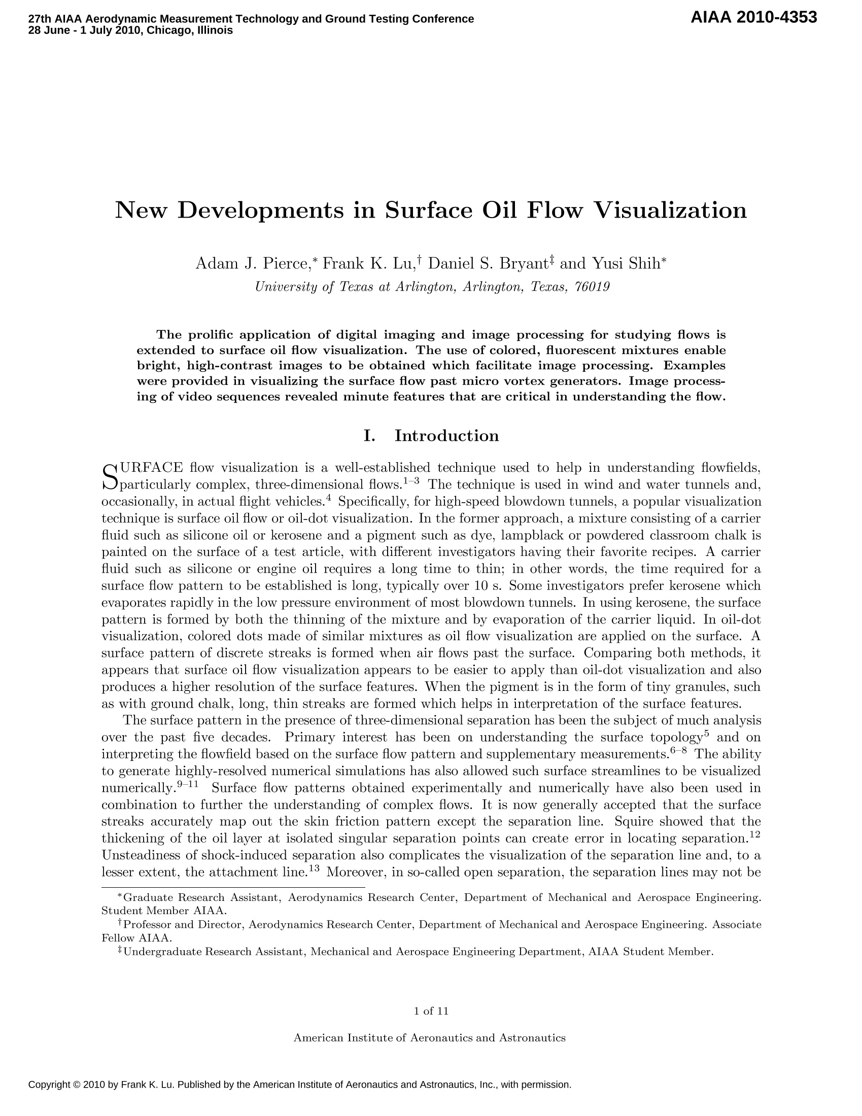
The prolific application of digital imaging and image processing for studying flows is
extended to surface oil flow visualization. The use of colored, fluorescent mixtures enable
bright, high-contrast images to be obtained which facilitate image processing. Examples
were provided in visualizing the surface flow past micro vortex generators. Image processing
of video sequences revealed minute features that are critical in understanding the flow.
方案详情

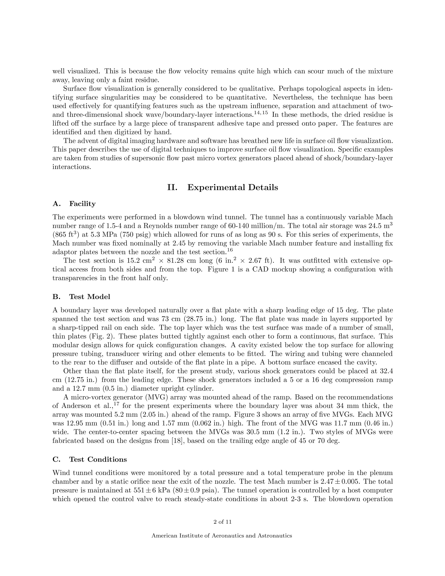
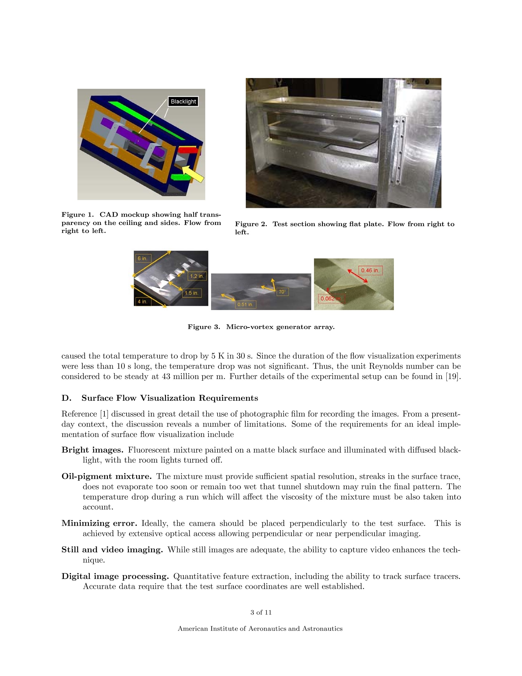
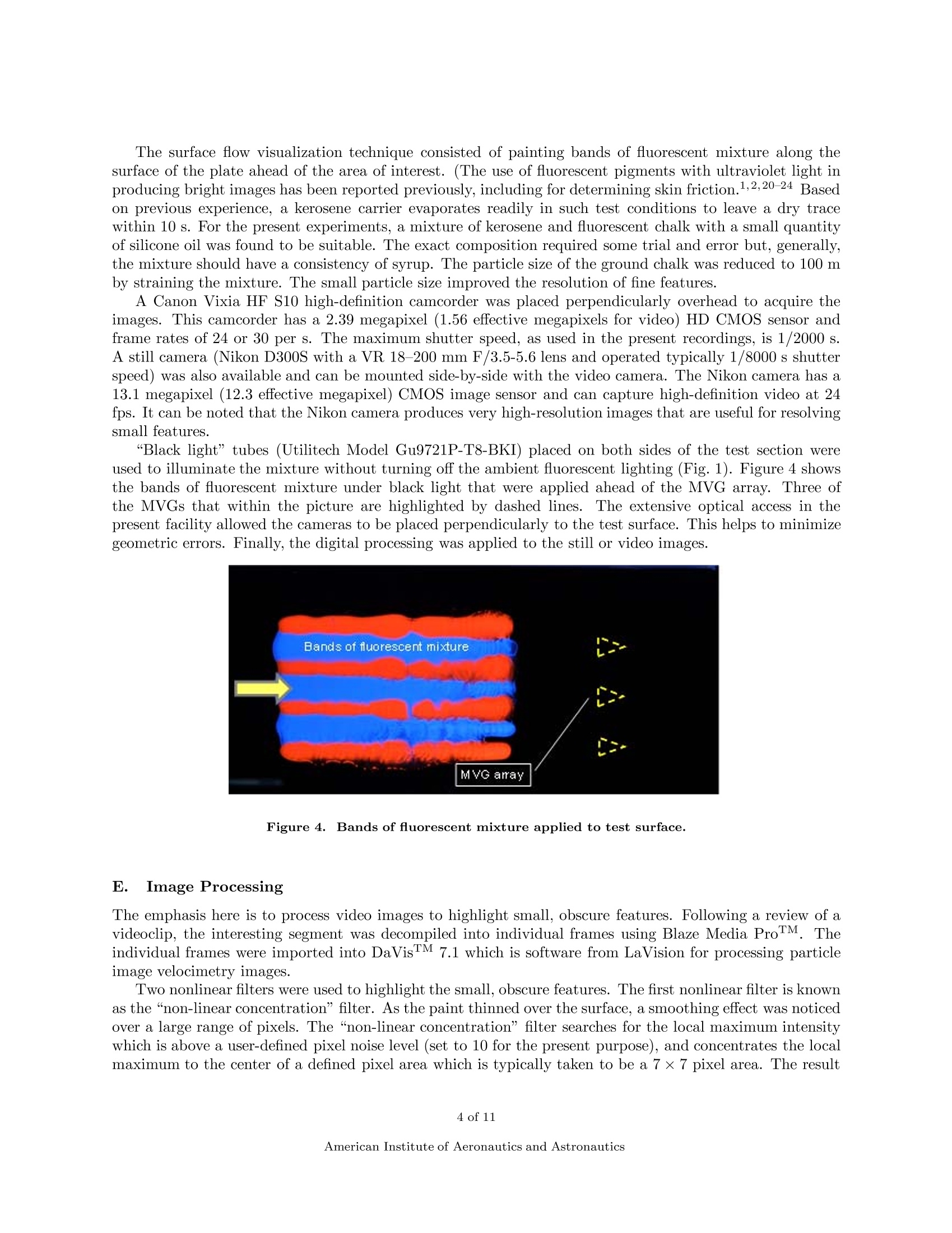
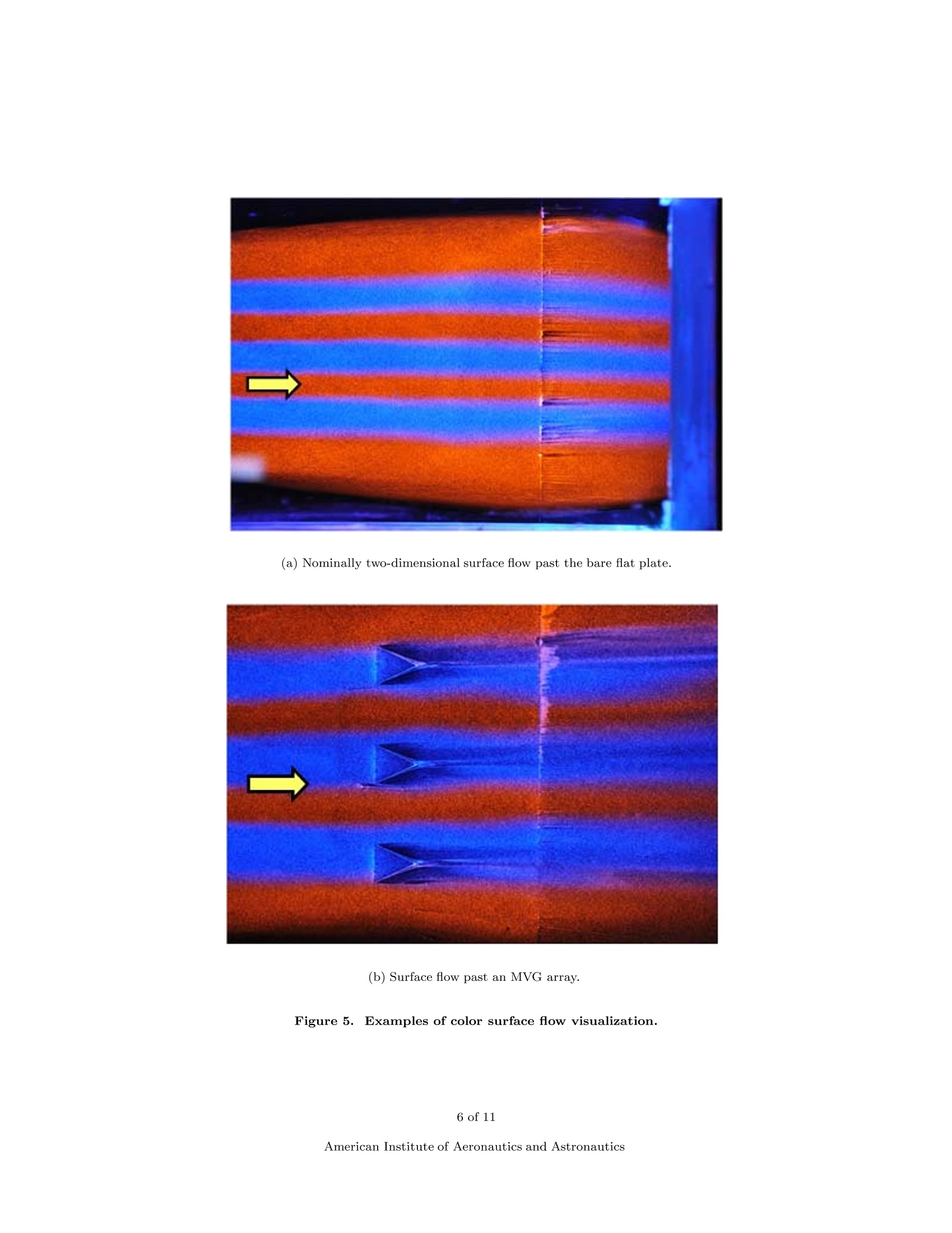
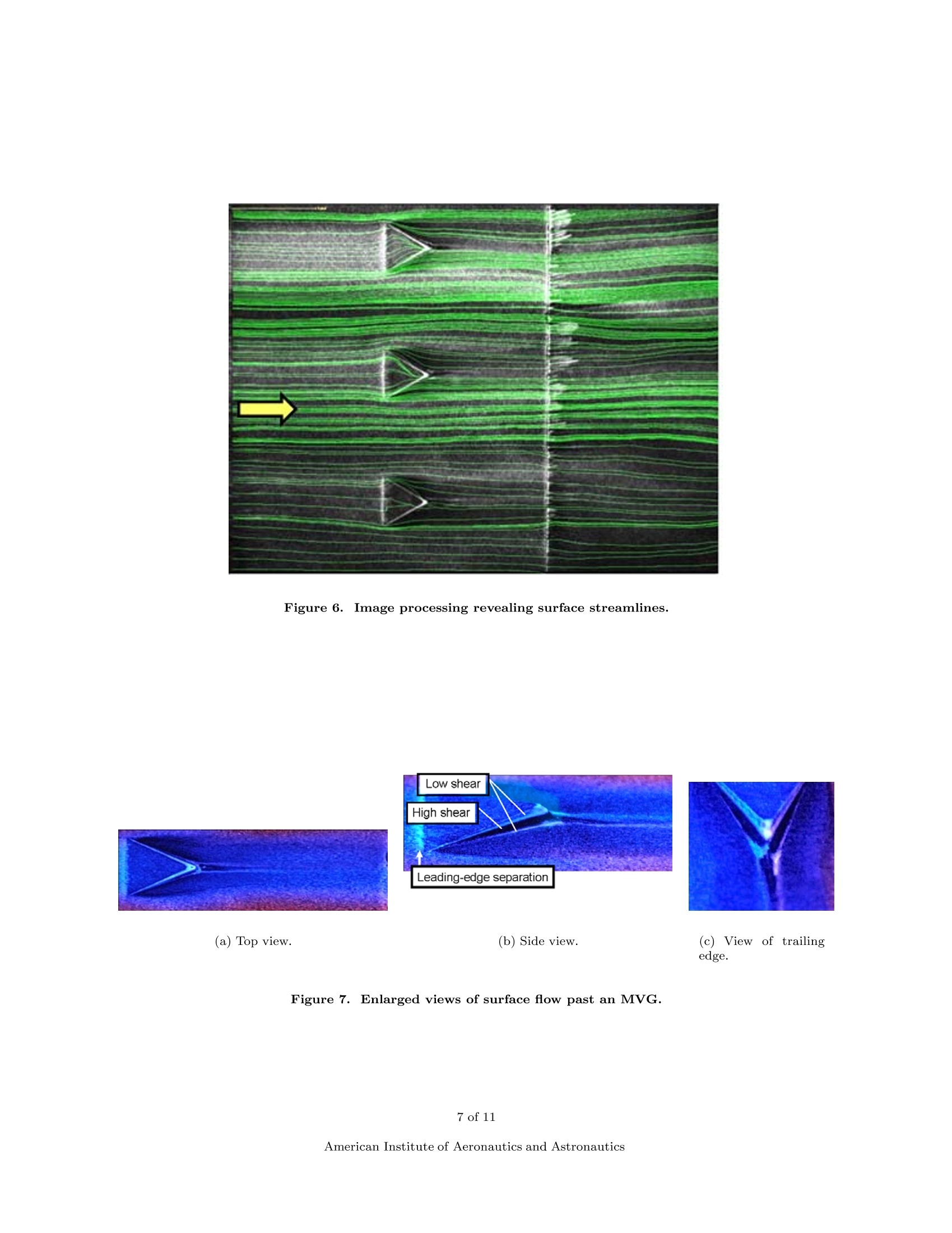
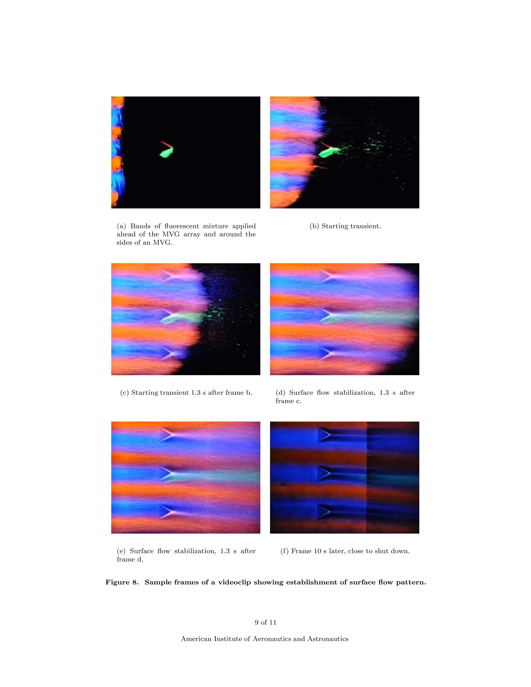
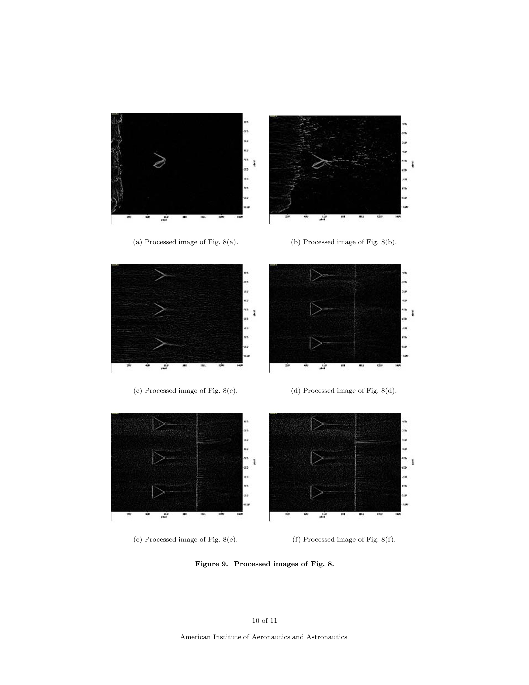
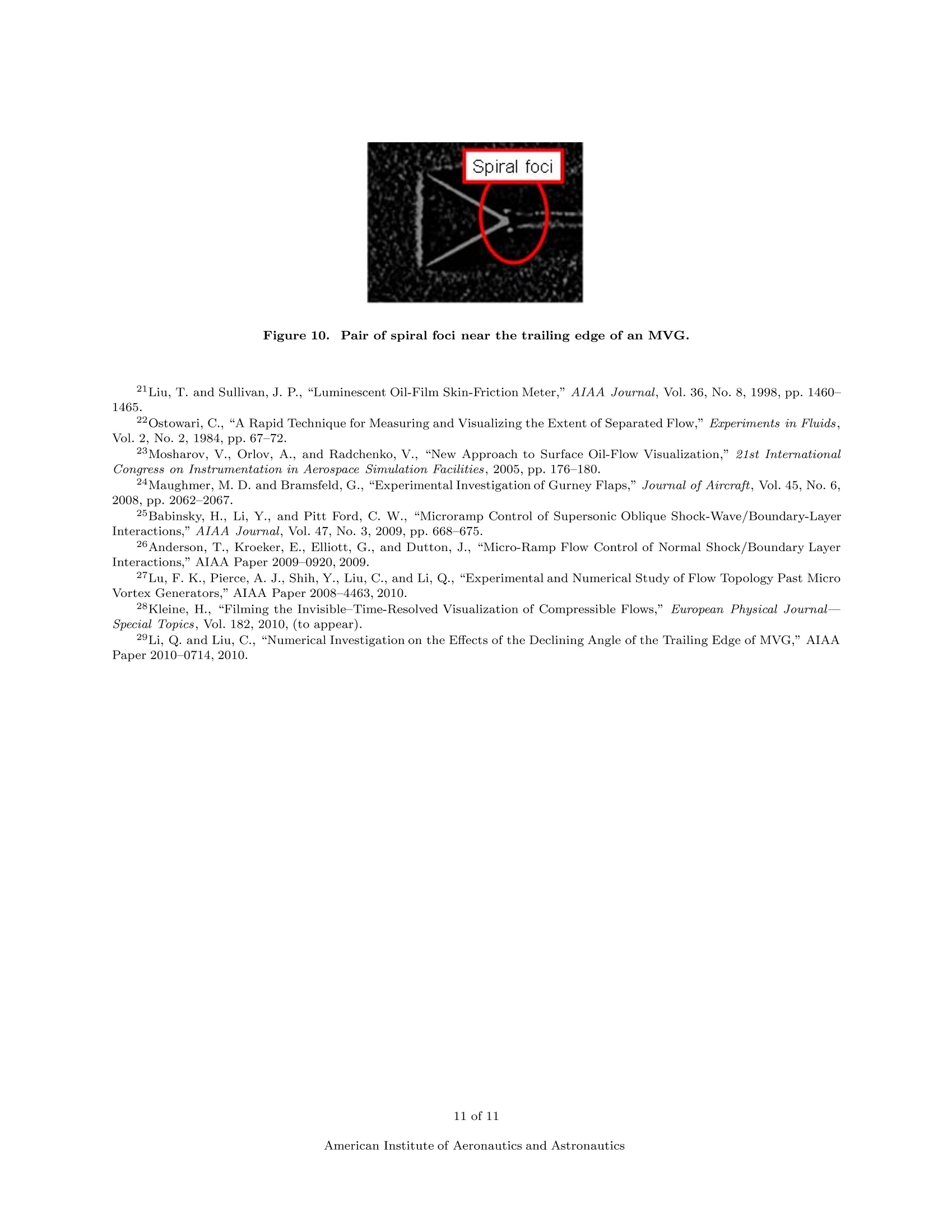
AIAA 2010-435327th AIAA Aerodynamic Measurement Technology and Ground Testing Conference28 June-1 July 2010, Chicago, Illinois New Developments in Surface Oil Flow Visualization Adam J. Pierce,* Frank K. Lu,t Daniel S. Bryant and Yusi Shih* University of Tesas at Arlington, Arlington, Texas, 76019 The prolific application of digital imaging and image processing for studying flows isextended to surface oil flow visualization. The use of colored, fluorescent mixtures enablebright, high-contrast images to be obtained which facilitate image processing.Exampleswere provided in visualizing the surface flow past micro vortex generators. Image process-ing of video sequences revealed minute features that are critical in understanding the flow. I. Introduction URFACE flow visualization is a well-established technique used to help in understanding flowfields,particularly complex, three-dimensional flows.1-3 The technique is used in wind and water tunnels and,occasionally, in actual flight vehicles.4 Specifically, for high-speed blowdown tunnels, a popular visualizationtechnique is surface oil flow or oil-dot visualization. In the former approach, a mixture consisting of a carrierfluid such as silicone oil or kerosene and a pigment such as dye, lampblack or powdered classroom chalk ispainted on the surface of a test article, with different investigators having their favorite recipes. A carrierfluid such as silicone or engine oil requires a long time to thin; in other words, the time required for asurface flow pattern to be established is long, typically over 10 s. Some investigators prefer kerosene whichevaporates rapidly in the low pressure environment of most blowdown tunnels. In using kerosene, the surfacepattern is formed by both the thinning of the mixture and by evaporation of the carrier liquid. In oil-dotvisualization, colored dots made of similar mixtures as oil flow visualization are applied on the surface. Asurface pattern of discrete streaks is formed when air flows past the surface. Comparing both methods, itappears that surface oil flow visualization appears to be easier to apply than oil-dot visualization and alsoproduces a higher resolution of the surface features. When the pigment is in the form of tiny granules, suchas with ground chalk, long, thin streaks are formed which helps in interpretation of the surface features. The surface pattern in the presence of three-dimensional separation has been the subject of much analysisover the past five decades..Primary interest has been on understanding the surface topology and oninterpreting the flowfield based on the surface flow pattern and supplementary measurements.6-8 The abilityto generate highly-resolved numerical simulations has also allowed such surface streamlines to be visualizednumerically.9-11Surface flow patterns obtained experimentally and numerically have also been used incombination to further the understanding of complex flows. It is now generally accepted that the surfacestreaks accurately map out the skin friction pattern except the separation line. Squire showed that thethickening of the oil layer at isolated singular separation points can create error in locating separation.Unsteadiness of shock-induced separation also complicates the visualization of the separation line and, to alesser extent, the attachment line.13 Moreover, in so-called open separation, the separation lines may not be ( *Graduate Research Assistant , Aerodynamics Research Center, D epartment of Mechanical and A e rospace Engineering. Student Member AIAA. ) ( T Professor a nd Direct o r, A erodynamics Research Center, Depar t ment of Mecha n ical and A erospace Engineering. Associate Fellow AIAA. ) ( +Undergraduate Research Assistant, M echanical and Aerospace E n gineering Department,AIAA Stud e nt Memb e r. ) well visualized. This is because the flow velocity remains quite high which can scour much of the mixtureaway, leaving only a faint residue. Surface flow visualization is generally considered to be qualitative. Perhaps topological aspects in iden-tifying surface singularities may be considered to be quantitative. Nevertheless, the technique has beenused effectively for quantifying features such as the upstream influence, separation and attachment oftwo-and three-dimensional shock wave/boundary-layer interactions.14,15In these methods, the dried residue islifted off the surface by a large piece of transparent adhesive tape and pressed onto paper. The features areidentified and then digitized by hand. The advent of digital imaging hardware and software has breathed new life in surface oil flow visualization.This paper describes the use of digital techniques to improve surface oil flow visualization. Specific examplesare taken from studies of supersonic flow past micro vortex generators placed ahead of shock/boundary-layerinteractions. II. Experimental Details A. Facility The experiments were performed in a blowdown wind tunnel. The tunnel has a continuously variable Machnumber range of 1.5-4 and a Reynolds number range of 60-140 million m. The total air storage was 24.5 m(865 ft) at 5.3 MPa (750 psig) which allowed for runs of as long as 90 s. For this series of experiments, theMach number was fixed nominally at 2.45 by removing the variable Mach number feature and installing fixadaptor plates between the nozzle and the test section.16 The test section is 15.2 cm² × 81.28 cm long (6 in.2× 2.67 ft). It was outfitted with extensive op-tical access from both sides and from the top. Figure 1 is a CAD mockup showing a configuration withtransparencies in the front half only. B. Test Model A boundary layer was developed naturally over a flat plate with a sharp leading edge of 15 deg. The platespanned the test section and was 73 cm (28.75 in.) long. The flat plate was made in layers supported bya sharp-tipped rail on each side. The top layer which was the test surface was made of a number of small,thin plates (Fig.2). These plates butted tightly against each other to form a continuous, flat surface. Thismodular design allows for quick configuration changes. A cavity existed below the top surface for allowingpressure tubing, transducer wiring and other elements to be fitted. The wiring and tubing were channeledto the rear to the diffuser and outside of the flat plate in a pipe. A bottom surface encased the cavity. Other than the flat plate itself, for the present study, various shock generators could be placed at 32.4cm (12.75 in.) from the leading edge. These shock generators included a 5 or a 16 deg compression rampand a 12.7 mm (0.5 in.) diameter upright cylinder. A micro-vortex generator (MVG) array was mounted ahead of the ramp. Based on the recommendationsof Anderson et al.,for the present experiments where the boundary layer was about 34 mm thick, thearray was mounted 5.2 mm (2.05 in.) ahead of the ramp. Figure 3 shows an array of five MVGs. Each MVGwas 12.95 mm (0.51 in.) long and 1.57 mm (0.062 in.) high. The front of the MVG was 11.7 mm (0.46 in.)wide. The center-to-center spacing between the MVGs was 30.5 mm (1.2 in.). Two styles of MVGs werefabricated based on the designs from [18], based on the trailing edge angle of 45 or 70 deg. C..Test Conditions Wind tunnel conditions were monitored by a total pressure and a total temperature probe in the plenumchamber and by a static orifice near the exit of the nozzle. The test Mach number is 2.47±0.005. The totalpressure is maintained at 551±6 kPa (80±0.9 psia). The tunnel operation is controlled by a host computerwhich opened the control valve to reach steady-state conditions in about 2-3 s.The blowdown operation Figure 1. CAD mockup showing half trans-parency on the ceiling and sides. Flow fromright to left. Figure 2. Test section showing flat plate. Flow from right toleft. Figure 3. MNicro-vortex generator array. caused the total temperature to drop by 5K in 30 s. Since the duration of the flow visualization experimentswere less than 10 s long, the temperature drop was not significant. Thus, the unit Reynolds number can beconsidered to be steady at 43 million per m. Further details of the experimental setup can be found in [19]. D).Surface Flow Visualization Requirements Reference [1] discussed in great detail the use of photographic film for recording the images. From a present-day context, the discussion reveals a number of limitations. Some of the requirements for an ideal imple-mentation of surface flow visualization include Bright images. Fluorescent mixture painted on a matte black surface and illuminated with diffused black-light, with the room lights turned off. Oil-pigment mixture. The mixture must provide sufficient spatial resolution, streaks in the surface trace,does not evaporate too soon or remain too wet that tunnel shutdown may ruin the final pattern. Thetemperature drop during a run which will affect the viscosity of the mixture must be also taken intoaccount. Minimizing error. Ideally, the camera should be placed perpendicularly to the test surface.This isachieved by extensive optical access allowing perpendicular or near perpendicular imaging. Still and video imaging. While still images are adequate, the ability to capture video enhances the tech-nique. Digital image processing. Quantitative feature extraction, including the ability to track surface tracers.Accurate data require that the test surface coordinates are well established. The surface flow visualization technique consisted of painting bands of fluorescent mixture along thesurface of the plate ahead of the area of interest. (The use of fluorescent pigments with ultraviolet light inproducing bright images has been reported previously, including for determining skin friction. 1,2,20-24 Basedon previous experience, a kerosene carrier evaporates readily in such test conditions to leave a dry tracewithin 10 s. For the present experiments, a mixture of kerosene and fluorescent chalk with a small quantityof silicone oil was found to be suitable. The exact composition required some trial and error but, generally,the mixture should have a consistency of syrup. The particle size of the ground chalk was reduced to 100 mby straining the mixture. The small particle size improved the resolution of fine features. A Canon Vixia HF S10 high-definition camcorder was placed perpendicularly overhead to acquire theimages. This camcorder has a 2.39 megapixel (1.56 effective megapixels for video) HD CMOS sensor andframe rates of 24 or 30 per s. The maximum shutter speed, as used in the present recordings, is 1/2000 s.A still camera (Nikon D300S with a VR 18-200 mm F/3.5-5.6 lens and operated typically 1/8000 s shutterspeed) was also available and can be mounted side-by-side with the video camera. The Nikon camera has a13.1 megapixel (12.3 effective megapixel) CMOS image sensor and can capture high-definition video at 24fps. It can be noted that the Nikon camera produces very high-resolution images that are useful for resolvingsmall features. “Black light" tubes (Utilitech Model Gu9721P-T8-BKI) placed on both sides of the test section wereused to illuminate the mixture without turning off the ambient fluorescent lighting (Fig. 1). Figure 4 showsthe bands of fluorescent mixture under black light that were applied ahead of the MVG array.Three ofthe MVGs that within the picture are highlighted by dashed lines.S.TThe extensive optical access in thepresent facility allowed the cameras to be placed perpendicularly to the test surface. This helps to minimizegeometric errors. Finally, the digital processing was applied to the still or video images. Figure 4. Bands of fluorescent mixture applied to test surface. E.]Image Processing The emphasis here is to process video images to highlight small, obscure features. Following a review of avideoclip, the interesting segment was decompiled into individual frames using Blaze Media ProM. Theindividual frames were imported into DaVisTM 7.1 which is software from LaVision for processing particleimage velocimetry images. Two nonlinear filters were used to highlight the small, obscure features. The first nonlinear filter is knownas the “non-linear concentration”filter. As the paint thinned over the surface, a smoothing effect was noticedover a large range of pixels. The “non-linear concentration” filter searches for the local maximum intensitywhich is above a user-defined pixel noise level (set to 10 for the present purpose), and concentrates the localmaximum to the center of a defined pixel area which is typically taken to be a 7×7 pixel area. The result of this operation is to convert the color image into a high-contrast gray scale image. The second non-linearfilter applied is the “non-linear subtraction sliding minimum”filter. This filter computes the local minimumover a user defined scale pixel length. This filter was chosen to further increase the contrast, whereby localmaxima of intensity are made visible. Due to the precious concentration filtering process, this second processresults in a pure black-and-white image, with no gray. After the image processing was completed, the imageswere recompiled into a video clip using Blaze Media ProTM. III. Results and Discussion An example of the surface flow past the bare flat plate and the MVG array is shown in Fig. 5. Figure5(a) shows that the surface flow past the bare flat plate is mostly two-dimensional. Departures from two-dimensionality at the top and bottom of the figure are due to the way the mixture was applied. A similarremark can be made of the flow past the MVG array. One of the image processing techniques is simply to use normal PIV vector calculations on the surfaceflow, treating the surface flow as if it consists of particles convecting downstream. This yielded a “surfacestreamline”map shown as green lines in Fig. 6. The map is superimposed on the original surface visualization,now shown in gray scale. It is clear that the surface streamlines are visualized well. There should not be anyinference on surface velocity, however. While not attempted presently, it should be possible to quantify thetwo-dimensionality of the surface flow instead of merely suggesting that the surface flow is two dimensionalvisually. Next, enlargements showing the details around an MVG are found in Fig. 7. The top view in Fig. 7(a)shows bright regions, indicating an accumulation of mixture, telltale signs that these are regions of low shear.The accumulation at the leading edge of the MVG can be readily interpreted as a region of two-dimensionalseparation. The fluid in the separation zone leaves from the sides, rolling up into so-called horseshoe vortices.These are regions of high shear which manifest themselves as darker regions, with the pigment being scouredaway, as also observed by others.25,26 Figure 7(a) also shows accumulation on the side edges of the MVG and in a pair of long streaks on the flatplate behind the MVG. These require careful interpretation but cannot be achieved with the view directlyoverhead. Instead, the side view of Fig.7(b) shows that there are in fact two regions of low shear on theside, one near the top edge of the MVG and the other at the junction of the MVG with the flat plate; seealso [25-27]. These low shear regions are separated by a region that appears devoid of pigment, indicating aregion of extremely high shear. Thus, a more complex topology is now revealed that was not evident fromthe overhead view. To assist in identifying the type of separation around the MVG, a differently colored pigment was appliedon the flat plate adjacent to the slant surfaces as shown in Fig. 8(a) of a sequence of frames from a videoclip.The sequence shows that the mixture around the slant surfaces is blown away. This indicates a high-speedregion associated with open separation. Kleine28 suggests that videos enable changes to be studied. Thus,visualizing the start-up transient of the surface flow in this manner can help to understand the complex flow. In addition, Kleine28 suggests that minute features can be identified in a video that may otherwise beconsidered to be erroneous in a single image. In the present case, the videoclip is processed as describedpreviously and some of the frames are shown in Fig. 9. Even though the present video is not time resolved,playing the video allows a minute but critical feature to be identified. A careful examination of Fig. 9 revealsthe presence of a pair of foci which corroborates numerical evidence;9see Fig. 10 For a more detaileddiscussion, see [27]. IV. Conclusions The implementation of digital imaging and image processing has revitalized surface flow visualization.The implementations were illustrated using micro vortex generators in a supersonic flow. A technique for (a) Nominally two-dimensional surface flow past the bare flat plate. (b) Surface flow past an MVG array. Figure 5. Examples of color surface flow visualization. Figure 6. IImage processing revealing surface streamlines. Figure 7. Enlarged views of surface flow past an MVG. obtaining bright surface visualizations using fluorescent chalk was described. The images were captured byeither a still or a video camera. Although the videos were not time resolved, the animated sequences allowedfor the detection of minute but critical features in the surface flow which can be connected topologically tothe entire flowfield. Acknowledgments The authors gratefully acknowledge funding for this work via AFOSR Grant No. FA9550-08-1-0201monitored by Dr. John Schmisseur. Daniel Bryant was supported by the Dean’s Undergraduate ResearchApprenticeship from the College of Engineering. The authors thank the assistance of Rod Duke and DavidWhaley with the experiments. David Whaley was supported by a High School Research Internship undera Texas Youth in Technology grant, administered by Dr. J. Carter M. Tiernan, Assistant Dean for StudentAffairs in the College of Engineering, University of Texas at Arlington. References -Maltby, R. L.,“Flow Visualization in Wind Tunnels Using Indicators,”AGARDograph 70, 1962. Merzkirch, W., Flow Visualization, Academic, Orlando, Florida, 2nd ed., 1987. Lu,F. K., “Surface Flow Visualization: Still Useful After All These Years,”European Physical Journal—Special Topics,Vol. 182,2010, (to appear). 4Meyer, R. R. and Jennett, L. A.,“In-Flight Surface Oil-Flow Photographs with Comparisons to Pressure Distributionand Boundary-Layer Data," NASA TP 2395, 1985. Tobak, M. and Peake, D. J.,“Topology of Three-Dimensional Separated Flows,” Annual Review of Fluid Mechanics,Vol. 14, 1982, pp. 61-85. Perry, A. E. and Chong, M. S.,“A Description of Eddying Motions and Flow Patterns Using Critical-Point Concepts,”Annual Review ofFluid Mechanics, Vol. 19, 1987, pp. 125-155. Chapman, G. T. and Yates, L. A.,“Topology of Flow Separation on Three-Dimensional Bodies,” Applied MechanicsReview, Vol. 44, No. 7, 1991,pp. 329-345. Depardon,S., J. J., Lasserre, Brizzi, L. E., and Bor’ee, J.,“Automated Topology Classification Method for InstantaneousVelocity Fields,” Experiments in Fluids, Vol. 42, No. 5, 2007, pp.697-710. Kenwright, D. N., Henze, C., and Levit, C.,“Feature Extraction of Separation and Attachment Lines,” IEEE Transactionson Visualization and Computer Graphics, Vol. 5, No.2,1999,pp.135-144. 10Venkata, S. D., Jiang, M., Thompson, D. S., and Machiraju, R.,“Automated Detection of Vortex Cores and SeparatedFlows in CFD Datasets,” Proceedings of the 8th International Conference on Numerical Grid Generation in ComputationalField Simulations, Honolulu, Hawaii,2002, pp. 529-538. Mahrous, K. M., Bennett, J. C., Hamann, B., and Joy, K. I.,“Improving Topological Segmentation of Three-DimensionalVector Fields,” Joint EUROGRAPHICS-IEEE TCVG Symposium on Visualization, edited by G.-P. Bonneau, S. Hahmann,and C. D. Hansen, 2003. 12Squire, L. C., “The Motion of a Thin Oil Sheet Under the Steady Boundary Layer on a Body,”Journal of Fluid Mechanics,Vol. 11, No. 2, 1961,pp. 161-179. 13Gramann, R. A. and Dolling, D. S., “Interpretation of Separation Lines from Surface Tracers in a Shock-InducedTurbulent-Flow,”AIAA Journal, Vol. 25, No. 12,1987, pp. 1545-1546. 14Settles, G. S. and Teng, H. Y., “Flow Visualization Methods for Separated 3-Dimensional Shock-Wave TurbulentBoundary-Layer Interactions,”AIAA Journal, Vol. 21, No. 3, 1983, pp. 390-397. 15Lu, F. K., “Color Surface-Flow Visualization of Fin-Generated Shock-Wave Boundary-Layer Interactions,”Experimentsin Fluids, Vol. 8, No. 6, 1990, pp. 352-354. 16Mitchell, R. R. and Lu, F. K., “Development of a Supersonic Aerodynamic Test Section using Computational Modeling,”AIAA Paper 2009-3573,2009. 17 Anderson, B. H. Tinapple,J., and Sorber, L.,“Optimal Control of Shock Wave Turbulent Boundary Layer InteractionsUsing Micro-Array Actuation,"AIAA Paper 2006-3197,2006. 18Li, Q. and Liu, C., “LES for Supersonic Ramp Control Flow Using MVG at M= 2.5 and Reg = 1440,”AIAA Paper2010-0592,2010. 19Pierce, A. J., Experimental Study of Micro-Vorter Generators at Mach 2.5, MSAE thesis, University of Texas at Arling-ton, 2010. 20Loving, D. L. and Katzoff, S.,“The Fluorescent-Oil Film Method and Other Techniques for Boundary-Layer FlowVisualization,”NASA Memo 3-17-59L,1959. (a) Bands of fluorescent mixture appliedahead of the MVG array and around thesides of an MVG. (b) Starting transient. (c) Starting transient 1.3 s after frame b. (d) Surface flow stabilization, 1.3 s afterframe c. (e) Surface flow stabilization, 1.3 s afterframe d. (f) Frame 10 s later, close to shut down. Figure 8.. SSample frames of a videoclip showing establishment of surface flow pattern. (a) Processed image of Fig. 8(a). (b) Processed image of Fig. 8(b). (e) Processed image of Fig. 8(e). (f) Processed image of Fig.8(f). Figure 9. Processed images of Fig. 8. Figure 10. Pair of spiral foci near the trailing edge of an MVG. 2Liu, T. and Sullivan,J. P., “Luminescent Oil-Film Skin-Friction Meter,”AIAA Journal, Vol. 36, No. 8, 1998, pp. 1460-1465. 22Ostowari, C.,“A Rapid Technique for Measuring and Visualizing the Extent of Separated Flow,” Experiments in Fluids,Vol. 2, No. 2, 1984, pp. 67-72. 23Mosharov, V., Orlov, A., and Radchenko,V., “New Approach to Surface Oil-Flow Visualization,”21st InternationalCongress on Instrumentation in Aerospace Simulation Facilities,2005, pp.176-180. 24Maughmer, M. D. and Bramsfeld, G.,“Experimental Investigation of Gurney Flaps,” Journal of Aircraft, Vol. 45, No. 6,2008,pp. 2062-2067. 25Babinsky, H., Li, Y., and Pitt Ford, C.W.,“Microramp Control of Supersonic Oblique Shock-Wave/Boundary-LayerInteractions,”AIAA Journal,Vol. 47, No. 3, 2009, pp.668-675. 26Anderson, T., Kroeker, E., Elliott, G.,and Dutton,J.,“Micro-Ramp Flow Control of Normal Shock/Boundary LayerInteractions,"AIAA Paper2009-0920,2009. 27Lu, F. K., Pierce, A. J., Shih, Y., Liu, C., and Li, Q.,“Experimental and Numerical Study of Flow Topology Past MicroVortex Generators,"AIAA Paper 2008-4463,2010. 28Kleine, H.,“Filming the Invisible-Time-Resolved Visualization of Compressible Flows,” European Physical Journal-Special Topics, Vol. 182, 2010, (to appear). 29Li, Q.and Liu, C.,“Numerical Investigation on the Effects of the Declining Angle of the Trailing Edge ofMVG,"AIAAPaper 2010-0714,2010. of merican Institute of Aeronautics and AstronauticsCopyright C by Frank K. Lu. Published by the American Institute of Aeronautics and Astronautics, Inc., with permission. of merican Institute of Aeronautics and Astronautics
确定
还剩9页未读,是否继续阅读?

产品配置单

北京欧兰科技发展有限公司为您提供《油表面流动中速度场检测方案(粒子图像测速)》,该方案主要用于其他中速度场检测,参考标准--,《油表面流动中速度场检测方案(粒子图像测速)》用到的仪器有德国LaVision PIV/PLIF粒子成像测速场仪、Imager SX PIV相机
推荐专场


相关方案
更多
该厂商其他方案
更多