


方案详情
文
Zooplankton feed in either of three ways: they generate a feeding current, cruise through
the water, or they are ambush feeders. Each mode generates different hydrodynamic disturbances
and hence exposes the grazers differently to mechanosensory predators. Ambush feeders sink
slowly and therefore perform occasional upward repositioning jumps. We quantified the fluid
disturbance generated by repositioning jumps in a mm-sized copepod (Re ~ 40). The kick of the
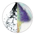
swimming legs generates a viscous vortex ring in the wake; another ring of similar intensity but
opposite rotation is formed around the decelerating copepod. A simple analytical model, that of an
impulsive point force, properly describes the observed flow field as a function of the momentum of
the copepod, including the translation of the vortex and its spatial extension and temporal decay.
We show that the time-averaged fluid signal and the consequent predation risk is much less for an
ambush feeding than a cruising or hovering copepod for small individuals, while the reverse is true
for individuals larger than about 1 mm. This makes inefficient ambush feeding feasible in small
copepods and is consistent with the observation that ambush feeding copepods in the ocean are all
small, while larger species invariably use hovering or cruising feeding strategies.
方案详情

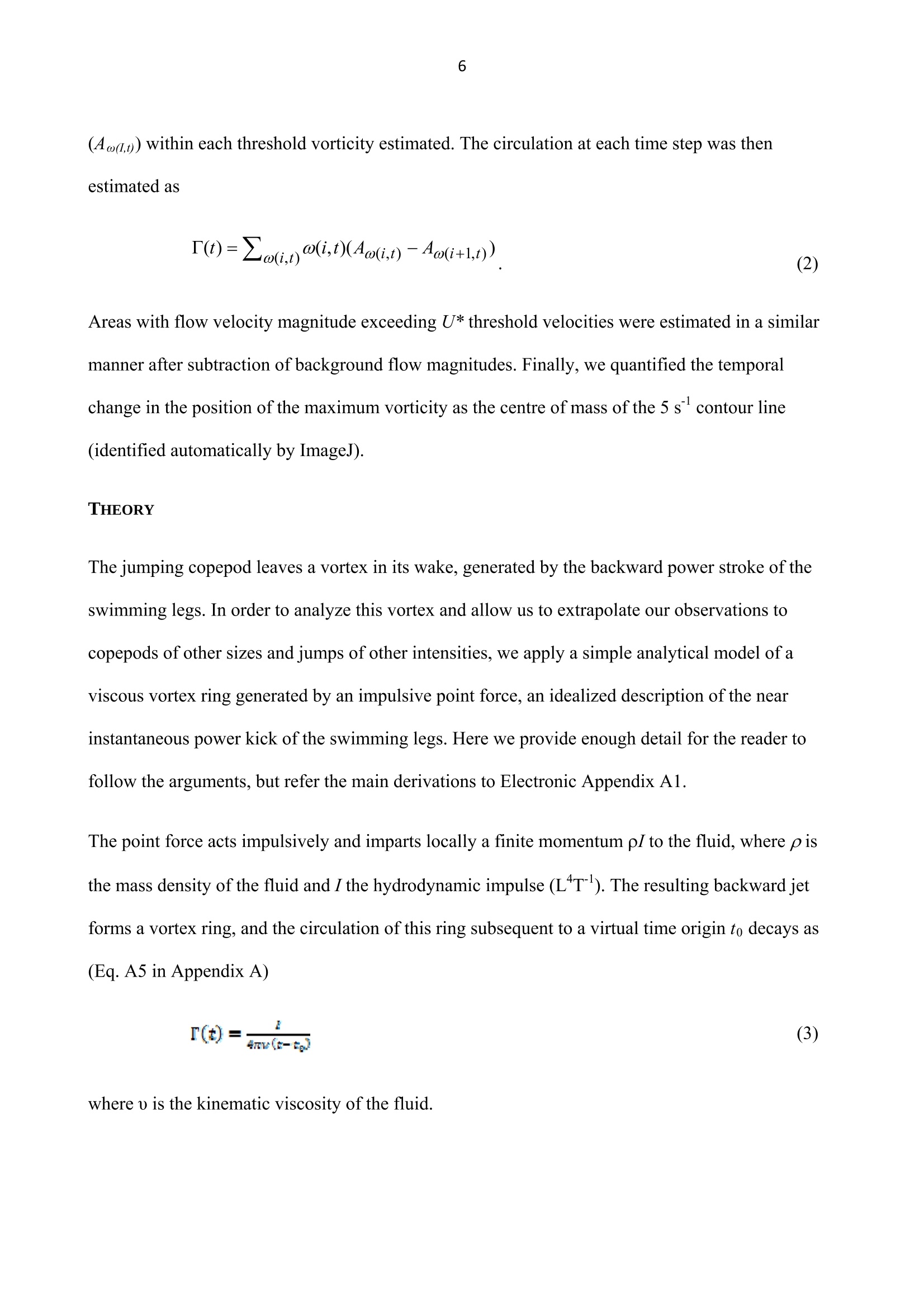
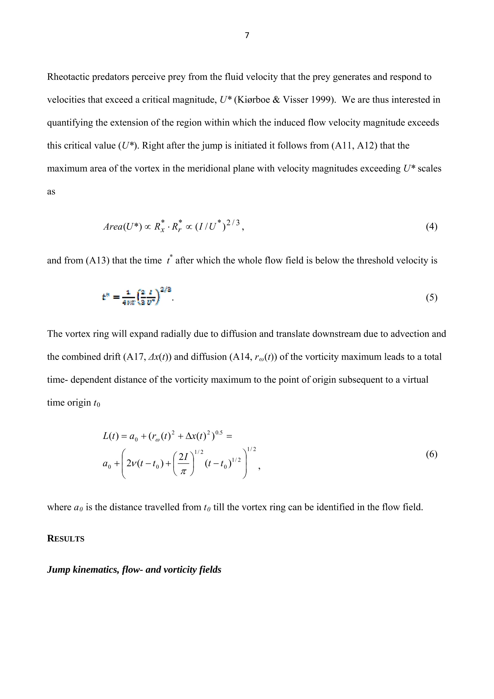
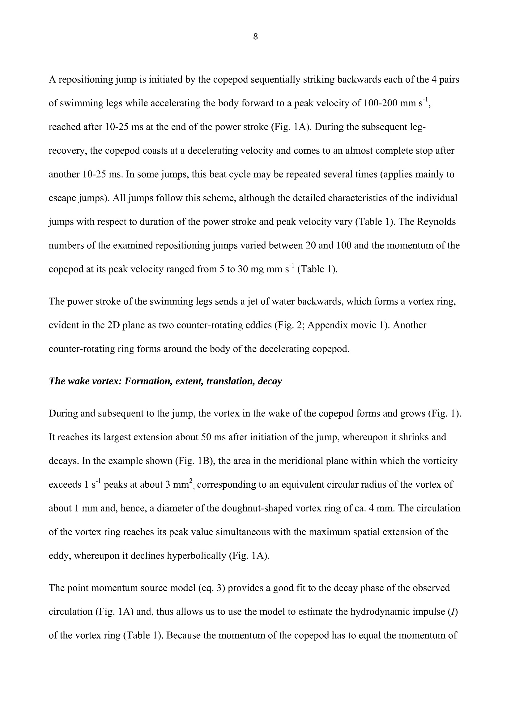
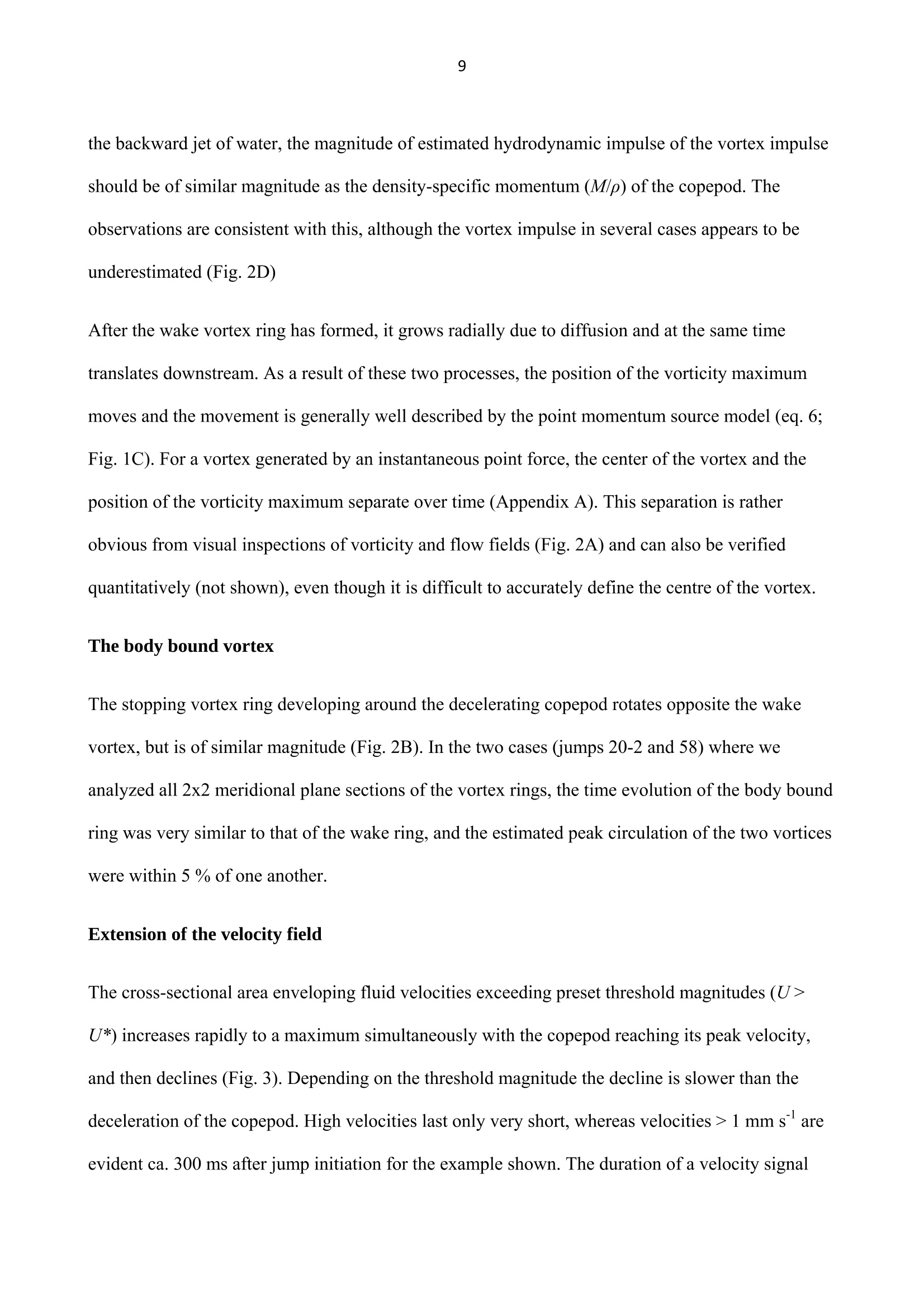
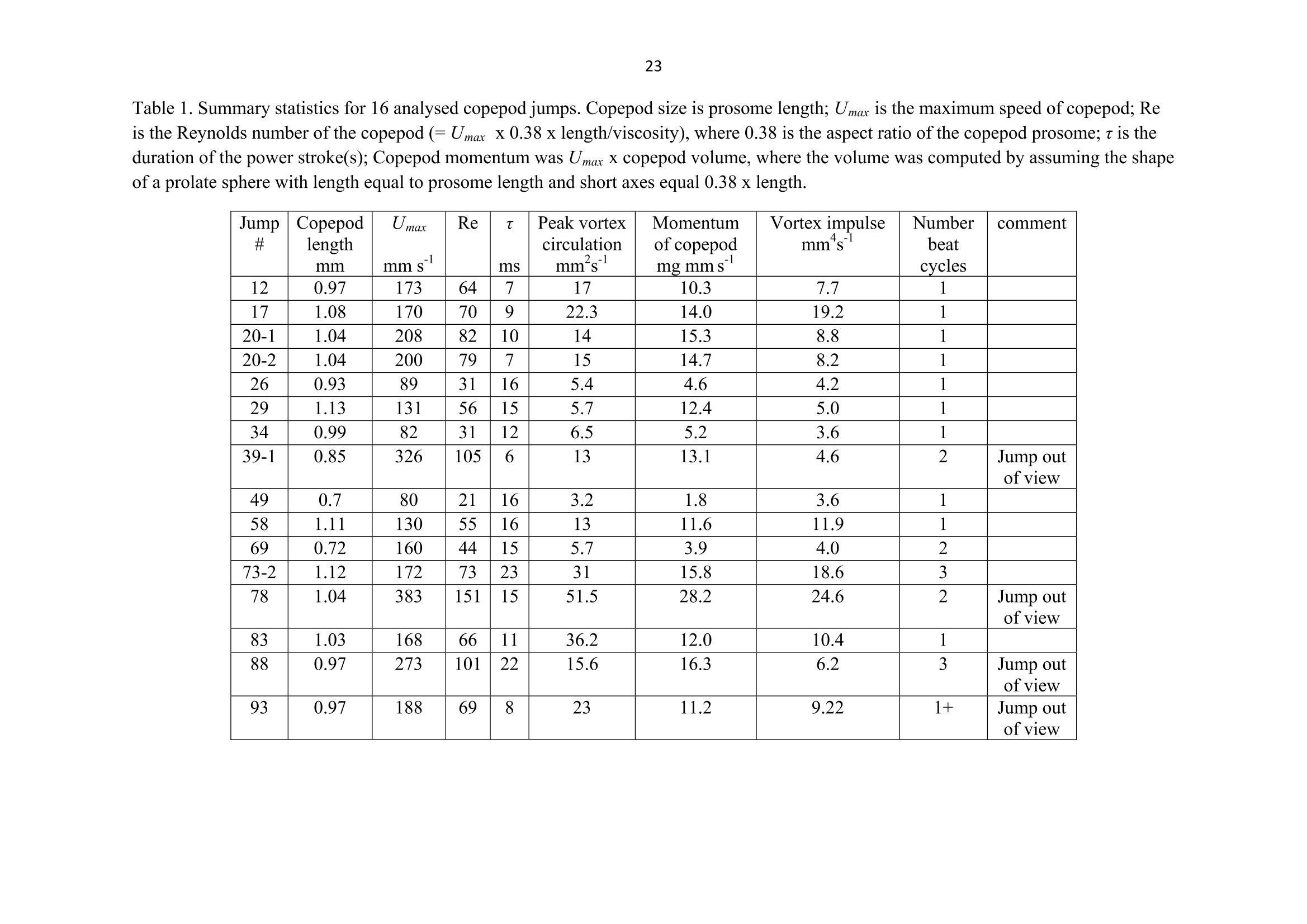
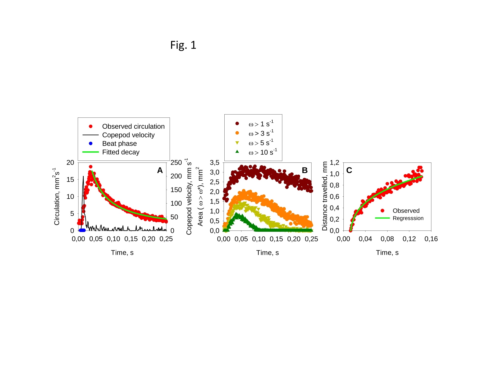
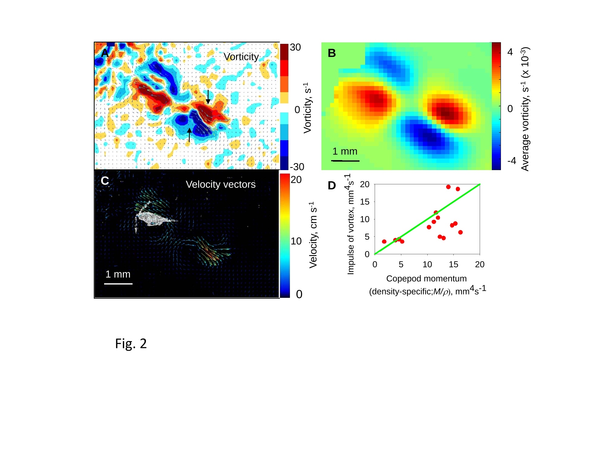
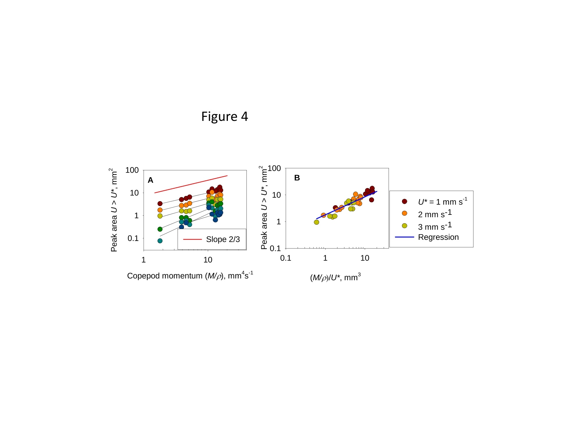
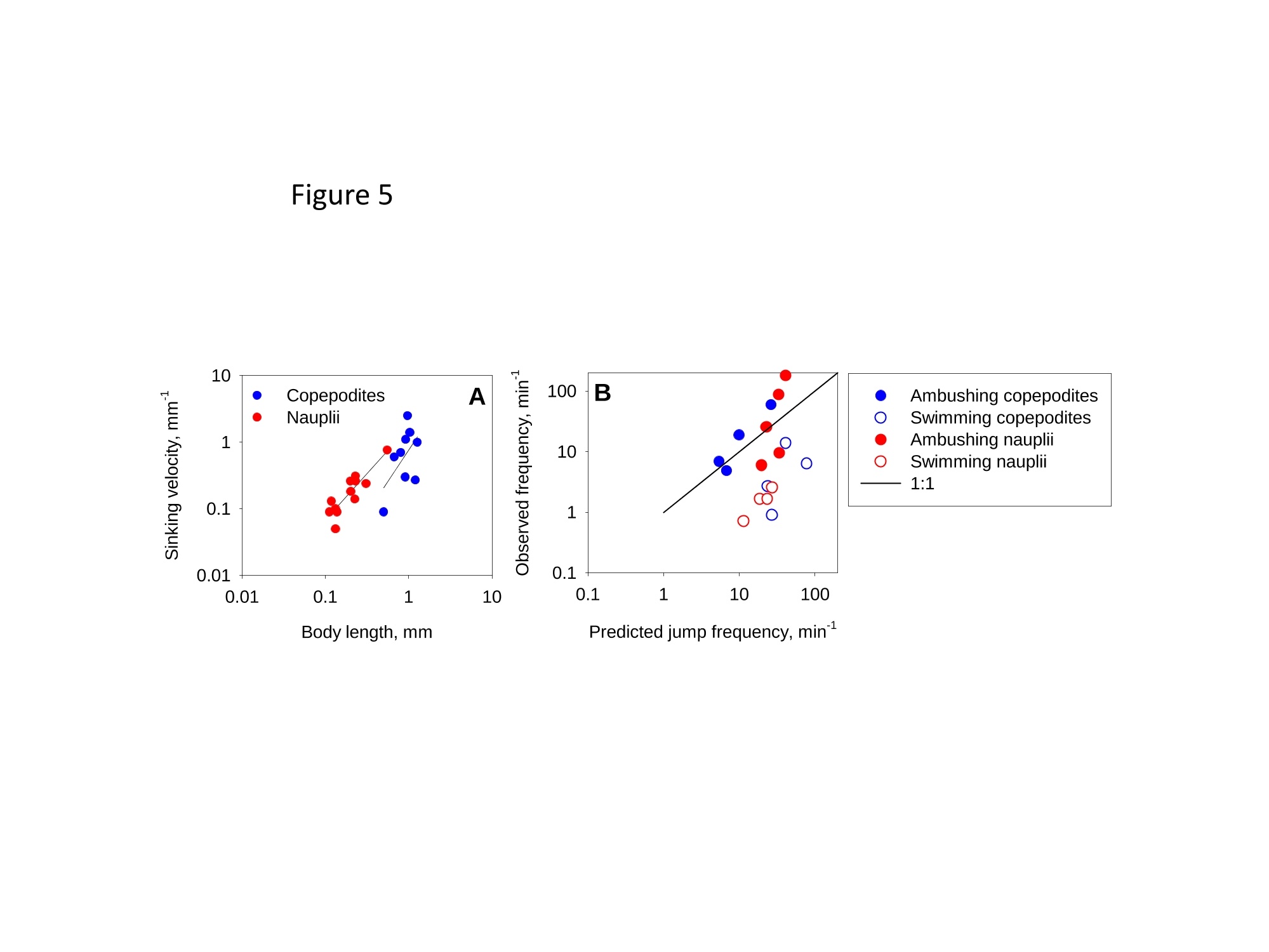
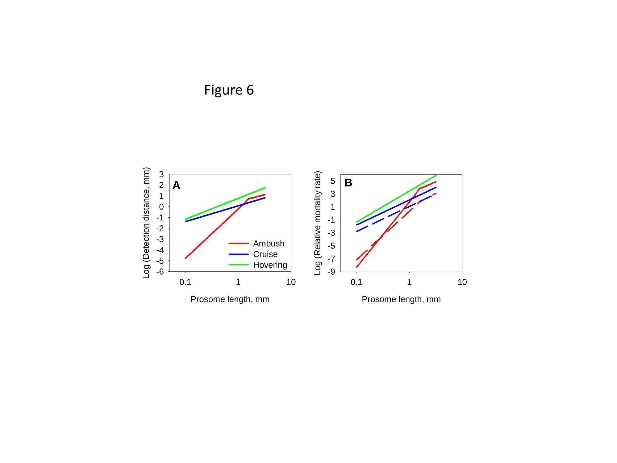
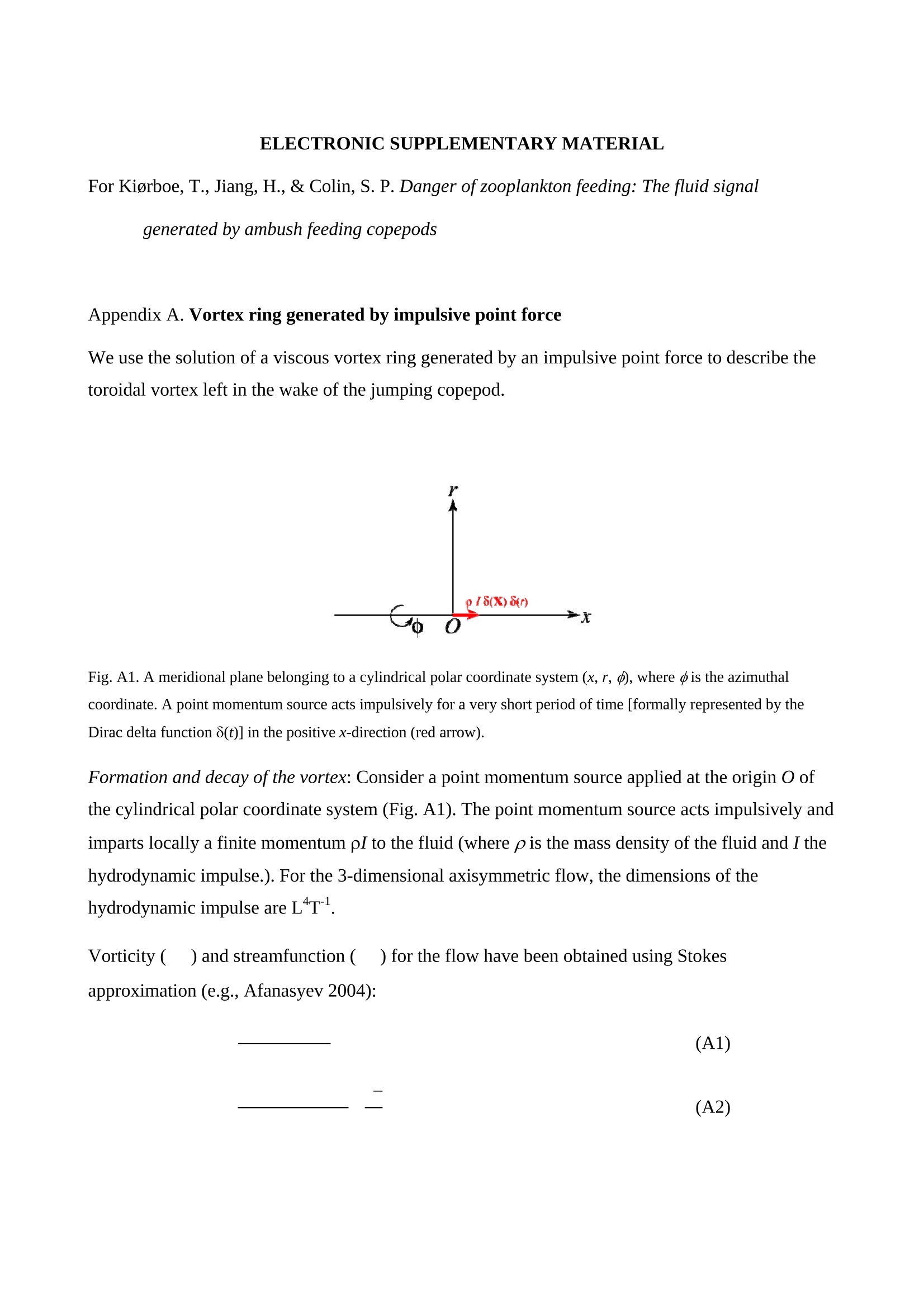
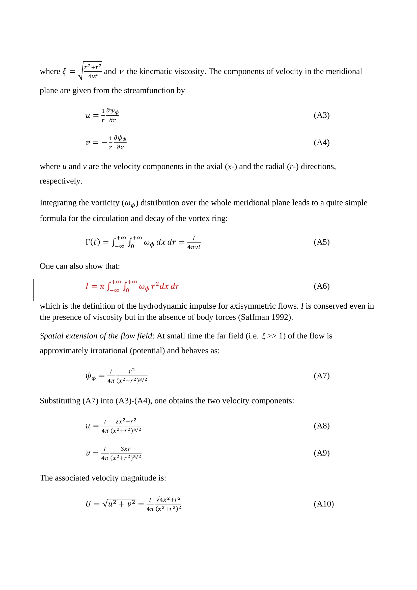
1 2 DANGER OF ZOOPLANKTON FEEDING: THE FLUID SIGNAL GENERATED BY AMBUSH FEEDING COPEPODS Thomas Kiorboe National Institute of Aquatic Resources, Technical University of Denmark, Kavalergarden 6, DK-2920 Charlottenlund,Denmark. Email: tk@aqua.dtu.dk Houshuo Jiang Department of Applied Ocean Physics and Engineering, Woods Hole Oceanographic Institution,Woods Hole, MA 02543, USA Sean P. Colin Environmental Sciences and Marine Biology, Roger Williams University, Bristol, RI 02809, USA Abstract. Zooplankton feed in either of three ways: they generate a feeding current, cruise throughthe water, or they are ambush feeders. Each mode generates different hydrodynamic disturbancesand hence exposes the grazers differently to mechanosensory predators. Ambush feeders sinkslowly and therefore perform occasional upward repositioning jumps. We quantified the fluiddisturbance generated by repositioning jumps in a mm-sized copepod (Re~40). The kick of theswimming legs generates a viscous vortex ring in the wake; another ring of similar intensity butopposite rotation is formed around the decelerating copepod. A simple analytical model, that of animpulsive point force, properly describes the observed flow field as a function of the momentum ofthe copepod, including the translation of the vortex and its spatial extension and temporal decay.We show that the time-averaged fluid signal and the consequent predation risk is much less for anambush feeding than a cruising or hovering copepod for small individuals, while the reverse is truefor individuals larger than about 1 mm. This makes inefficient ambush feeding feasible in smallcopepods and is consistent with the observation that ambush feeding copepods in the ocean are allsmall, while larger species invariably use hovering or cruising feeding strategies. Key words: viscous vortex ring, copepod jump, Acartia tonsa, optimal foraging INTRODUCTION Zooplankton feed in one of three different principal modes: they can cruise through the water whilesearching for prey, they may generate a feeding current and capture prey arriving in this current, orthey may be ambush feeders sitting motionless in the water while waiting for prey to pass throughtheir dining sphere, only occasionally performing upwards jumps to compensate for their slowsinking (Kiorboe 2010). Each of these feeding modes produce different hydrodynamicaldisturbances in the ambient water and thus cause different exposures to predators because manyzooplankton predators perceive their prey by the hydrodynamical disturbance that the prey produces(Feigenbaum & Reeve 1977, Jakobsen et al. 2006, Jiang & Paffenhofer 2008). Hence, theadvantages that a zooplankter achieves from a particular feeding behavior should be traded offagainst the costs, including the predation risk that it entails. The continuous fluid signals produced by cruising and feeding current foragers are rather wellunderstood in both unicellular (Langlois et al. 2009, Leptos et al.2009) and larger metazoanzooplankters (Catton et al. 2007; Malkiel et al. 2003, Jiang et al. 2002,Visser 2001) whereas theshort-lasting instantaneous fluid signals produced by jumps have not been well studied. Jumps are acommon component ofthe motility repertoire of many plankters (Jakobsen et al. 2006, Fenchel &Hansen 2006). Planktonic copepods, the dominating group of mesozooplankton in the ocean, jumpto escape predators (Fields & Yen 1996), to attack prey (Jiang & Paffenhofer 2008; Kiorboe et al.2009) or to reposition in the water column (Svensen & Kiorboe 2000). While the latter jumps areobviously less powerful than the former (Buskey et al. 2002), they may be much more frequent.Thus, ambush feeders typically reposition by jumping upwards every 1-10 seconds (Tiselius &Jonsson 1990; Titelman & Kiorboe 2003). As a result, the frequent weak repositioning jumps maycreate a hydrodynamic signal that may expose ambush feeders to a significant predation risk(Tiselius et al. 1997). With the aim of evaluating the predation risk associated with the 3 principal feeding modes, weexamined the fluid disturbances generated by repositioning jumps of the copepod Acartia tonsa.Ambush feeding is common among smaller pelagic copepods, mainly within the genus Oithona(e.g. Paffenhofer 1993), while feeding-current feeding and cruising dominate among larger species.It is well established that copepods performing strong escape jumps at Reynolds numbers (Re)>100 generate toroidal vortices in their wake (Yen & Strickler 1996, Duren & Videler 2003). Vortexformation is indeed an inescapable consequence of any unsteady motion in water occurring at highReynolds numbers (Dickinson 1996) and has consequently been much studied in the context ofanimal propulsion in fluid media at Re > 100 and by applying inviscid theory (Dabiri 2009). Weshow here that even weak repositioning jumps (Re 20-100) generate two viscous vortex rings, onevortex in the wake of the copepod and one vortex around the decelerating body. These viscousvortex rings are formed due to the application of short-lasting localized momentum sources (e.g.Afanasyev (2004)), which is a different mechanism from flow separation such as the formation of aKármán vortex street. We quantify the intensity of the fluid signal using Particle Image Velocimetry(PIV) and use a simple analytical viscous vortex ring model and scaling arguments to demonstratethat ambush feeding reposition jumps expose small copepods to a much lower predation risk thanother feeding modes, whereas the reverse is true for copepods larger than about 1 mm. MATERIAL AND METHODS Copepods, Acartia tonsa (prosome length 0.7-1.1 mm), were collected in November andDecember in Woods Hole, MA, USA at sea temperatures of 6-10℃ and allowed to acclimate toroom temperature overnight (20℃). Observations for flow visualization (PIV) were made in smallaquaria (~100 ml) with about 20 copepods and sufficient 5-um tracer particles to make the waterslightly cloudy. A vertical laser sheet was oriented through the aquarium. We used either a 1-Wred continuous laser (200 us shutter time) or a 45-W pulsed green laser with a 150-ns pulse duration(Photonics Industries DM30-527). High-speed, high resolution (1024 X 1024 pixels) videorecordings (1000 Hz) were made through a horizontally oriented dissecting microscope fitted with aPhotron Fastcam 1024 PCI camera. The field of view was ca. 1 x1 cm. Of the many jumps observed we selected 16 jumps that occurred in the plane of the laser sheet andperpendicular to the view direction and with the copepod oriented with its side towards the camera;no jumps were perfect in this respect. In some cases (4), the copepod jumped out of the field ofview allowing us to analyze only the jump wake. The jumps analysed were only the relatively weakreposition jumps described by Kiorboe et al (2010). Unavoidable advection in the aquarium rarelyallowed us to analyze induced flow velocities <1 mm s. Copepod prosome lengths weremeasured on the video, and copepod masses were estimated from their volumes assuming the shapeof a prolate spheroid with an aspect ratio 0.38. We assumed the mass density of the copepod and thewater both to be 1 mg mm. We estimated the maximum linear momentum of the copepod, M, asthe product of its peak velocity and its mass and its (maximum) Reynolds number from its peakvelocity and its body width. Video sequences were analyzed using standard PIV software (LaVision, DaVis 7) to getinstantaneous velocity and vorticity fields, as well as movies hereof. Time-integrated velocity andvorticity fields were computed in MatLab. Jump kinematics were analysed using ImageJ that wasalso used to compute the circulation of vortex rings. The circulation of a vortex ring is equal to thevorticity integrated in a meridional plane over the extension of the ring r(t)=[ω(x,y,t)dxdy(1) where ω(x,y,t) is the vorticity at position x,y at time t. In ImageJ the selected ring was cropped andthe picture thresholded at various vorticities, 1, 3, 5, 10,15,....50 s and the extension areas (Aω(l,t)) within each threshold vorticity estimated. The circulation at each time step was thenestimated as Areas with flow velocity magnitude exceeding U* threshold velocities were estimated in a similarmanner after subtraction of background flow magnitudes. Finally, we quantified the temporalchange in the position of the maximum vorticity as the centre of mass of the 5 scontour line(identified automatically by ImageJ). THEORY The jumping copepod leaves a vortex in its wake, generated by the backward power stroke of theswimming legs. In order to analyze this vortex and allow us to extrapolate our observations tocopepods of other sizes and jumps of other intensities, we apply a simple analytical model of aviscous vortex ring generated by an impulsive point force, an idealized description of the nearinstantaneous power kick of the swimming legs. Here we provide enough detail for the reader tofollow the arguments, but refer the main derivations to Electronic Appendix A1. The point force acts impulsively and imparts locally a finite momentum pI to the fluid, where p isthe mass density of the fluid and I the hydrodynamic impulse (LT). The resulting backward jetforms a vortex ring, and the circulation of this ring subsequent to a virtual time origin to decays as(Eq. A5 in Appendix A) where u is the kinematic viscosity of the fluid. Rheotactic predators perceive prey from the fluid velocity that the prey generates and respond tovelocities that exceed a critical magnitude, U* (Kiorboe & Visser 1999). We are thus interested inquantifying the extension of the region within which the induced flow velocity magnitude exceedsthis critical value (U*). Right after the jump is initiated it follows from (A11, A12) that themaximum area of the vortex in the meridional plane with velocity magnitudes exceeding U* scalesas and from (A13) that the time tafter which the whole flow field is below the threshold velocity is The vortex ring will expand radially due to diffusion and translate downstream due to advection andthe combined drift (A17, 4x(t)) and diffusion (A14,rw(t)) of the vorticity maximum leads to a totaltime- dependent distance of the vorticity maximum to the point of origin subsequent to a virtualtime origin to L(t)=ao+(r (t)+Ax(t)2)0.5= where ao is the distance travelled from to till the vortex ring can be identified in the flow field. RESULTS Jump kinematics, flow- and vorticity fields A repositioning jump is initiated by the copepod sequentially striking backwards each of the 4 pairsof swimming legs while accelerating the body forward to a peak velocity of 100-200 mms,reached after 10-25 ms at the end of the power stroke (Fig.1A). During the subsequent leg-recovery, the copepod coasts at a decelerating velocity and comes to an almost complete stop afteranother 10-25 ms. In some jumps, this beat cycle may be repeated several times (applies mainly toescape jumps). All jumps follow this scheme, although the detailed characteristics of the individualjumps with respect to duration of the power stroke and peak velocity vary (Table 1). The Reynoldsnumbers of the examined repositioning jumps varied between 20 and 100 and the momentum of thecopepod at its peak velocity ranged from 5 to 30 mg mm s(Table 1). The power stroke of the swimming legs sends a jet of water backwards, which forms a vortex ring,evident in the 2D plane as two counter-rotating eddies (Fig. 2; Appendix movie 1). Anothercounter-rotating ring forms around the body of the decelerating copepod. The wake vortex: Formation, extent, translation, decay During and subsequent to the jump, the vortex in the wake of the copepod forms and grows (Fig. 1).It reaches its largest extension about 50 ms after initiation of the jump, whereupon it shrinks anddecays. In the example shown (Fig. 1B), the area in the meridional plane within which the vorticityexceeds 1 s peaks at about 3 mm corresponding to an equivalent circular radius of the vortex ofabout 1 mm and, hence, a diameter of the doughnut-shaped vortex ring of ca. 4 mm. The circulationof the vortex ring reaches its peak value simultaneous with the maximum spatial extension of theeddy, whereupon it declines hyperbolically (Fig. 1A). The point momentum source model (eq.3) provides a good fit to the decay phase of the observedcirculation (Fig. 1A) and, thus allows us to use the model to estimate the hydrodynamic impulse (I)of the vortex ring (Table 1). Because the momentum of the copepod has to equal the momentum of the backward jet of water, the magnitude ofestimated hydrodynamic impulse of the vortex impulseshould be of similar magnitude as the density-specific momentum (M/p) of the copepod. Theobservations are consistent with this, although the vortex impulse in several cases appears to beunderestimated (Fig.2D) After the wake vortex ring has formed, it grows radially due to diffusion and at the same timetranslates downstream. As a result of these two processes, the position of the vorticity maximummoves and the movement is generally well described by the point momentum source model (eq. 6;Fig. 1C). For a vortex generated by an instantaneous point force, the center of the vortex and theposition of the vorticity maximum separate over time (Appendix A). This separation is ratherobvious from visual inspections of vorticity and flow fields (Fig. 2A) and can also be verifiedquantitatively (not shown), even though it is difficult to accurately define the centre of the vortex. The body bound vortex The stopping vortex ring developing around the decelerating copepod rotates opposite the wakevortex, but is of similar magnitude (Fig. 2B). In the two cases (jumps 20-2 and 58) where weanalyzed all 2x2 meridional plane sections of the vortex rings, the time evolution of the body boundring was very similar to that of the wake ring, and the estimated peak circulation of the two vorticeswere within 5 % of one another. Extension of the velocity field The cross-sectional area enveloping fluid velocities exceeding preset threshold magnitudes (U>U*) increases rapidly to a maximum simultaneously with the copepod reaching its peak velocity,and then declines (Fig. 3). Depending on the threshold magnitude the decline is slower than thedeceleration of the copepod. High velocities last only very short, whereas velocities>1 mm sareevident ca. 300 ms after jump initiation for the example shown. The duration of a velocity signal varies approximately in proportion to its maximum areal extension. Signal durations predicted usingthe point momentum source model (eq.5) correspond well with the observed durations (Fig. 3B).The peak area with velocities exceeding 1 mm sis ca. 10 mm, about 50 times the cross-sectionalarea of the copepod itself for the example shown. The extension of the area with U>U* depends on the size and velocity of the copepod, with thelatter expressed as the density-specific momentum of the copepod (Fig. 4). For the lower thresholdvelocities, this area scales with the momentum to a power of near 2/3; for the higher thresholdvelocities, where velocity contour lines come closer to the copepod, the relations become noisier(Fig. 4A). If the momentum of the copepod is normalized by the threshold velocity, theobservations for threshold velocities between 1-3 mm s collapse into one relationship (Fig.4B),with the area of influence proportional to (M/pU*)2/3 (Fig. 4B). DISCUSSION Vortices are created almost universally when animals move through fluids at Reynolds numbersexceeding 10° and vortex formation and dynamics are widely studied for flying and swimmingorganisms in this Reynolds number regime (see review by Dabiri 2009). In contrast, the vortex ringformed in the wake of copepods performing weak repositioning jumps occurs at lower Reynoldsnumbers (Table 1). The spatial and temporal dynamics of vortices in viscous dominated fluid differfrom those formed at higher Reynolds numbers and are much less studied. The wake vortex results from viscous diffusion of vorticity in the shear layer of the jet produced bythe backward kicking legs. This is a different formation mechanism from the vortices generated dueto vortex sheet roll-up in a piston-cylinder apparatus, the classical model system for studies ofvortex ring formation (Gharib et al. 1998). Consequently, while inviscid theory has proven useful inthe analysis of animal propulsion at higher Re (Dickinson 1996), it does not work in this much lower Re-range. For example, there is no formation process and it becomes irrelevant to define aformation number, often used to characterize vortex ring formation in both piston/cylinderarrangements and in flying and swimming organisms at high Re (Dabiri 2009). As an alternative, we proposed here a simple model, an impulsive point force, to characterize theviscous toroidal vortex formed in the wake of the jumping copepod.Overall, our observations areconsistent with the predictions of this simple and highly idealized model with respect to spatialextension and temporal decay and translation ofthe wake vortex, which are all different than wouldbe predicted using inviscid theory. For example, the temporal separation of the position of thevorticity maximum and the vortex center (Fig. 2) is a characteristic specific to these viscousvortices. This observation confirms that the model is relevant to lower Re copepod jumps. Also, theaxial travel speed and distance of the wake vortex is much less than inviscid theory would predict.In fact, according to inviscid theory vortex rings with similar spatial dimensions and impulse wouldtravel axially at speeds calculated in 10’s of mm s’(Saffman 1992), while in a typical copepodrelocating jump the wake vortex would last < 1-2 s and the total axial travel distance would measure<1 mm. Finally, we found the circulation of the wake vortex to decay after formation due toviscosity, while inviscid rings may grow and slow down due to entrainment, i.e., by an entirelydifferent dynamics. Given the inherent difficulty of filming a non-tethered copepods and the low likelihood of jumpsbeing directed exactly perpendicular to the view direction and within the laser sheet and theconsequent imperfection of this assumption for any particular jump, we find the quantitativecorrespondence between model and observations satisfying. It is also re-assuring that the estimatesof the magnitudes and decays of the circulation of the two vortex rings are similar but of oppositeorientation and, hence, that the net circulation is zero throughout (Kelvin’s Law). Thus, the simplemodel provides a good description of our case, allowing us to use it to extrapolate our observations and to evaluate much more generally the fluid dynamic signal and the predation risk that ambushfeeding copepods experience. Spatial extension and temporal duration of the fluid velocity signal The scaling of the extension of the velocity field observed agrees well with that proposed by thesimple vortex model (eq. 4), at least in the far field (i.e., for small U*) (Fig. 4). Strictly speaking,the model applies only to the wake vortex, but as the following loose argument suggests, thepredicted scaling may be extended to the entire imposed flow field. The momentum of the forwardjumping copepod must be countered by an oppositely directed momentum of the water in the wake.The decelerating copepod, in turn, must ‘pay’momentum back to the ambient water, and this wouldagain be of the same magnitude. Because the momentum of the water scales with volume xvelocity, it follows that the cross-sectional area- over the entire imposed flow field-with velocitymagnitudes exceeding U* must scale with the momentum of the copepod to a power of 2/3 and withthe threshold velocity to power -2/3, as observed (Fig. 4B). The fluid disturbance generated by the jumping copepod does not last long and by about a 4 of asecond after the jump the fluid disturbance generated by the jump has vanished. The time scale ismuch shorter than the duration of the fluid disturbance generated by a copepod that performs apowerful escape jump. Duren & Videler (2003) observed a significant fluid signal for more than 2 safter a powerful escape jump of a mm-sized copepod. This size dependency of the signal duration isto be expected, and is governed by the viscous time-scale, L'lv, where L is the linear extension ofthe fluid disturbance. Bigger eddies last longer. The duration of the fluid signal can be explicitlypredicted for the wake vortex (eq. 5), and because the durations of the two vortex rings are similar,we can in fact use eq. 5 to estimate the duration of the entire flow field. These estimates accord wellwith that observed, particularly for the lower threshold velocities (Fig. 3B). Predation risk and optimal foraging behavior Feeding exposes a zooplankton to predation risk (Tiselius et al 1997), and the magnitude of the riskdepends on the feeding behavior. We can now use the model and our description of the imposedflow field to estimate the distance at which a mechanoreceptory predator may detect an ambushfeeding copepod and compare that to estimates for the two other feeding modes, cruising andfeeding-current feeding. The strength of the fluid signal to a mechanosensory predator is simply theimposed fluid velocity magnitude (Kiorboe & Visser 1999). The empirical relation (Fig. 4B)describes the areal extension of the velocity field (A) as a function of the momentum of the copepodand the critical flow velocity magnitude: A=1.82(M/pU*)23. (7) Because all pelagic copepods are of similar shape and perform jumps in a manner similar to thatdescribed here, we can take this theoretically founded relation to apply more generally. We may approximate the maximum detection distance to an ambush feeder (RA) by the equivalentcircular radius of this area. Replacing in eq. 7 the copepod momentum with the product of its mass(4/3n ap) and jump velocity,v, we get where a is the equivalent radius of the copepod (approximately 44 of its length) and U* can beinterpreted as the threshold signal strength required for detection. As a first order approximation,similar expressions for hovering and cruising grazers, modeled as a stokeslet and a dipole,respectively, are (Kiorboe 2010) The reaction distance to the jumping copepod refers only to the peak signal immediately followingthe jump. For comparison with the more continuous signals of the two other feeding modes, it maybe more relevant to consider the time-averaged detection distance. To estimate that we need toknow the duration of the signal, t* (eq.5), and the jump frequency (f); the time-averaged signalthen scales with t*fRA. We may estimate the jump frequency of an ambush feeding copepod by assuming that jumpingshould exactly counter sinking; hence f= sinking velocity/jump distance. One-beat repositioningjumps invariably brings the copepod ca. 2 body lengths forward, independent of the size of thecopepod and the duration of the power stroke (Kiorboe et al. 2010). Sinking velocity shouldincrease with copepod length squared (Stokes law) and, hence, jump frequency with length.Observed sinking velocities indeed show approximately this scaling, and predicted jumpfrequencies of ambush feeding copepods and copepod nauplii conform largely with the expectation,while cruisers and feeding-current feeders jump much less frequently (Fig. 5). Combining thescaling properties of reaction distance (eq.8),jump frequency, and signal duration (eq. 5), the timeaveraged detection distance increase with a(v;/U*), that is, dramatically with the size of the copepod and much faster than is the case for cruising and hovering copepods. (Fig.6A). Using asimple ballistic predator-prey encounter model, these considerations further demonstrate thatambush feeding becomes increasingly risky for larger copepods (Fig.6B). Optimal foraging behavior is the result of a compromise between gains and risks associate with aparticular foraging mode (Lima & Dill 1990; McNamara & Houston 1992). Ambush feeding isinherently less efficient than the more active feeding modes, simply because the encounter velocityis governed by the swimming velocity ofthe prey for the former and by the (higher) velocity of thegrazer for the latter (Kiorboe 2010). While the above considerations of predation risk associatedwith the different feeding behaviors are correct only in an order of magnitude sense, they do suggestthat the lower predation risk experienced by small ambush feeding copepods makes this relativelyinefficient feeding strategy feasible. Lower predation risks of ambush feeders has been assumed inmodels of optimal foraging in zooplankton (e.g. Visser 2007), and do conform with fieldobservations suggesting that mortality rates of ambush feeding copepods are much lower thanmortalities of similarly sized copepods with more active feeding strategies (Eiana & Ohman 2004).However, the relative advantage of ambush feeders in terms of low predation risk applies only tosmall copepods. Depending on the predator landscape, ambush feeding in larger copepods becomessimilarly or more risky than other feeding modes (Fig. 8). The primary group of obligate ambushfeeding copepods in the ocean belong to the genus Oithona (Paffenhofer 1995), and these are allsmall, typically <1 mm. Intermediate sized copepods, such as Acartia tonsa, may switch between ambush and feeding-current feeding (Jonsson & Tiselius 1990) while copepods larger than 1-1.5mm all appear to be cruise- or feeding-current feeders (e.g.; Calanus spp.). In conclusion, our quantitative description of the fluid dynamics of repositioning jumps bycopepods have enabled us to predict the hydrodynamic signature of ambush feeding and hasdemonstrated the significance of hydrodynamics in understanding the ecology and behavior ofsmall plankton operating at low Re. Previous work has focused on inviscid vortices in the context ofanimal propulsion, which is irrelevant in the viscous world of the plankton. Many ecologicallyimportant marine organisms, including most zooplankton, small fish larvae, and even krill operatein the low Reynolds number regime (Re 0.1-200) and their propulsion and hydrodynamic signalingmay similarly be governed by the viscous vortices that may form as a result of their motion. Acknowledgements. We enjoyed conversations with Tim Pedley. TK was supported by a grant fromthe Danish Research Council and by a Niels Bohr Fellowship to TK and HJ was supported byNational Science Foundation grants NSF OCE-0352284 & IOS-0718506. REFERENCES Afanasyev, Y. D. 2004 Wakes behind towed and self-propelled bodies: asymptotic theory. Phys.Fluids 16,3235-3238. Buskey, E. J., Lenz, P. H. & Hartline, D. K. 2002 Escape behaviour of planktonic copepods inresponse to hydrodynamic disturbances: high speed video analysis. Mar. Ecol. Prog. Ser.,235,135-146. Berg, H. C. 1993 Random Walks in Biology,2"d ed. Princeton University Press, Princeton Catton, K. B., Webster, D.R., Brown, J., & Yen, J. 2007 Quantitative analysis of tethered and free-swimming copepodid flow fields. J. Exp. Biol., 210,299-310. Dabiri, J. O. 2009 Optimal vortex formation as a unifying principle in biological propulsion. Ann.Rev. Fluid.Mech., 41, 17-33. Dickinson, M. H. 1996 Unsteady mechanisms of force generation in aquatic and aerial locomotion.Amer. Zool.,36,537-554. Duren, L. A. van & Videler, J. J. 2003 Escape from viscosity: the kinematics and hydrodynamics ofcopepod foraging and escape swimming. J.Exp. Biol., 206, 269-279. Eiane, K. &. Ohman, M. D. 2004 Stage-specific mortality of Calanus finmarchicus, Pseudocalanuselongatus and Oithona similis on Fladen Ground, North Sea, during a spring bloom, MarineEcology-Progress Series, 268,183-193. Feigenbaum, D. & Reeve, M. R. 1977 Prey Detection in the Chaetognatha: Response to a VibratingProbe and Experimental Determination of Attack Distance in Large Aquaria. Limnol.Oceanogr. 22, 1052-1058. Fields,D. M. & Yen, J. 1997 The escape behavior of marine copepods in response to a quantifiablefluid mechanical disturbance.J. Plankton Res. 19.1289-1304.Fenchel, T. & Hansen, P. J. 2006 Motile behaviour ofthe bloom-forming ciliate Mesodiniumrubrum. Mar. Biol.Res. 2,33-40. Gharib, M.,Rambod, E., & Shariff, K. 1998 A universal time scale for vortex ring formation. J.Fluid Mech. 360, 121-140. Jakobsen, H. H., Everett, L. M., & Strom, S. L. 2006 Hydromechanical signaling between the ciliateMesodinium pulex and motile protist prey. Aquat. Microb. Biol. 44, 197-206. Jonsson, P. R., & Tiselius, P. 1990 Feeding behavior, prey detection and capture efficiency of thecopepod Acartia tonsa feeding on planktonic ciliates. Mar. Ecol. Prog. Ser. 60, 35-44. Jiang, H. S.,Meneveau, C., & Osborn, T. R. 2002 The flow field around a freely swimmingcopepod in steady motion. Part II: Numerical simulation. J. Plankton Res. 24, 191-213. Jiang, H. S.,& Paffenhofer,G. A. 2008 Hydrodynamic signal perception by the copepod Oithonaplumifera. Mar. Ecol. Prog. Ser.373, 37-52 Kiorboe, T. 2010 How zooplankton feed: Mechanisms, traits and tradeoffs. Biol. Rev. in pressKiorboe, T., Andersen, A.,Langlois, V. J., & Jakobsen, H. J. (2010). Unsteady motion: Escapejumps in copepods, their kinematics and energetics. J. R. Soc. Interface in press Kiorboe, T.,Andersen, A., Langlois, V., Jakobsen, H. H., & Bohr, T. 2009 Mechanisms andfeasibility of prey capture in ambush feeding zooplankton. Proc. Natl. Acad. Sci. 106,12394-12399. Kiorboe, T., & Visser, A. W. 1999 Predator and prey perception in copepods due tohydromechanical signals. Mar. Ecol. Prog. Ser. 179,81-95. Langlois, V., Andersen,A., Bohr, T., Visser, A. & Kiorboe, T. 2009 Significance of swimming andfeeding currents for nutrient uptake in osmotrophic and interception feeding flagellates.Aquat. Microbiol. 54,35-44. Lenz, P. H., Hower, A. E. & Hartline, D. K. 2004 Force production during pereiopod power strokesin Calanus finmarchicus. J. Mar. Systems 49, 133-144. Leptos. K. C., Guasto, J. S., Gollub, J. P., Pesci, A. I. & Goldstein, R. E. 2009. Dynamics ofEnhanced Tracer Diffusion in Suspensions of Swimming Eukaryotic Microorganisms. PhysRev. Lett. 103,198103. Malkiel, E., Sheng, I., Katz, J. & Strickler, J. R. 2003 The three-dimensional flow field generatedby a feeding calanoid copepod measured using digital holography. J. Exp. Biol. 206,3657-3666. Lima, S. L.,& Dill, L. M. 1990 Bahavioral decisions made under the risk of predation: A reviewand prospectus. Can. J. Zool. 68, 619-640. McNamara, J. M., & Houston, A. I. 1992 Risk-sensitive foraging: A review of the theory. Bull.Math. Biol.54,255-378. Paffenhofer, G. A. & Mazzocchi, M. G. 2002 On some aspects of the behaviour of Oithonaplumifera (Copepoda :Cyclopoida). J.Plankton Res. 24, 129-135. Saffman, P. G. 1992 Vortex Dynamics. Cambridge University Press. Svensen, C., & Kiorboe, T. 2000 Remote prey detection in Oithona similis: hydromechanical vs.chemical cues.J. Plankton Res.22, 1155-1166. Tiselius, P. & Jonsson, P. R. 1990 Foraging behaviour of six calanoid copepods: observations andhydrodynamic analysis. Mar. Ecol. Prog. Ser. 66, 23-33. Tiselius,P., Jonsson, P. R., Kaartvedt, S., Olsen, M. E & Jarstad, T. 1997 Effects of copepodforaging behavior on predation risk: An experimental study of the predatory copepodPareuchaeta norvegica feeding on Acartia clausi and A. tonsa (Copepoda). Limnol.Oceanogr.42, 164-170. Titelman, J. & Kiorboe, T. 2003 Motility of copepod nauplii and implications for food encounter.Mar. Ecol. Prog. Ser. 247, 123-135. Visser, A. W. 2001 Hydromechanical signals in the plankton. Mar. Ecol.Prog. Ser. 222,1-24.Visser, A. W. 2007 Motility of zooplankton: fitness, foraging and predation. J. PlanktonRes. 29, 447-461. Yen, J. & Strickler, J. R. 1996 Advertisment and concealment in the plankton: what makes acopepod hydrodynamically conspicuous? Inv. Biol. 115, 191-205. LEGENDS FOR FIGURES Fig. 1. Example of formation, decay, extent, and translation of the wake vortex. A: Temporalvariation in the velocity of the copepod, the duration of the active stroke phase, and the observedcirculation of the eddy together with a least square fit ofequation 3 to the decaying phase of thevortex circulation. B: Area of a wake eddy with vorticities exceeding threshold magnitudes. C:Translation of the vorticity maximum position with a fit of equation 6. (A,B: jump 20-2; C: jump78, Table1). Fig. 2. Instantaneous flow and vorticity fields (A & C) around jumping copepod 29 ms afterinitiation of the jump, and the vorticity field averaged over 250 ms (B). The black arrows in (A)show the approximate position around which the water circulates (vortex center). (Jump 20-2, Table1). D: Hydrodynamic impulse of the wake vortex estimated from the temporal decay ofthecirculation (Eq. 3, Fig. 1A) as a function of the density-specific momentum of the copepod. Fig. 3. A: Duration of the power stroke, temporal variation in velocity of the copepod, and the netdistance moved as a function of time. B: Temporal variation in the extension of the cross-sectionalarea within which the induced flow velocity exceeds certain threshold magnitudes, U*. Trianglesshow the duration of fluid velocities exceeding the threshold as predicted from the momentum ofthe copepod (eq. 5) (Jump 58, Table 1); same color code as the graphs. Fig. 4. Peak areas with induced flow velocities exceeding thresholds velocities (U*) as a function ofthe density-specific momentum of the copepod (A), or the specific momentum normalized by thethreshold velocity (B). Individual regression lines have been plotted in (A), and a regression including only threshold velocities of 1-3 mm s’and forced with a slope of 2/3 have beencomputed in (B). This regression is Log (Area, mm)=Log(1.815)+(2/3)x Log (M/pU*, mm);R²=0.83. Only jumps where the entire imposed flow field was within the field of view are included(n=12). Fig. 5. Sinking velocities (A) and jump frequencies (B) of copepods and copepod nauplii reportedin the literature. In (B) the predicted jump frequency is sinking velocity divided by 2 body lengthsper jump. The lines in (A) are regression lines relating sinking velocity (Vsink, mm s") to bodylength (L, mm); for nauplii: Log (Vsink)=0.21+1.4 Log(L); for copepods: Log (Vsink)=-0.12+1.9Log(L) Data are from Tiselius & Jonsson (1990), Jonsson & Tiselius (1990), Svensen & Kiorboe(2000), Paffenhofer & Mazzocchi (2002), and Titelman & Kiorboe (2003). Fig.6. Predator detection distances (A) and relative mortalities (B) of copepods with differentfeeding strategies towards cruise (full lines) or ambush predators (dotted lines) that perceive theircopepod prey from the hydrodynamic disturbance that it generates. Detection distances computedfrom eqs. 8-10; for ambush feeding copepods the time-averaged detection distance is 0.5 jumpfrequencyt*.RA. Jump frequency (f=Vsink/2L;L = prosome length) was computed assuming a size-dependent sinking velocity (Fig.6). Jump velocity, vj, was assumed to scale with L.67 (Lenz et al.2004) and equal 100 mm s for a 1-mm sized copepod. Cruise and feeding current velocities, v,were assumed identical and estimated from the data compilation in Kiorboe et al. (2010), Log (v,mms')= 0.38+0.93 Log (L, mm). The distinct bend on the curve for ambush feeding copepodsoccurs when the signal duration exceeds the time between jumps (i.e., t*f>1). Relative predationmortality was computed as nR(v+u)0.5, where u is the predator velocity, taken to be 10v for acruise predator. Copepod prey velocities (v) were assumed zero for ambush feeding and hovering copepods. Relative predation mortality of ambush feeding copepods to ambush feeding predatorswere computed assuming diffusive encounters, as 4nDR, where D=2/3 Lf (Berg 1993). A criticalsignal strength for the prey detection was assumed,U*=0.1mms. Table 1. Summary statistics for 16 analysed copepod jumps. Copepod size is prosome length; Umax is the maximum speed of copepod; Reis the Reynolds number of the copepod (=Umax x 0.38 x length/viscosity), where 0.38 is the aspect ratio of the copepod prosome; t is theduration of the power stroke(s); Copepod momentum was Umax x copepod volume, where the volume was computed by assuming the shapeof a prolate sphere with length equal to prosome length and short axes equal 0.38 x length. Jump# Copepodlengthmm Umax mms Re T ms Peak vortexcirculation2 mm"s Momentumof copepodmg mms-1 Vortex impulsemm's Numberbeat cycles comment 12 0.97 173 64 7 17 10.3 7.7 1 17 1.08 170 70 9 22.3 14.0 19.2 1 20-1 1.04 208 82 10 14 15.3 8.8 1 20-2 1.04 200 79 7 15 14.7 8.2 1 26 0.93 89 31 16 5.4 4.6 4.2 1 29 1.13 131 56 15 5.7 12.4 5.0 1 34 0.99 82 31 12 6.5 5.2 3.6 1 39-1 0.85 326 105 6 13 13.1 4.6 2 Jump outof view 49 0.7 80 21 16 3.2 1.8 3.6 1 58 1.11 130 55 16 13 11.6 11.9 1 69 0.72 160 44 15 5.7 3.9 4.0 2 73-2 1.12 172 73 23 31 15.8 18.6 3 78 1.04 383 151 15 51.5 28.2 24.6 2 Jump outof view 83 1.03 168 66 11 36.2 12.0 10.4 1 88 0.97 273 101 22 15.6 16.3 6.2 3 Jump outof view 93 0.97 188 69 8 23 11.2 9.22 1+ jump outof view Fig. 1 Fig. 2 E>cO Time,s Figure 4 U*=1mms ' 2mms-1 3 mms Copepod momentum (M/p), mms (M/p)/U*,mm° Figure 5 10 >cc Copepodites A 100)B Ambushing copepodites Nauplii Scwimming copepodites 1 Ambushing nauplii 10 Swimming nauplii 1:1 0.1 1 0.01 0.1 0.01 0.1 1 10 0.1 1 10 100 Body length,mm Predicted jump frequency, min o ELECTRONIC SUPPLEMENTARY MATERIAL For Kiorboe,T., Jiang, H., & Colin, S. P. Danger ofzooplankton feeding: The fluid signalgenerated by ambush feeding copepods Appendix A. Vortex ring generated by impulsive point force We use the solution of a viscous vortex ring generated by an impulsive point force to describe thetoroidal vortex left in the wake of the jumping copepod. Fig. A1. A meridional plane belonging to a cylindrical polar coordinate system (x, r,), where is the azimuthalcoordinate. A point momentum source acts impulsively for a very short period of time [formally represented by theDirac delta function 8(t)] in the positive x-direction (red arrow). Formation and decay ofthe vortex: Consider a point momentum source applied at the origin O ofthe cylindrical polar coordinate system (Fig. A1). The point momentum source acts impulsively andimparts locally a finite momentum pI to the fluid (where p is the mass density of the fluid and I thehydrodynamic impulse.). For the 3-dimensional axisymmetric flow, the dimensions of thehydrodynamic impulse are LT. Vorticity () and streamfunction ( ) for the flow have been obtained using Stokesapproximation (e.g., Afanasyev 2004): (A1) (A2) where二=x2+r-2and v the kinematic viscosity. The c4vtomponents of velocity in the meridional plane are given from the streamfunction by where u and v are the velocity components in the axial (x-) and the radial (r-) directions,respectively. Integrating the vorticity (wd) distribution over the whole meridional plane leads to a quite simpleformula for the circulation and decay of the vortex ring: One can also show that: which is the definition of the hydrodynamic impulse for axisymmetric flows. I is conserved even inthe presence of viscosity but in the absence of body forces (Saffman 1992). Spatial extension of the flow field:At small time the far field (i.e. >>1) of the flow isapproximately irrotational (potential) and behaves as: Substituting (A7) into (A3)-(A4), one obtains the two velocity components: The associated velocity magnitude is: From (A10), one can determine the size (R") of the domain, with flow velocity greater than athreshold velocity U, occupied by the vortical flow structure left behind the jumping copepod rightafter the jump is initiated. Directly behind the jumping copepod the extension in the x-direction (r=0) is and in the lateral r-direction (x=0) Similarly, for large time (i.e.5→0), one can show that the flow velocity magnitude isapproximately: Translation of the vortex: A characteristic feature of a viscous vortex ring generated by amomentary point force is that the vorticity maximum and the center of the vortex (flow rotationcenter) separate in the radial direction over time. It follows from the Stokes solution that thevorticity maximum travels along the r-axis with its r-position evolving as: and the vortex center simultaneously moves in the r-direction as: Therefore, the separation distance evolves as The Stokes solutions (A1)-(A2) do not allow for the Stokes vortex ring to drift along thex-axis.However, vorticity moves with the fluid and so the vortex ring will advect downstream at a rate thatdepends on the hydrodynamic impulse, I. The small time x-displacement of the axisymmetric vortexring for the impulsive point force may be approximated by (Afanasyev & Korabel 2004): References Afanasyev, Y. D. 2004 Wakes behind towed and self-propelled bodies: asymptotic theory. Phys.Fluids 16.3235-3238. Afanasyev, Y. D. & Korabel, V. N. 2004 Starting vortex dipoles in a viscous fluid: asymptotictheory, numerical simulations and laboratory experiments. Phys. Fluids 16,3850-3858. Saffman, P. G. 1992 Vortex Dynamics. Cambridge University Press. Legend for Appendix movie 1 Reposition jump of Acartia tonsa (lower right corner) and the measured vorticity (contours) andvelocity (arrows) fields. The movies are shown in Slow motion (35 x real time).
确定


还剩32页未读,是否继续阅读?

产品配置单

北京欧兰科技发展有限公司为您提供《浮游动物中桡足类潜伏进食者产生的流体信号检测方案(粒子图像测速)》,该方案主要用于其他中桡足类潜伏进食者产生的流体信号检测,参考标准--,《浮游动物中桡足类潜伏进食者产生的流体信号检测方案(粒子图像测速)》用到的仪器有德国LaVision PIV/PLIF粒子成像测速场仪、Imager sCMOS PIV相机、LaVision SprayMaster 喷雾成像测量系统
推荐专场


相关方案
更多
该厂商其他方案
更多