


方案详情
文
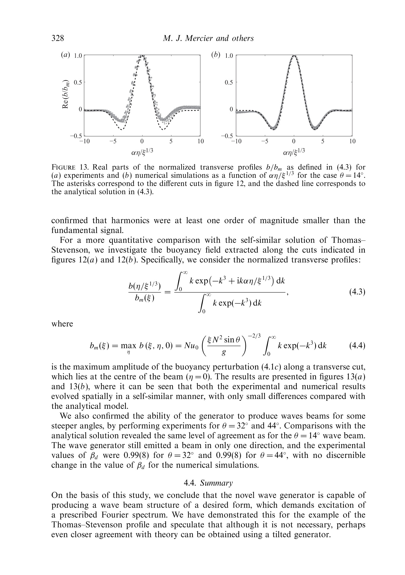
We present the results of a combined experimental and numerical study of the
generation of internal waves using the novel internal wave generator design of
Gostiaux et al. (Exp. Fluids, vol. 42, 2007, pp. 123–130). This mechanism, which
involves a tunable source composed of oscillating plates, has so far been used for a
few fundamental studies of internal waves, but its full potential is yet to be realized.
Our study reveals that this approach is capable of producing a wide variety of twodimensional
wave fields, including plane waves, wave beams and discrete vertical
modes in finite-depth stratifications. The effects of discretization by a finite number
of plates, forcing amplitude and angle of propagation are investigated, and it is found
that the method is remarkably efficient at generating a complete wave field despite
forcing only one velocity component in a controllable manner. We furthermore find
that the nature of the radiated wave field is well predicted using Fourier transforms
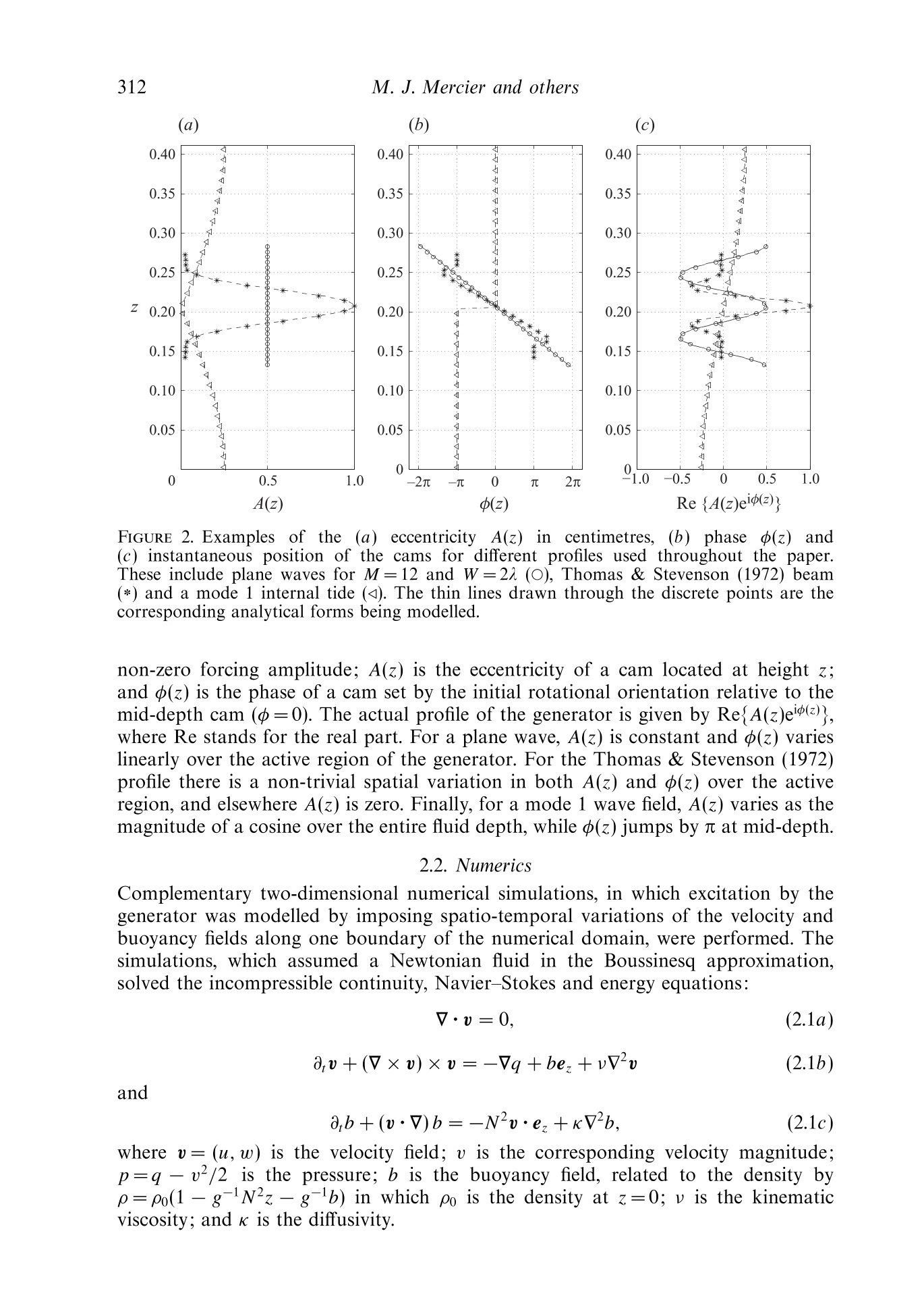
of the spatial structure of the wave generator.
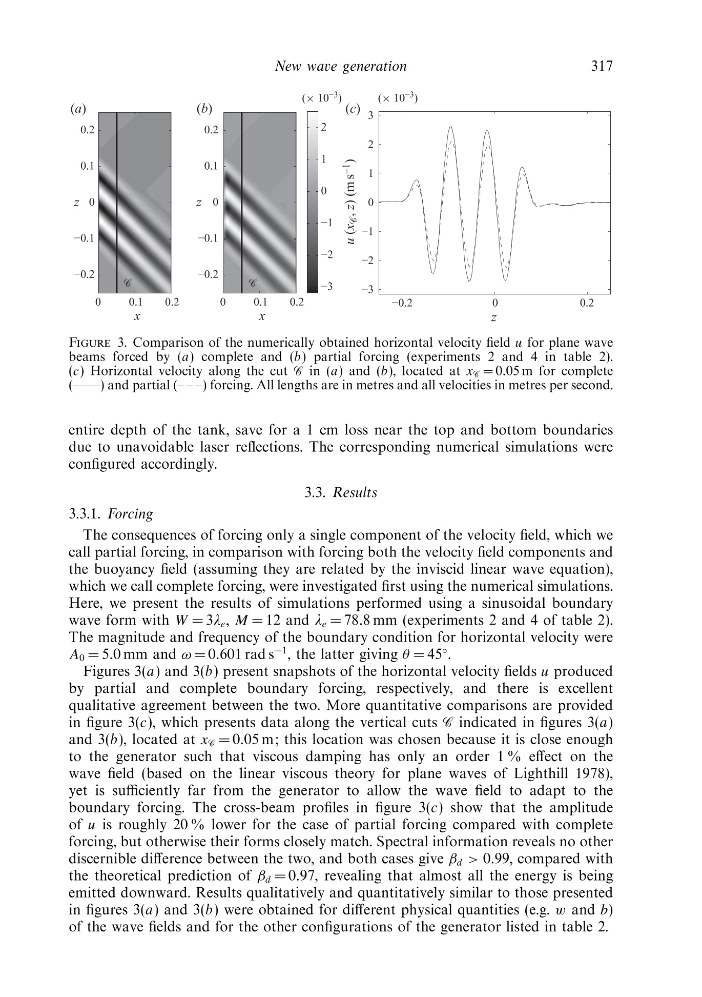
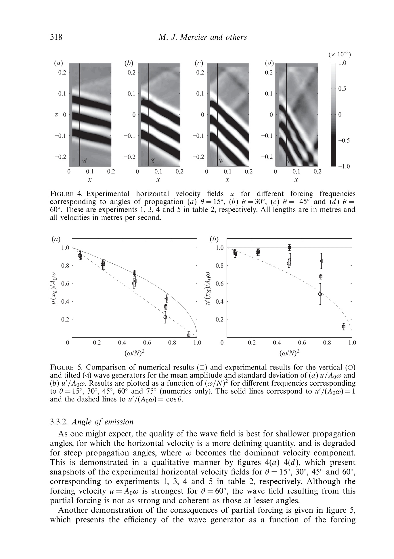
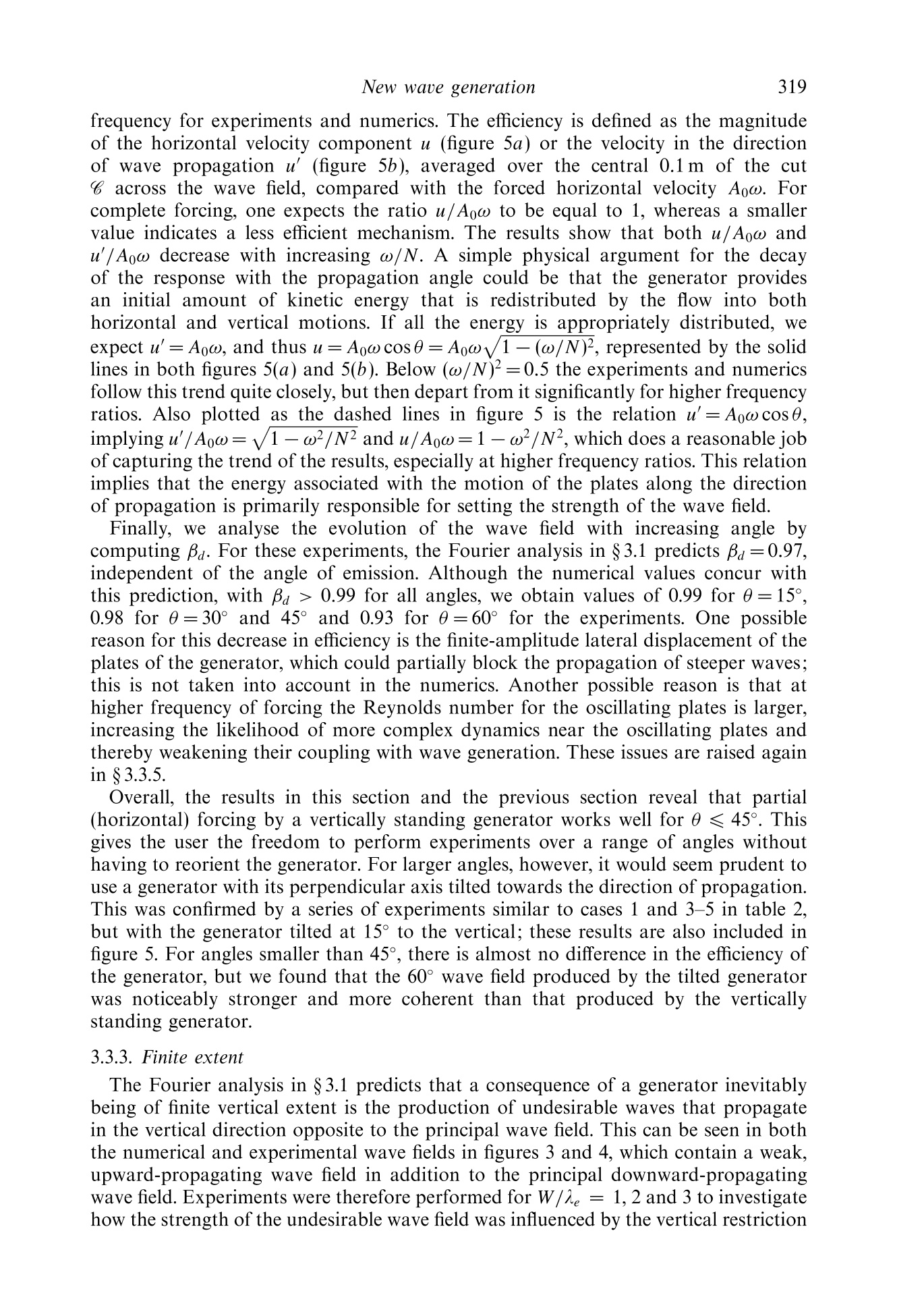
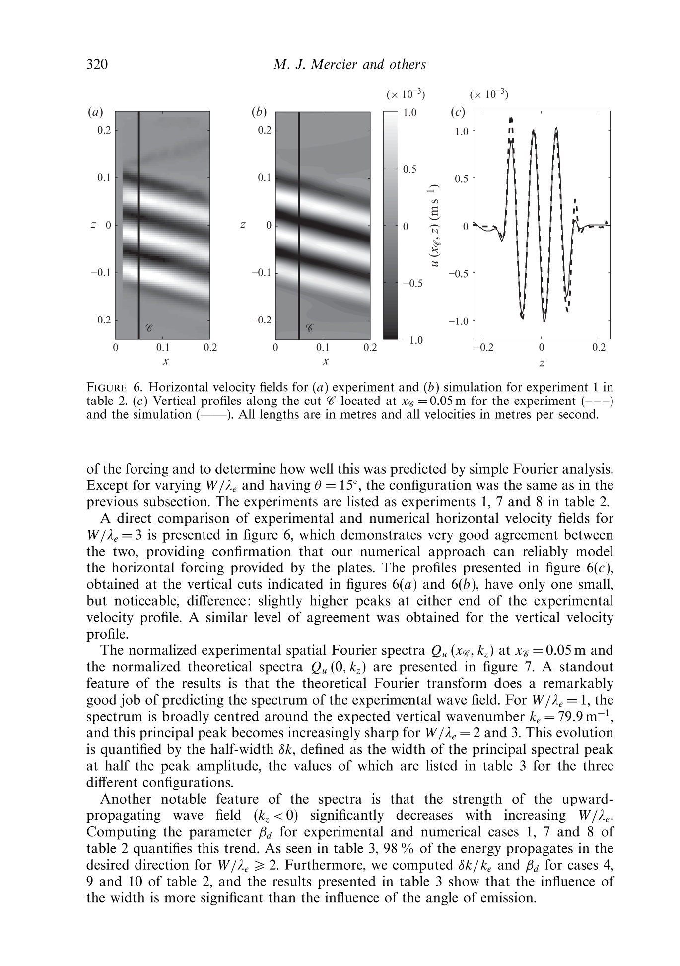
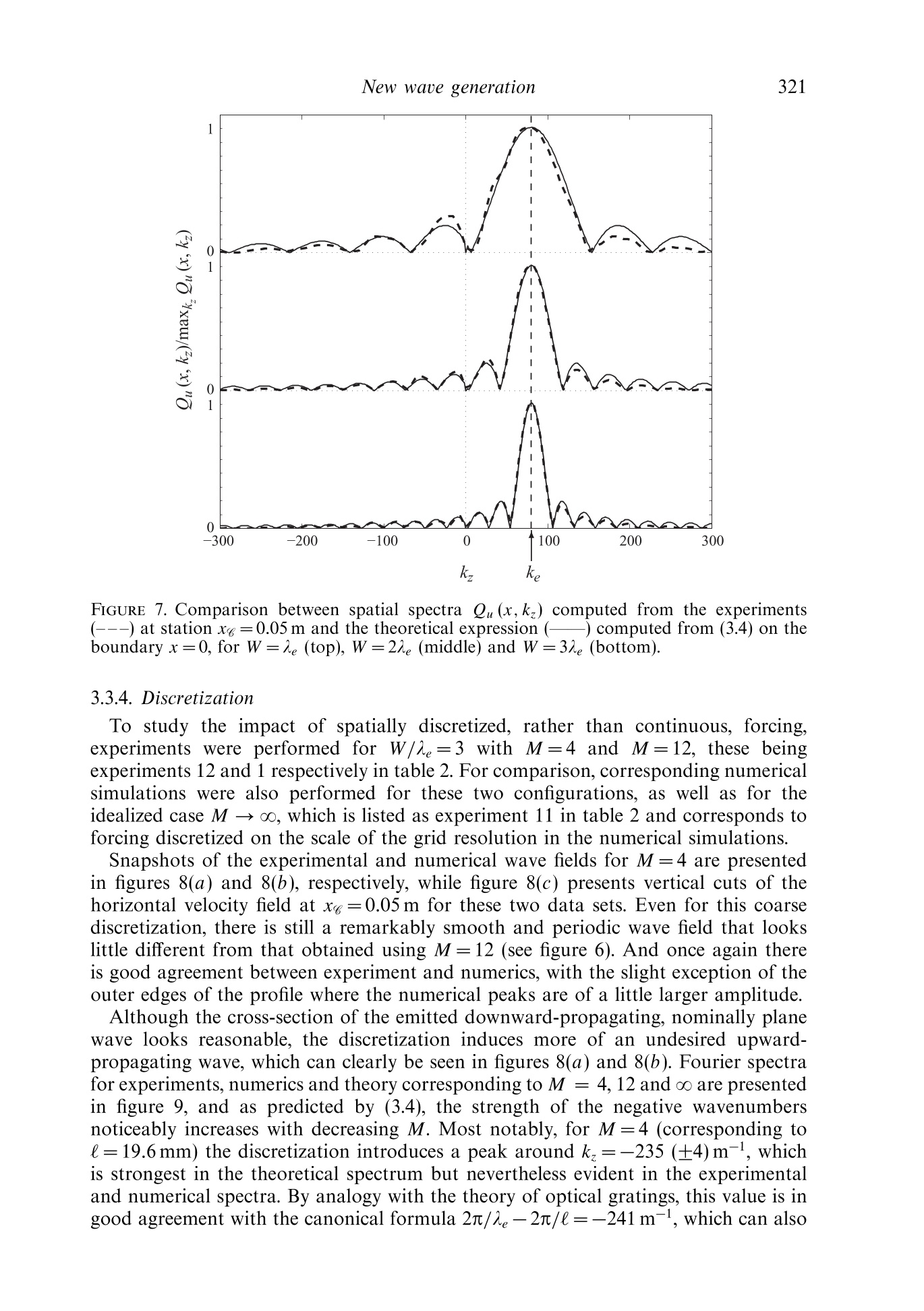
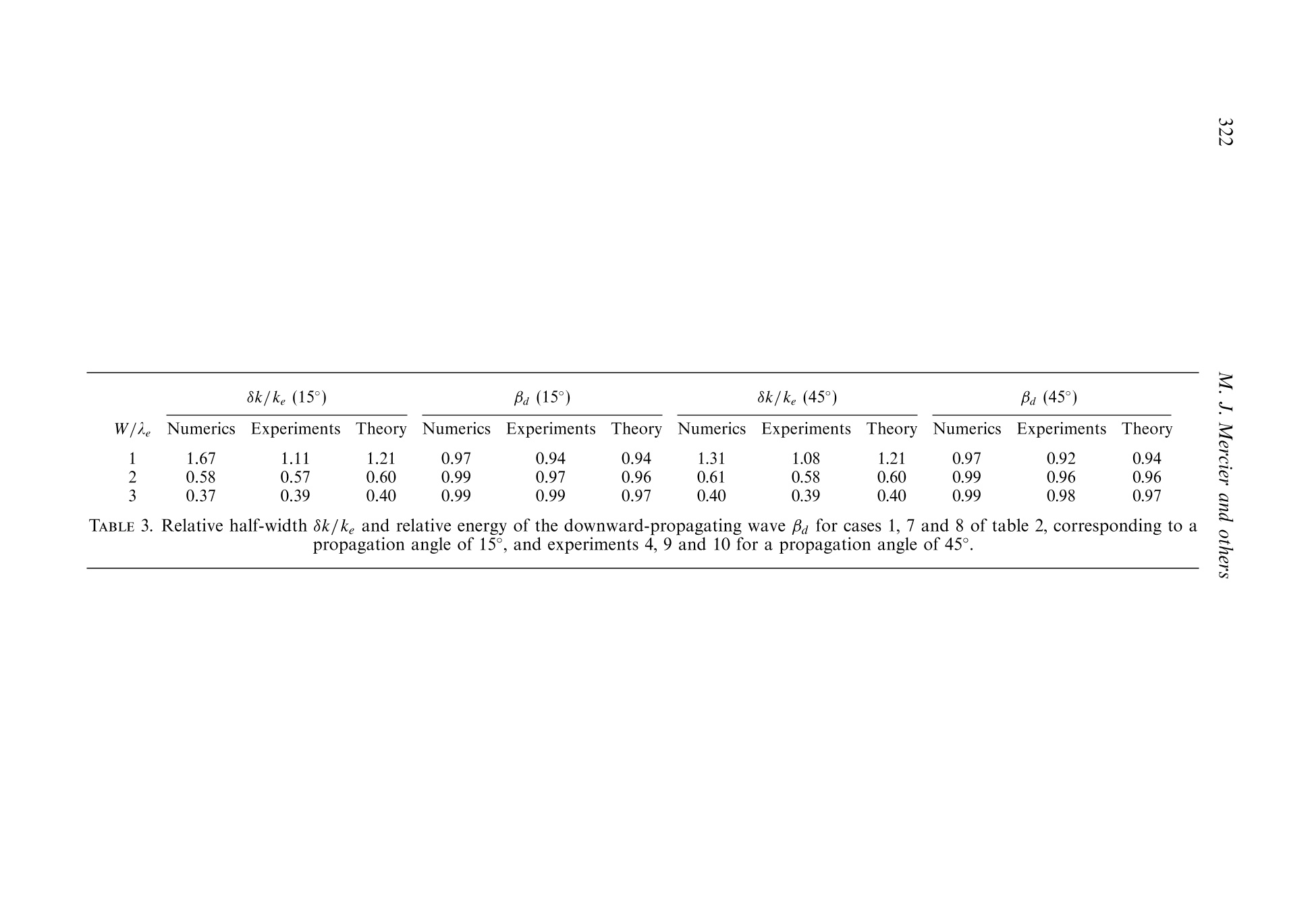
方案详情

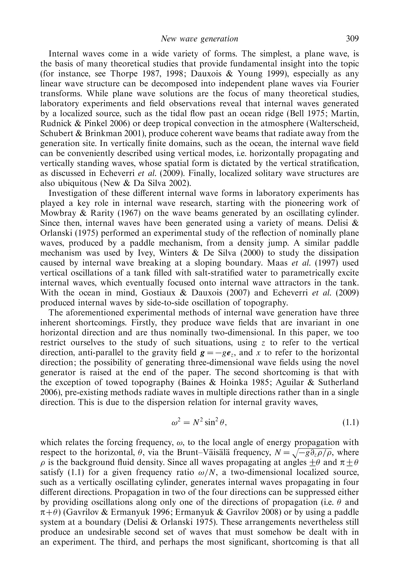
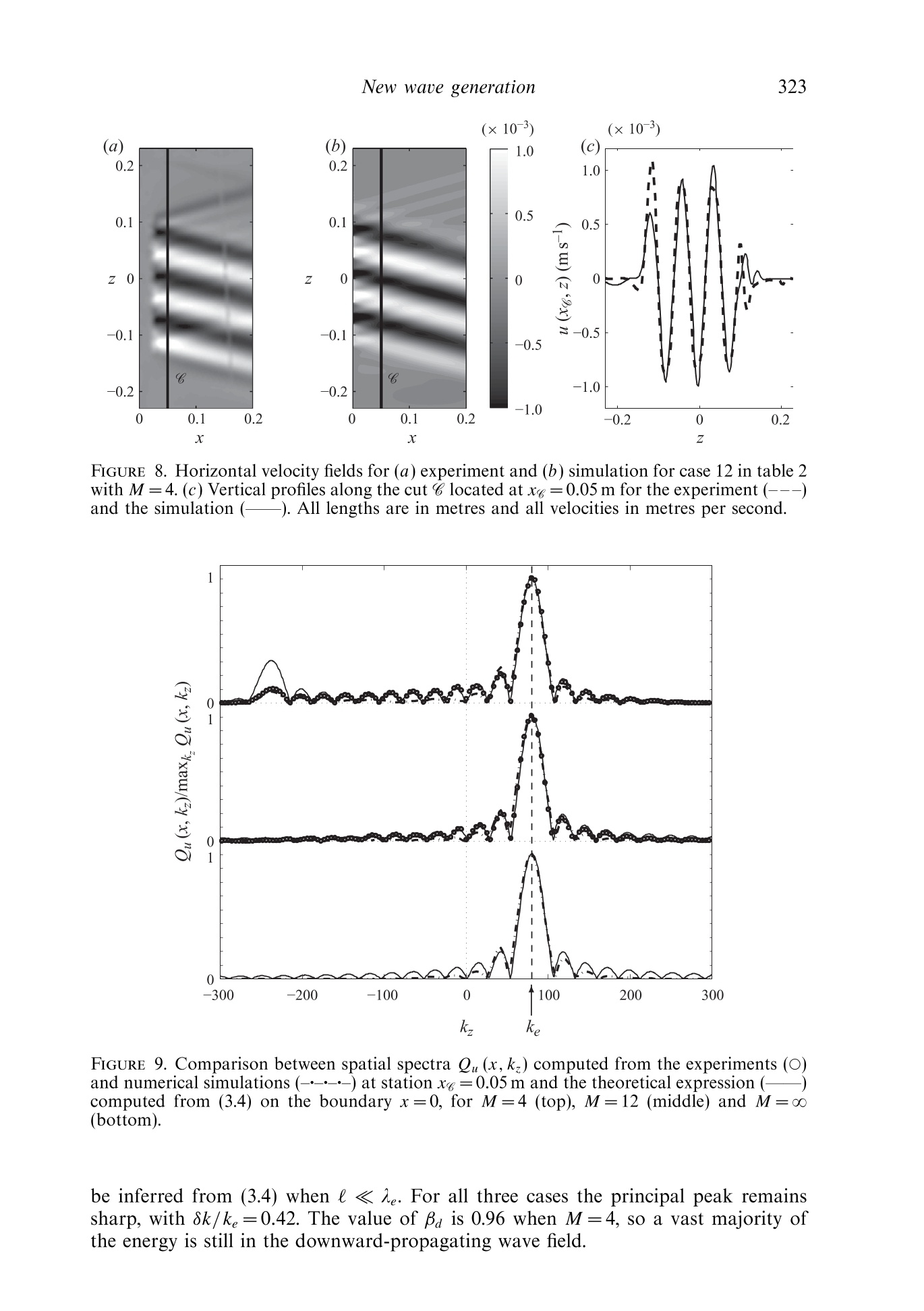
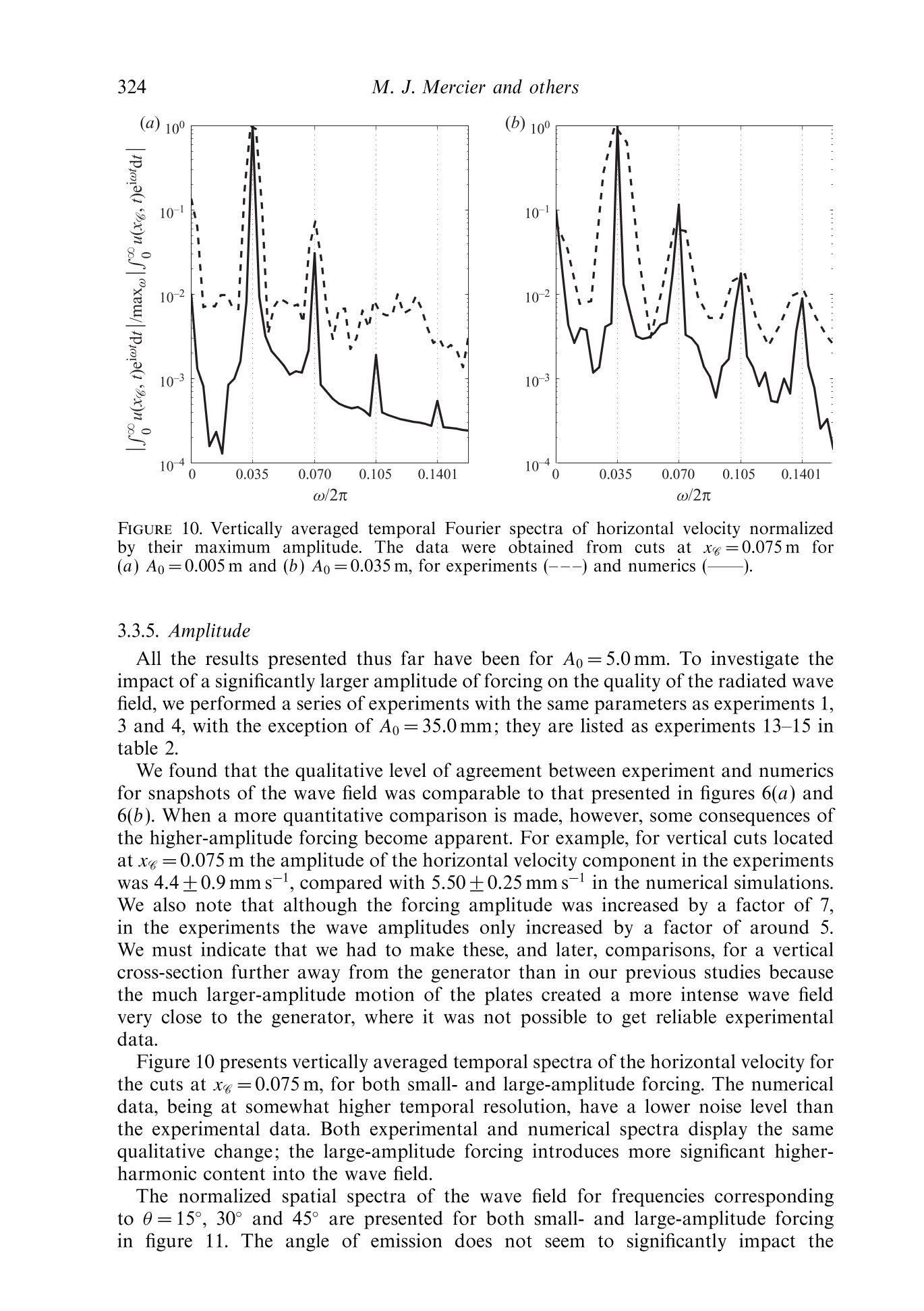
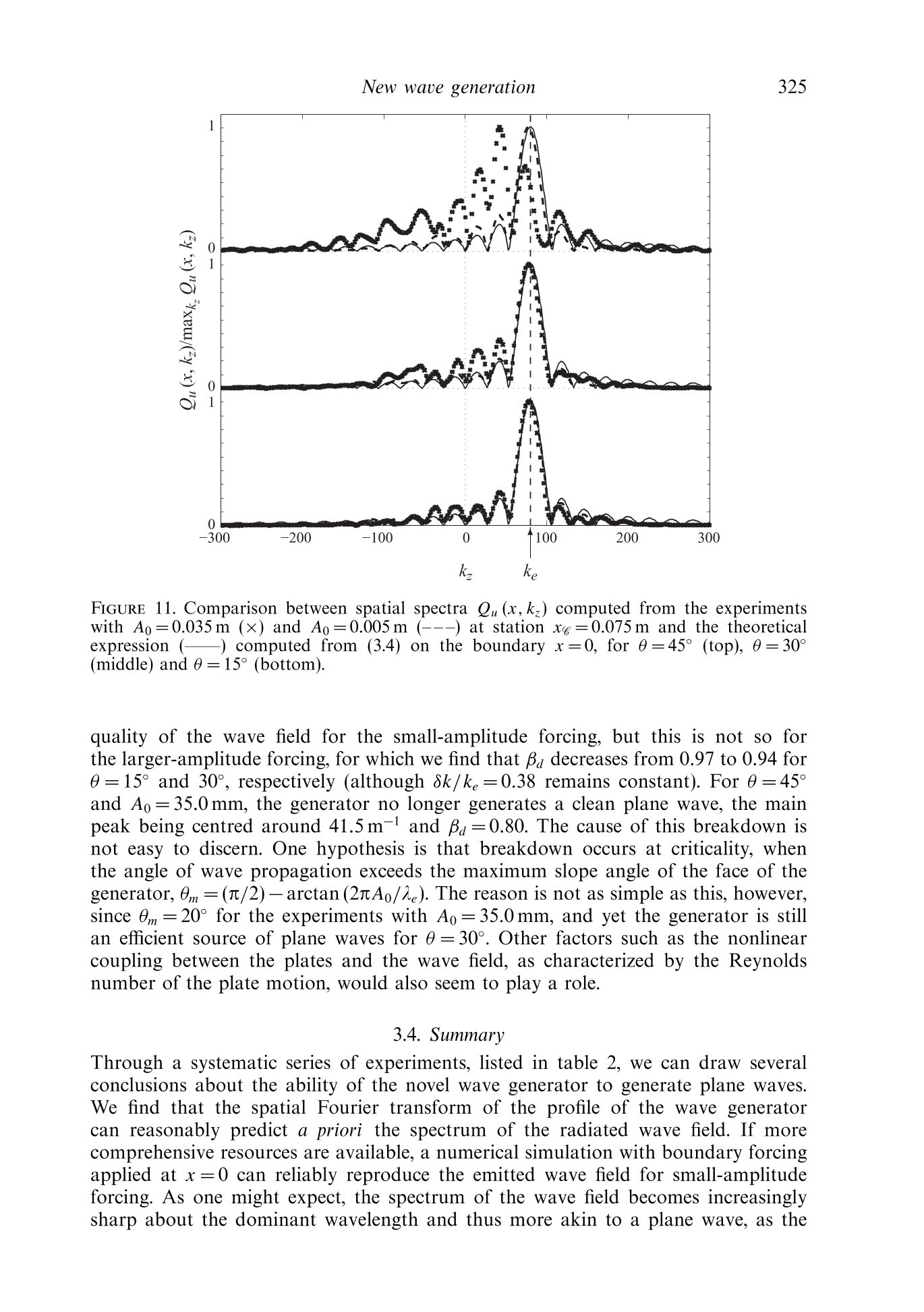
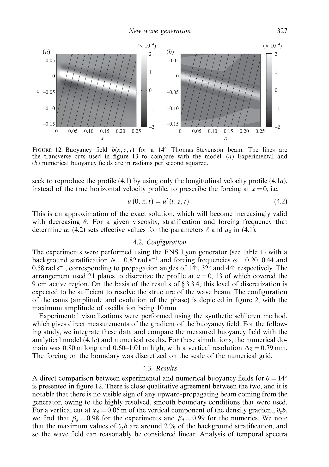
J. Fluid Mech. (2010), vol. 657, pp. 308-334.doi:10.1017/S0022112010002454C Cambridge University Press 2010 309New waue generation Email address for correspondence: matthieu.mercier@ens-lyon.fr New wave generation MATTHIEU J. MERCIER,DENIS MARTINAND,MANIKANDANMATHUR,LOUIS GOSTIAUX,THOMASPEACOCKAND THIERRY DAUXOIS Laboratoire de Physique de PEcole Normale Superieure de Lyon, CNRS-Universite de Lyon,Lyon 69364, France 2Laboratoire M2P2, UMR 6181 CNRS-Universites Aix-Marseille, Marseille 13451. France Department of Mechanical Engineering, Massachusetts Institute of Technology, Cambridge,MA 01239,USA 4Laboratoire des Ecoulements Geophysiques et Industriels (LEGI), CNRS, Grenoble 38000, France(Received 5 August 2009; revised 21 April 2010; accepted 21 April 2010) We present the results of a combined experimental and numerical study of thegeneration of internal waves using the novel internal wave generator design ofGostiaux et al. (Exp. Fluids, vol. 42, 2007, pp. 123-130). This mechanism, whichinvolves a tunable source composed of oscillating plates, has so far been used for afew fundamental studies of internal waves, but its full potential is yet to be realized.Our study reveals that this approach is capable of producing a wide variety of two-dimensional wave fields, including plane waves, wave beams and discrete verticalmodes in finite-depth stratifications.The effects of discretization by a finite numberof plates, forcing amplitude and angle of propagation are investigated, and it is foundthat the method is remarkably efficient at generating a complete wave field despiteforcing only one velocity component in a controllable manner. We furthermore findthat the nature of the radiated wave field is well predicted using Fourier transformsof the spatial structure of the wave generator. Key words: internal waves, stratified flows 1. Introduction The study of internal waves continues to generate great interest owing to theevolving appreciation of their role in many geophysical systems. In the ocean, internalwaves play an important role in dissipating barotropic tidal energy (see Garrett &Kunze 2007 for a review), whereas atmospheric internal waves are an important meansof momentum transport (Alexander, Richter & Sutherland 2006). In both the oceanand the atmosphere, internal wave activity also impacts modern-day technology(Osborne, Burch & Scarlet 1978). However, many unanswered questions remain,particularly regarding the fate of internal waves. For example, how much mixing dointernal waves generate in the ocean and via what processes? And at what altitudesdo atmospheric internal waves break and deposit their momentum? The ability toreliably model internal wave dynamics is key to tackling important questions such asthese. Internal waves come in a wide variety of forms. The simplest, a plane wave, isthe basis of many theoretical studies that provide fundamental insight into the topic(for instance, see Thorpe 1987, 1998; Dauxois & Young 1999), especially as anylinear wave structure can be decomposed into independent plane waves via Fouriertransforms. While plane wave solutions are the focus of many theoretical studies,laboratory experiments and field observations reveal that internal waves generatedby a localized source, such as the tidal flow past an ocean ridge (Bell 1975; Martin,Rudnick & Pinkel 2006) or deep tropical convection in the atmosphere (Walterscheid,Schubert & Brinkman 2001), produce coherent wave beams that radiate away from thegeneration site. In vertically finite domains, such as the ocean, the internal wave fieldcan be conveniently described using vertical modes, i.e. horizontally propagating andvertically standing waves, whose spatial form is dictated by the vertical stratification,as discussed in Echeverri et al. (2009). Finally, localized solitary wave structures arealso ubiquitous (New & Da Silva 2002). Investigation of these different internal wave forms in laboratory experiments hasplayed a key role in internal wave research, starting with the pioneering work ofMowbray & Rarity (1967) on the wave beams generated by an oscillating cylinder.Since then, internal waves have been generated using a variety of means. Delisi &Orlanski (1975) performed an experimental study of the reflection of nominally planewaves, produced by a paddle mechanism, from a density jump. A similar paddlemechanism was used by Ivey, Winters & De Silva (2000) to study the dissipationcaused by internal wave breaking at a sloping boundary. Maas et al. (1997) usedvertical oscillations of a tank filled with salt-stratified water to parametrically exciteinternal waves, which eventually focused onto internal wave attractors in the tank.With the ocean in mind, Gostiaux & Dauxois (2007) and Echeverri et al. (2009)produced internal waves by side-to-side oscillation of topography. The aforementioned experimental methods of internal wave generation have threeinherent shortcomings. Firstly, they produce wave fields that are invariant in onehorizontal direction and are thus nominally two-dimensional. In this paper, we toorestrict ourselves to the study of such situations, using z to refer to the verticaldirection, anti-parallel to the gravity field g=-ge, and x to refer to the horizontaldirection; the possibility of generating three-dimensional wave fields using the novelgenerator is raised at the end of the paper. The second shortcoming is that withthe exception of towed topography (Baines & Hoinka 1985; Aguilar & Sutherland2006), pre-existing methods radiate waves in multiple directions rather than in a singledirection. This is due to the dispersion relation for internal gravity waves, which relates the forcing frequency, ω, to the local angle of energy propagation withrespect to the horizontal, 0, via the Brunt-Vaisaila frequency, N=-go p/p, wherep is the background fluid density. Since all waves propagating at angles ±0 and n±0satisfy (1.1) for a given frequency ratio w/N, a two-dimensional localized source,such as a vertically oscillating cylinder, generates internal waves propagating in fourdifferent directions. Propagation in two of the four directions can be suppressed eitherby providing oscillations along only one of the directions of propagation (i.e. 0andn+0) (Gavrilov & Ermanyuk 1996; Ermanyuk & Gavrilov 2008) or by using a paddlesystem at a boundary (Delisi & Orlanski 1975). These arrangements nevertheless stillproduce an undesirable second set of waves that must somehow be dealt with inan experiment. The third, and perhaps the most significant, shortcoming is that all FIGURE 1. A schematic showing the basic configuration of a novel internal wave generator.The plates are vertically stacked on an eccentric camshaft. See 82 for the definitions of thedifferent lengths W, l and 1. The circular arrow at the top of the generator illustrates thedirection of rotation of the camshaft; the thick vertical arrows show the corresponding motionof the wave form of the plates; and the dashed oblique arrows indicate the resulting localvelocity field. Further, uo and u indicate the direction of the phase and group velocities,respectively. pre-existing methods provide very limited, if any, control of the spatial structure ofan internal wave field. A major advance in internal wave generation recently occurred with the design of anovel type of internal wave generator (Gostiaux et al. 2007). This design uses a seriesof stacked, offset plates on a camshaft to simultaneously shape the spatial structure ofan experimental internal wave field and enforce wave propagation in a single direction,as illustrated in figure 1. The maximum horizontal displacement of each plate is setby the eccentricity of the corresponding cam, and the spatio-temporal evolution isdefined by the phase progression from one cam to another and the rotation speed ofthe camshaft. So far, this configuration has been used to study plane wave reflectionfrom sloping boundaries (Gostiaux 2006), diffraction through a slit (Mercier, Garnier& Dauxois 2008) and wave beam propagation through non-uniform stratifications(Mathur & Peacock 2009). Despite these early successes, however, there has been nodedicated study of the ability of this arrangement to generate qualitatively differentforms of internal wave fields, and several important questions remain. For example,how does a stratified fluid that supports two-dimensional waves respond to controlledforcing in only one direction (i.e. parallel to the motion of the plates)? In this paper, we present the results of a comprehensive study of two-dimensionalwave fields produced by different configurations of novel internal wave generators andreveal that this approach can accurately produce plane waves, wave beams and discretevertical modes. The results of experiments are compared with predictions based onthe Fourier transforms of the spatial structure of the wave generator, which proves tobe a very useful and simple tool for predicting wave fields, and numerical simulations,which allow investigation of the boundary conditions imposed by the generator.The paper is organized as follows: 82 presents the experimental and nummethods used throughout the study. The generation of plane waves is addressed inS3, followed by the generation of self-similar wave beams and vertical modes in $s4and 5, respectively. Our conclusions, and suggestions for future applications of thegenerator, are presented in $6. Generator Height Width Plate thickness Plate gap Maximum eccentricity Number of plates ENS 390.0 140.0 6.0 0.7 10.0 60 MIT 534.0 300.0 6.3 0.225 35.0 82 TABLE 1. Details of the wave generators at ENS de Lyon and Massachusetts Institute ofTechnology (MIT). Dimensions are in millimetres. 2. Methods 2.1. Experiments Throughout this paper, we consider the case of wave fields excited by a verticallystanding generator with horizontally moving plates of thickness l, as depicted infigure 1. This scenario, which is possible because the direction of wave propagationis set by the dispersion relation (1.1), has two major advantages over the otherpossibility of a generator tilted in the direction of wave propagation (Gostiaux et al.2007; Mathur & Peacock 2009). First, it is far more convenient because it requiresno mechanical components to orient the camshaft axis and no change of orientationfor different propagation angles. Second, unwanted wave beams that are inevitablyproduced by free corners within the body of a stratified fluid are eliminated becausethe generator extends over the entire working height of the fluid. Two different laboratory experimental facilities, both using the double-bucketmethod (Oster 1965) to create salt/density stratifications, were used. The first, atEcole Normale Superieure (ENS) de Lyon, utilized a 0.8 m long, 0.170m wide and0.425 m deep wave tank. The wave generator, whose characteristics are listed in table 1,was positioned at one end of the tank. On each side of the wave generator therewas a 0.015m gap between the moving plates and the side wall of the wave tank.Visualizations and quantitative measurements of the density-gradient perturbationfield were performed using the synthetic schlieren technique (Dalziel, Hughes &Sutherland 2000). The correlation imaging velocimetry algorithm of Fincham &Delerce (2000) was used to compute the cross-correlation between the real-timeand the t=0 background images. Blocksom filter matting was used to effectivelydamp end-wall reflections of internal waves. The ENS Lyon set-up was used to runexperimental studies of the classical Thomas-Stevenson wave beam profile (Thomas& Stevenson 1972), detailed in $ 4. The second system, at MIT, utilized a 5.5m long, 0.5m wide and 0.6m deepwave tank. A partition divided almost the entire length of the tank into 0.35 and0.15 m wide sections, the experiments being performed in the wider section. The wavegenerator, whose characteristics are given in table 1, was mounted in the 0.35 m widesection of the tank with a gap of 0.025m between the moving plates and eitherside wall. Parabolic end walls at the ends of the wave tank reflected the wave fieldproduced by the generator into the 0.15 m wide section of the tank, where it wasdissipated by Blocksom filter matting. Visualizations and quantitative measurementsof the velocity field in the vertical midplane of the generator were obtained using aLaVision particle image velocimetry(PIV) system. This facility was used for studiesof plane waves and vertical modes,detailed in $$3 and 5, respectively. Examples of the amplitude and phase arrangements of the plates for the experimentsdiscussed in this paper are presented in figure 2. We use the following terminology:M is the number of plates per period, used to represent a periodic wave form ofvertical wavelength A; W is the total height of the active region of the generator with FIGURE 2. Examples of the (a) eccentricity A(z) in centimetres,(b) phase 人(z)and(c) instantaneous position of the cams for different profiles used throughout the paper.These include plane waves for M=12 and W=21(O), Thomas & Stevenson (1972) beam(*) and a mode 1 internal tide (<). The thin lines drawn through the discrete points are thecorresponding analytical forms being modelled. non-zero forcing amplitude; A(z) is the eccentricity of a cam located at height z;and d(z) is the phase of a cam set by the initial rotational orientation relative to themid-depth cam (中=0). The actual profile of the generator is given by Re{A(z)eld(2)},where Re stands for the real part. For a plane wave, A(z) is constant and d(z) varieslinearly over the active region of the generator. For the Thomas & Stevenson (1972)profile there is a non-trivial spatial variation in both A(z) and (z) over the activeregion, and elsewhere A(z) is zero. Finally, for a mode 1 wave field, A(z) varies as themagnitude of a cosine over the entire fluid depth, while (z) jumps by n at mid-depth. 2.2. Numerics Complementary two-dimensional numerical simulations, in which excitation by thegenerator was modelled by imposing spatio-temporal variations of the velocity andbuoyancy fields along one boundary of the numerical domain, were performed. Thesimulations, which assumed a Newtonian fluid in the Boussinesq approximation,solved the incompressible continuity, Navier-Stokes and energy equations: and where u=(u, w) is the velocity field; u is the corresponding velocity magnitude;p=q-u2/2 is the pressure; b is the buoyancy field, related to the density byp=po(1-g-N’z-g-lb) in which po is the density at z=0; v is the kinematicviscosity; and k is the diffusivity. The code used was an extension of that developed for channel flow (Gilbert 1988),to which the integration of the energy equation and the possibility of spatially varyingand time-evolving boundary conditions on the plates were added, as already presentedin Martinand, Carriere & Monkewitz (2006) for thermal convection. The methodproceeds as follows. A numerical solution in a rectangular domain [0,1.]×[0,1,]is obtained by a tau-collocation pseudo-spectral method in space, using Fouriermodes in the z-direction and Chebyshev polynomials in the confined x-direction. Thismethod very precisely accounts for the dissipative terms. The nonlinear and diffusionterms are discretized in time by Adams-Bashforth and Crank-Nicolson schemes,respectively, resulting in second-order accuracy in time. As the simulation focuseson the linear and weakly nonlinear dynamics, the de-aliasing of the nonlinear termin the spatial expansion of the solution is not of crucial importance and is omittedto decrease the computational cost. Owing to the assumption of a divergence-freeflow, the influence matrix method, introduced in Kleiser & Schumann (1980, 1984),is used to evaluate the pressure and the velocity field, the pressure gradient in theNavier-Stokes equation then being discretized by an implicit Euler scheme. Finally,the buoyancy term is also discretized in time by an implicit Euler scheme, since theenergy equation is solved before the Navier-Stokes equations. Simulations were run by imposing forced boundary conditions on components ofthe velocity and buoyancy fields at x=0; no forcing was applied to the pressure, sinceits value on the boundaries is an outcome of the numerical method. The governingequations (2.1) were thus integrated together with Dirichlet boundary conditions, while were applied at x=l.. We note that this numerical forcing is Eulerian in nature,whereas the corresponding experimental forcing is Lagrangian in spirit. The spectralmethod introduces periodic conditions in the z-direction, which have to be accountedfor to avoid Gibbs oscillations. Therefore, the boundary conditions (2.2)Weremultiplied by a polynomial “hat'function H(z)=(1-(2z/lz-1)30)6, vanishing atz=0 and z=1.The choice of the exponents in H(z) is qualitative, the aim being thatthe variation of the profile envelope is smooth compared with the spatial resolution,yet sharp enough to keep a well-defined width of forcing. The boundary conditions (2.3) imply wave reflection, with the reflected waveseventually interfering with the forced waves. Thus, the numerical domain was madesufficiently large to establish the time-periodic forced wave field near the generationlocation long before reflections became an issue. For a typical simulation, the domainwas lx=3.01 m long and l=1.505m high, and the number of grid points used wasNx=1024 and N =512, giving a spatial vertical resolution of 2.9 mm that ensured atleast two grid points per plate. Satisfactory spectral convergence was confirmed forthis spatial resolution, and the time step was set to ensure stability of the numericalscheme. 2.3. Analysis A detailed study of the impact of sidewall boundary conditions on the generationof shear waves was performed by McEwan & Baines (1974). Here, we take asimpler approach and show that a useful tool for investigating both theoreticaland experimental internal wave fields produced by the novel generator is Fourier analysis. This allows one to decompose internal wave fields into constituent planewaves and readily make predictions about the radiated wave field. For an unconfined inviscid two-dimensional system, any physical field variableassociated with a periodic internal wave field of frequency ω can be described by itsFourier spectrum (Tabaei & Akylas 2003; Tabaei,Akylas & Lamb 2005), i.e. where y(x,z, t) represents a field variable (e.g. b, u) and the Dirac 8-function ensuresthe dispersion relation (1.1) is satisfied by the plane wave components. Propagatingwaves in a single direction, say towards the positive x-component and the negativez-component for the energy propagation, require as noted by Mercier et al. (2008). At a fixed horizontal location xo, the values of y(xo,z, t) for all the field variablescan be considered as boundary conditions that force the propagating wave fieldw(x,z,t). Knowing the Fourier transform of the boundary forcing, leads to the complete description of the radiated wave field for x > xo. assuming that only right-propagating waves (i.e.kx≥0) are possible. In practice, the novel wave generator we consider forces only the horizontal velocityfield in a controlled manner, i.e. As such, we expect the Fourier transform of this boundary condition to act only asa guide for the nature of the radiated wave field, since it is not clear how the fluidwill respond to forcing of a single field variable. Throughout the paper, we performthe Fourier transform along a specific direction using the fast Fourier transformalgorithm. To compare spectra from theoretical, numerical and experimental profileswith the same resolution, a cubic interpolation (in space) of the experimental wavefield is used if needed. Unless otherwise stated, the experimental and numerical results presentedarefiltered in time at the forcing frequency w. The aim is to consider harmonic (intime) internal waves for which we can define the Fourier decomposition in (2.4) andto improve the signal-to-noise ratio, which lies in the range 102-10, with the bestresults for shallow beam angles and small-amplitude forcing. The time window Atused for the filtering is such that ω▲t/2n ≥ 9 for Ao=0.005m and w▲t/2元 ≥ 4 forAo=0.035m (where Ao is the amplitude of motion of the plates defined in (3.1)),ensuring sufficient resolution in Fourier space for selective filtering. The recordingwas initiated at time to after the start-up of the generator such that Nto/2n30>1,ensuring no transients remained (Voisin 2003). Experiment Experiment/simulation Forcing M W/1e Ao (mm) 0 (deg.) Common case 1 Experiment/simulation Partial 12 3 5.0 15 Forcing 2 Simulation Complete 12 3 5.0 45 3 Experiment/simulation Partial 12 3 5.0 30 Angle 4 Experiment/simulation Partial 12 3 5.0 45 5 Experiment/simulation Partial 12 3 5.0 60 6 Simulation Partial 12 3 5.0 75 7 Experiment/simulation Partial 12 2 5.0 15 Width 8 Experiment/simulation Partial 12 1 5.0 15 9 Experiment/simulation Partial 12 2 5.0 45 10 Experiment/simulation Partial 12 1 5.0 45 Discretization 11 Simulation Partial 00 3 5.0 15 12 Experiment/simulation Partial 4 3 5.0 15 Amplitude 13 Experiment/simulation Partial 12 3 35.0 15 14 Experiment Partial 12 3 35.0 30 15 Experiment Partial 12 3 35.0 45 TABLE 2. Summary of experiments and numerical simulations: M is the number of plates usedfor one wavelength; W/a is the spatial extent of forcing expressed in terms of the dominantwavelength; Ao is the eccentricity of the cams; and 0 is the energy propagation angle. Forcomplete forcing,u, w and b were forced at the boundary. 3. Plane waves Since many theoretical results for internal waves are obtained for plane waves(e.g. Thorpe 1987, 1998;Dauxois & Young 1999), the ability to generate a goodapproximation of a plane wave in a laboratory setting is important to enablecorresponding experimental investigations. In order to generate a nominally planewave, however, one must consider the impact of the different physical constraintsof the wave generator, which include the controlled forcing of only one velocitycomponent by the moving plates, the finite spatial extent of forcing, the discretizationof forcing by a finite number of plates, the amplitude of forcing and the direction ofwave propagation with respect to the camshaft axis of the generator. In this section,we present the results of a systematic study of the consequences of these constraints;a summary of the experiments is presented in table 2. 3.1. Analysis Two-dimensional, planar internal waves take the form v(x,z, t)=Re{yoe(ikrx+ikz-iot)),where k=(k,kz) is the wave vector and w(x,z,t) represents a field variable. Beingof infinite extent is an idealization that is never realizable in an experiment. Toinvestigate the consequences of an internal wave generator being of finite extent,the horizontal velocity boundary conditions used to produce a downward right-propagating nominally plane wave can be written as where ke>0 is the desired vertical wavenumber, 1e=2n/k, the corresponding verticalwavelength, -W/2≤z ≤ W/2 the vertical domain over which forcing is applied,Ao the amplitude of motion of the plates and the Heaviside function. The spatial Fourier transform of (3.1) is with sinc(x)= sin x/x the sine cardinal function. In the limit W→0,(3.2) approachesa 8-function, which is the Fourier transform of a plane wave. Owing to the finite valueof W, however, Qu(0,kz) does not vanish for negative values of kz, suggesting that(3.1) will also excite upward-propagating plane waves. Following the convention usualin optics that Qu(0,k) is negligible for |kz-ke|W/2≥, if ke> 2元/W, then (2.5) isreasonably satisfied. Another consideration is that the forcing provided by the wave generator is notspatially continuous but discretized by N, oscillating plates of width l. Accountingfor this, the boundary forcing can be written as where zj=jl-W/2 and N,l=W. The Fourier transform of (3.3) for the specificcase of constant amplitudes, A(zj)= Aoω, Vje{0,...,N,-1}, reduces to aclassical result often encountered for diffraction gratings. Consequently, themagnitudes of W and l in comparison with the desired vertical wavelength Ae=2n/k,characterize the spread of the Fourier spectrum and the potential for excitation ofupward-propagating waves. In the following sections, we quantify the downward emission of waves using theparameter Ba, defined as 00 which is essentially the ratio of the total kinetic energy of the downward-propagatingwaves to the total kinetic energy of the radiated wave field. 3.2. Configuration The MIT facility was used for these plane wave experiments (see table 1). A varietyof different configurations were tested, which are summarized in table 2. The fluiddepth was H=0.56±0.015 m, and the background stratification was N =0.85 rad s-for all experiments. An example configuration of the cams (amplitude and re?phaseevolution) is presented in figure 2. Plane waves were produced by configuring N,plates of the wave generator with an oscillation amplitude Ao=0.005m, with theexception of experiments 13-15 for which Ao=0.035 m. Results were obtained fordifferent forcing frequencies corresponding to propagating angles of 15°, 30°, 45°and 60°. Visualization of the wave field was performed using PIV, for which itwas possible to observe the wave field in a 40 cm wide horizontal domain over the FIGURE 3. Comparison of the numerically obtained horizontal velocity field u for plane wavebeams forced by (a) complete and (b) partial forcing (experiments 2 and 4 in table 2).(c) Horizontal velocity along the cut B in (a) and (b), located at xg=0.05 m for complete(—) and partial (---) forcing. All lengths are in metres and all velocities in metres per second. entire depth of the tank, save for a 1 cm loss near the top and bottom boundariesdue to unavoidable laser reflections. The corresponding numerical simulations wereconfigured accordingly. 3.3. Results 3.3.1. Forcing The consequences of forcing only a single component of the velocity field, which wecall partial forcing, in comparison with forcing both the velocity field components andthe buoyancy field (assuming they are related by the inviscid linear wave equation),which we call complete forcing, were investigated first using the numerical simulations.Here, we present the results of simulations performed using a sinusoidal boundarywave form with W=31e, M=12 and 1e=78.8 mm (experiments 2 and 4 of table 2).The magnitude and frequency of the boundary condition for horizontal velocity wereAo=5.0 mm and ω=0.601 rads, the latter giving 0=45°. Figures 3(a) and 3(b) present snapshots of the horizontal velocity fields u producedby partial and complete boundary forcing, respectively, and there is excellentqualitative agreement between the two. More quantitative comparisons are providedin figure 3(c), which presents data along the vertical cuts 《indicated in figures 3(a)and 3(b), located at xg=0.05 m; this location was chosen because it is close enoughto the generator such that viscous damping has only an order 1% effect on thewave field (based on the linear viscous theory for plane waves of Lighthill 1978),yet is sufficiently far from the generator to allow the wave field to adapt to theboundary forcing. The cross-beam profiles in figure 3(c) show that the amplitudeof u is roughly 20% lower for the case of partial forcing compared with completeforcing, but otherwise their forms closely match. Spectral information reveals no otherdiscernible difference between the two, and both cases give βa >0.99,compared withthe theoretical prediction of βa=0.97, revealing that almost all the energy is beingemitted downward. Results qualitatively and quantitatively similar to those presentedin figures 3(a) and 3(b) were obtained for different physical quantities (e.g. w and b)of the wave fields and for the other configurations of the generator listed in table 2. FIGURE 4. Experimentalhorizontal.velocity fields for different forcing frequencie:corresponding to angles of propagation (a) 0=15°, (b)0=30°, (c) 0=45°and(d) 0=60°. These are experiments 1, 3, 4 and 5 in table 2, respectively. All lengths are in metres andall velocities in metres per second. FIGURE 5. Comparison of numerical results (口) and experimental results for the vertical (O)and tilted (<) wave generators for the mean amplitude and standard deviation of (a) u/Aoω and(b)u’/Aoω. Results are plotted as a function of (ω/N)2 for different frequencies correspondingto 0=15, 30°,45°, 60° and 75° (numerics only). The solid lines correspond to u'/(Aoω)=1and the dashed lines to u'/(Aoω)= cos 0. 3.3.2. Angle of emission As one might expect, the quality of the wave field is best for shallower propagationangles, for which the horizontal velocity is a more defining quantity, and is degradedfor steep propagation angles, where w becomes the dominant velocity component.This is demonstrated in a qualitative manner by figures 4(a)-4(d), which presentsnapshots of the experimental horizontal velocity fields for 0=15°, 30°, 45° and 60°,corresponding to experiments 1, 3, 4 and 5 in table 2, respectively. Although theforcing velocity u=Aoω is strongest for 0=60°, the wave field resulting from thispartial forcing is not as strong and coherent as those at lesser angles. Another demonstration of the consequences of partial forcing is given in figure 5,which presents the efficiency of the wave generator as a function of the forcing frequency for experiments and numerics. The efficiency is defined as the magnitudeof the horizontal velocity component u (figure 5a) or the velocity in the directionof wave propagation u' (figure 5b), averaged over the central 0.1m of the cutacross the wave field, compared with the forced horizontal velocity Aoω. Forcomplete forcing, one expects the ratiou/Agω to be equal to 1, whereas a smallervalue indicates a less efficient mechanism. The results show that both u/Aoω andu'/Aoω decrease with increasing ω/N. A simple physical argument for the decayof the response with the propagation angle could be that the generator providesan initial amount of kinetic energy that is redistributed by the flow into bothhorizontal and vertical motions. If all the energy is appropriately distributed, weexpect u'= Aoω, and thus u=Aoω cos0=Agω√1-(ω/N)2, represented by the solidlines in both figures 5(a) and 5(b). Below (ω/N)2=0.5 the experiments and numericsfollow this trend quite closely, but then depart from it significantly for higher frequencyratios. Also plotted as the dashed lines in figure 5 is the relation u'=Aoω cos 0,implying u'/Aoω=√1-w²/N2andu/Aoω=1-ω/N2, which does a reasonable jobof capturing the trend of the results, especially at higher frequency ratios. This relationimplies that the energy associated with the motion of the plates along the directionof propagation is primarily responsible for setting the strength of the wave field. Finally, we analyse the evolution of the wave field with increasing angle bycomputing Ba. For these experiments, the Fourier analysis in $3.1 predicts Ba=0.97,Hin山deeFpendent of the angle of emission. Although the numerical values concur withthis prediction, with βa > 0.99 for all angles, we obtain values of 0.99 for 0=15°0.98 for 0=30° and 45°and 0.93 for 0=60°for the experiments. One possiblereason for this decrease in efficiency is the finite-amplitude lateral displacement of theplates of the generator, which could partially block the propagation of steeper waves;this is not taken into account in the numerics. Another possible reason is that athigher frequency of forcing the Reynolds number for the oscillating plates is larger,increasing the likelihood of more complex dynamics near the oscillating plates andthereby weakening their coupling with wave generation. These issues are raised againin s3.3.5. .Overall, the results in this section and the previous section reveal that partial(horizontal) forcing by a vertically standing generator works well for 0 ≤ 45°. Thisgives the user the freedom to perform experiments over a range of angles withouthaving to reorient the generator. For larger angles, however, it would seem prudent touse a generator with its perpendicular axis tilted towards the direction of propagation.This was confirmed by a series of experiments similar to cases 1 and 3-5 in table 2,but with the generator tilted at 15°to the vertical; these results are also included infigure 5. For angles smaller than 45°, there is almost no difference in the efficiency ofthe generator, but we found that the 60°wave field produced by the tilted generatorwas noticeably stronger and more coherent than that produced by the verticallystanding generator. 3.3.3. Finite extent The Fourier analysis in $3.1 predicts that a consequence of a generator inevitablybeing of finite vertical extent is the production of undesirable waves that propagatein the vertical direction opposite to the principal wave field. This can be seen in boththe numerical and experimental wave fields in figures 3 and 4, which contain a weak,upward-propagating wave field in addition to the principal downward-propagatingwave field. Experiments were therefore performed for W/ae = 1, 2 and 3 to investigatehow the strength of the undesirable wave field was influenced by the vertical restriction FIGURE 6. Horizontal velocity fields for (a) experiment and (b) simulation for experiment 1 intable 2. (c) Vertical profiles along the cut 《located at xg=0.05 m for the experiment (---)and the simulation (——). All lengths are in metres and all velocities in metres per second. of the forcing and to determine how well this was predicted by simple Fourier analysis.Except for varying W/ae and having0=15°, the configuration was the same as in theprevious subsection. The experiments are listed as experiments 1, 7 and 8 in table 2. A direct comparison of experimental and numerical horizontal velocity fields forW/1e=3is presented in figure 6, which demonstrates very good agreement betweenthe two, providing confirmation that our numerical approach can reliably modelthe horizontal forcing provided by the plates. The profiles presented in figure 6(c),obtained at the vertical cuts indicated in figures 6(a) and 6(b), have only one small,but noticeable, difference: slightly higher peaks at either end of the experimentalvelocity profile. A similar level of agreement was obtained for the vertical velocityprofile The normalized experimental spatial Fourier spectra Qu(xg,k,) at xg=0.05m andthe normalized theoretical spectra Qu (0,k) are presented in figure 7. A standoutfeature of the results is that the theoretical Fourier transform does a remarkablygood job of predicting the spectrum of the experimental wave field. For W/Ae=1, thespectrum is broadly centred around the expected vertical wavenumber ke=79.9m-,and this principal peak becomes increasingly sharp for W/1e=2 and 3. This evolutionis quantified by the half-width 8k, defined as the width of the principal spectral peakat half the peak amplitude, the values of which are listed in table 3 for the threedifferent configurations. Another notable feature of the spectra isis that the strength of the upward-propagating wavefield (k,<0) sisginginfiifcicantly decreaseswith increasingWW/ae.Computing the parameter pa for experimental and numerical cases 1, 7 and 8 oftable 2 quantifies this trend. As seen in table 3, 98 % of the energy propagates in thedesired direction for W/ae ≥ 2. Furthermore, we computed 8k/k,and pa for cases 4,9 and 10 of table 2, and the results presented in table 3 show that the influence ofthe width is more significant than the influence of the angle of emission. k k FIGURE 7. Comparison between spatial spectra Qu (x,k,) computed from the experiments(---) at station xg=0.05 m and the theoretical expression ( computed from (3.4) on theboundary x=0, for W=二e (top), W=21e(middle) and W=31。 (bottom). 3.3.4. Discretization To study the impact of spatially discretized, rather than continuous, forcing,experiments were performed for W/一e=3 with M=4 and M=12, these beingexperiments 12 and 1 respectively in table 2. For comparison, corresponding numericalsimulations were also performed for these two configurations, as well as for theidealized case M →o, which is listed as experiment 11 in table 2 and corresponds toforcing discretized on the scale of the grid resolution in the numerical simulations. Snapshots of the experimental and numerical wave fields for M=4 are presentedin figures 8(a) and 8(b), respectively, while figure 8(c) presents vertical cuts of thehorizontal velocity field at xg=0.05 m for these two data sets. Even for this coarsediscretization, there is still a remarkably smooth and periodic wave field that lookslittle different from that obtained using M=12 (see figure 6). And once again thereis good agreement between experiment and numerics, with the slight exception of theouter edges of the profile where the numerical peaks are of a little larger amplitude. Although the cross-section of the emitted downward-propagating, nominally planewave looks reasonable, the discretization induces more of an undesired upward-propagating wave, which can clearly be seen in figures 8(a) and 8(b). Fourier spectrafor experiments, numerics and theory corresponding to M = 4, 12 and oo are presentedin figure 9, and as predicted by (3.4), the strength of the negative wavenumbersnoticeably increases with decreasing M. Most notably, for M=4 (corresponding tol=19.6mm) the discretization introduces a peak around kz=-235 (±4) m-, whichis strongest in the theoretical spectrum but nevertheless evident in the experimentaland numerical spectra. By analogy with the theory of optical gratings, this value is ingood agreement with the canonical formula 2n/1e-2n/l=-241m-, which can also FIGURE 8. Horizontal velocity fields for (a) experiment and (b) simulation for case 12 in table 2with M=4. (c) Vertical profiles along the cut 《located at xg=0.05 m for the experiment (---)and the simulation(—-). All lengths are in metres and all velocities in metres per second. k k FIGURE 9. Comparison between spatial spectra Ou (x,kz) computed from the experiments (O)and numerical simulations (---) at station xg=0.05 m and the theoretical expression (—)computed from (3.4) on the boundary x=0, for M=4 (top), M=12 (middle) and M=oo(bottom). be inferred from (3.4) whenl
确定
还剩25页未读,是否继续阅读?

产品配置单


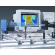
北京欧兰科技发展有限公司为您提供《新型波中新型波的产生检测方案(粒子图像测速)》,该方案主要用于其他中新型波的产生检测,参考标准--,《新型波中新型波的产生检测方案(粒子图像测速)》用到的仪器有德国LaVision PIV/PLIF粒子成像测速场仪、Imager sCMOS PIV相机、PLIF平面激光诱导荧光火焰燃烧检测系统
推荐专场


相关方案
更多
该厂商其他方案
更多