旋转流体中惯性波束的黏滞扩散检测方案(粒子图像测速)

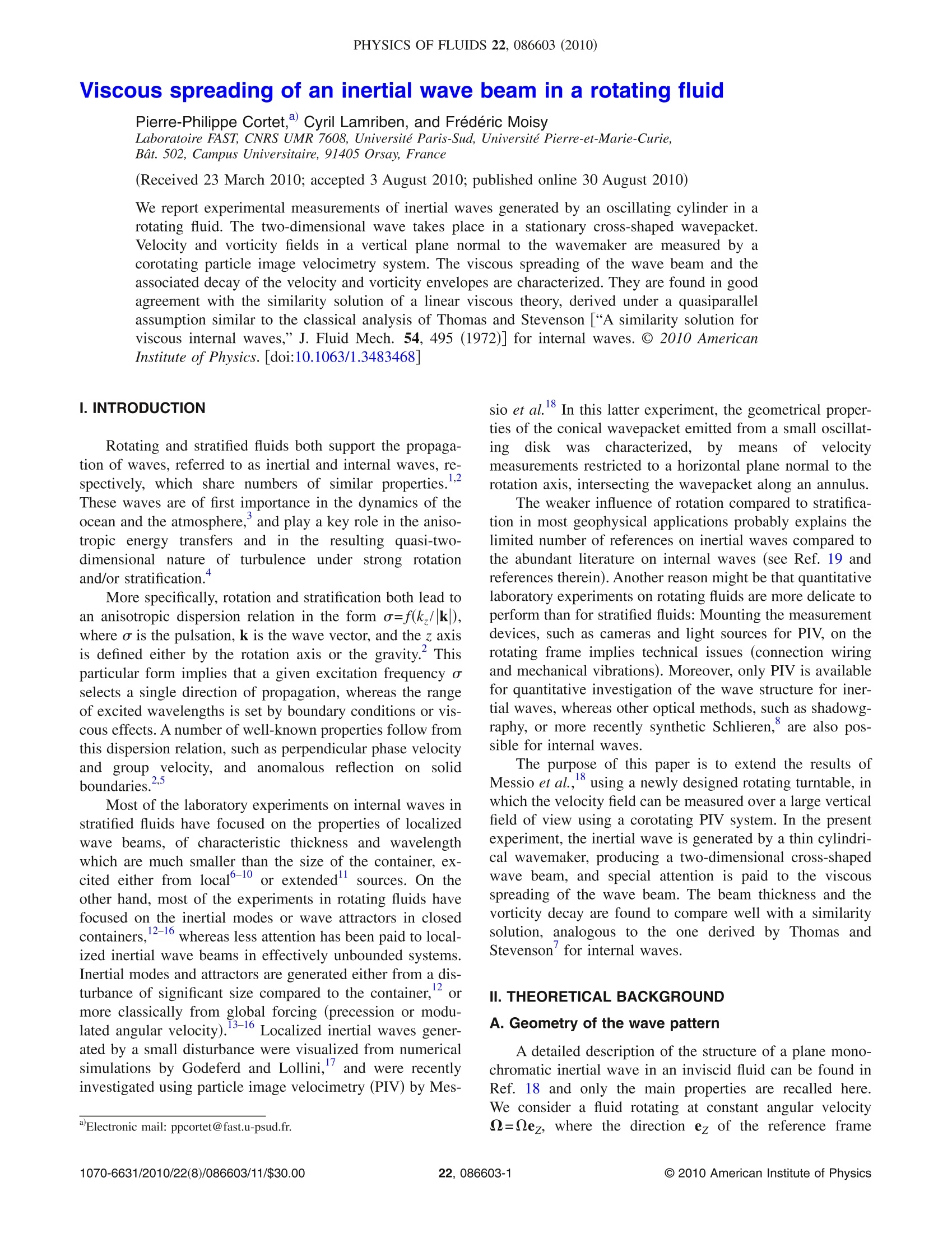
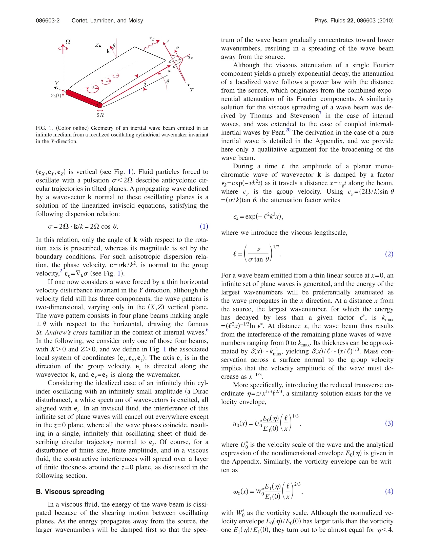
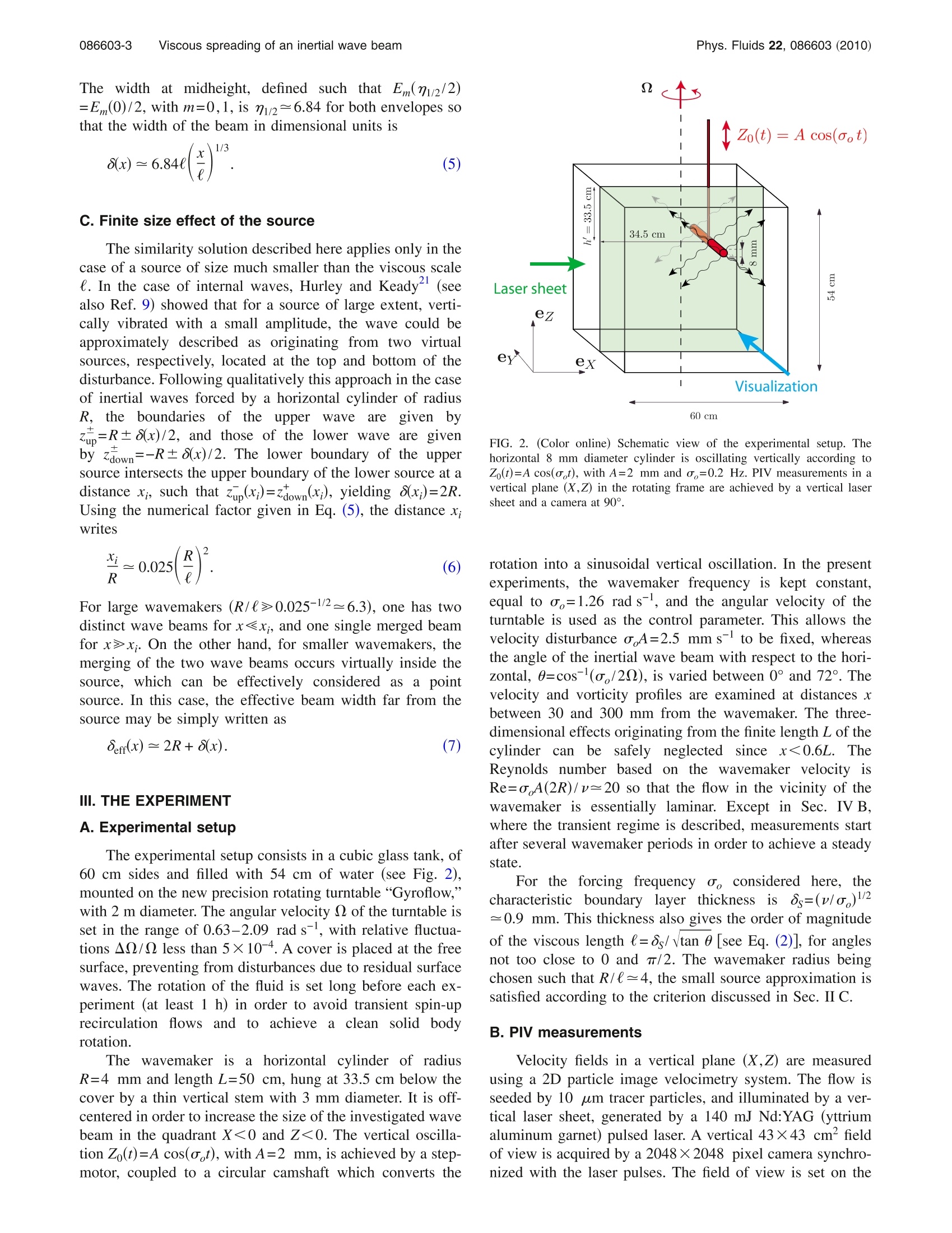
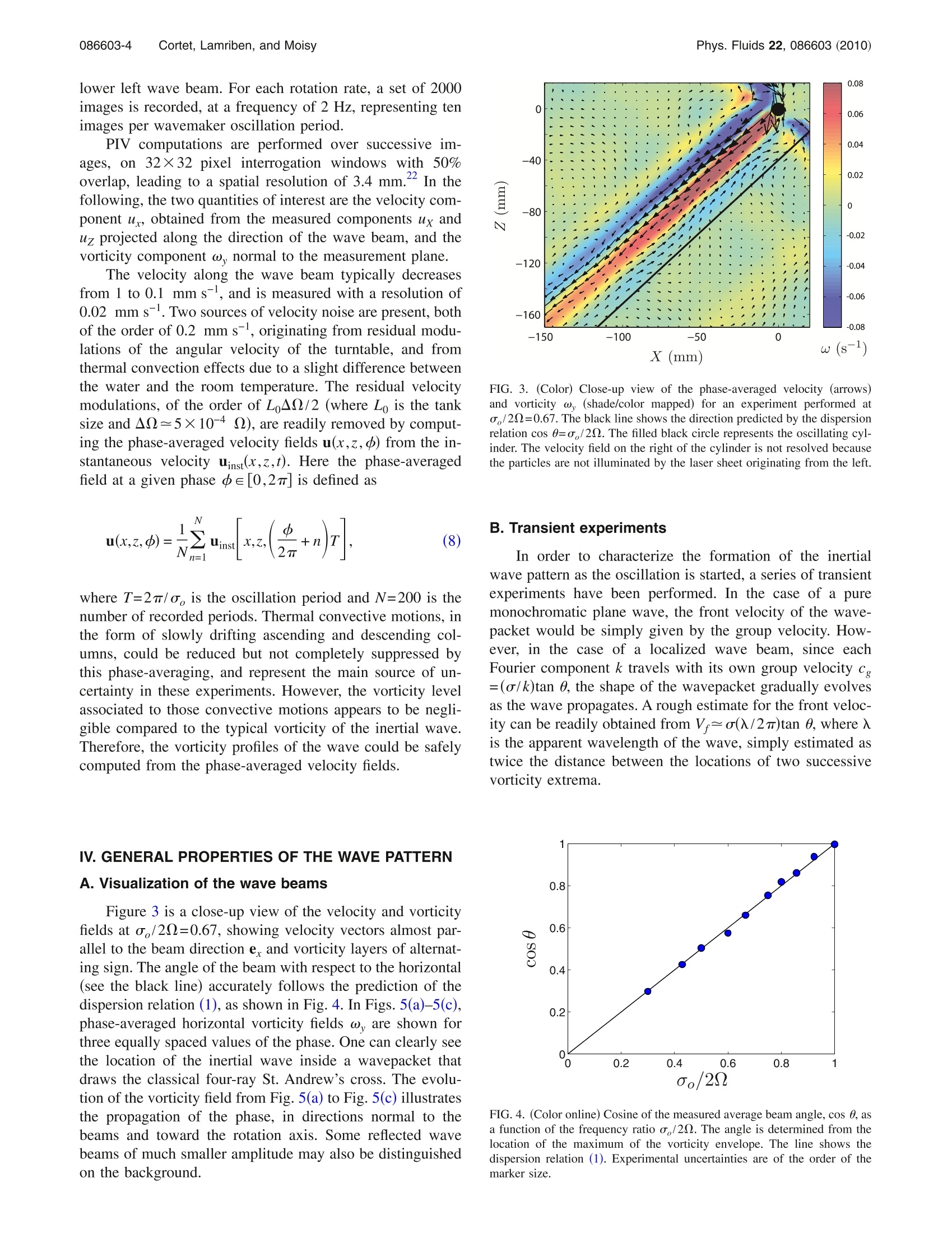
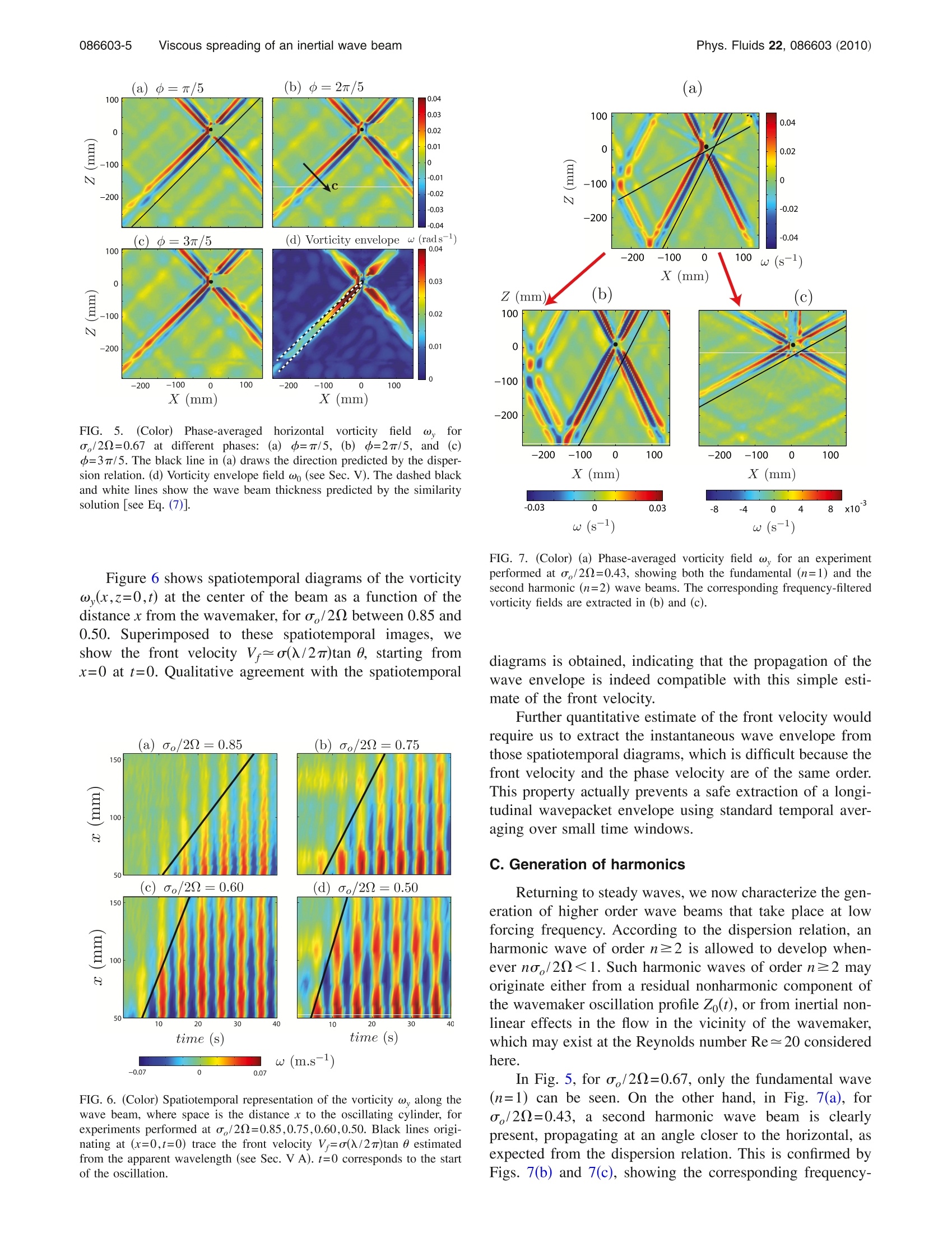
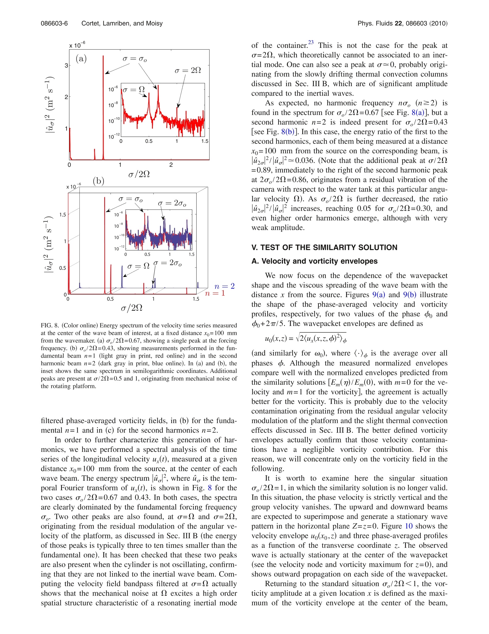
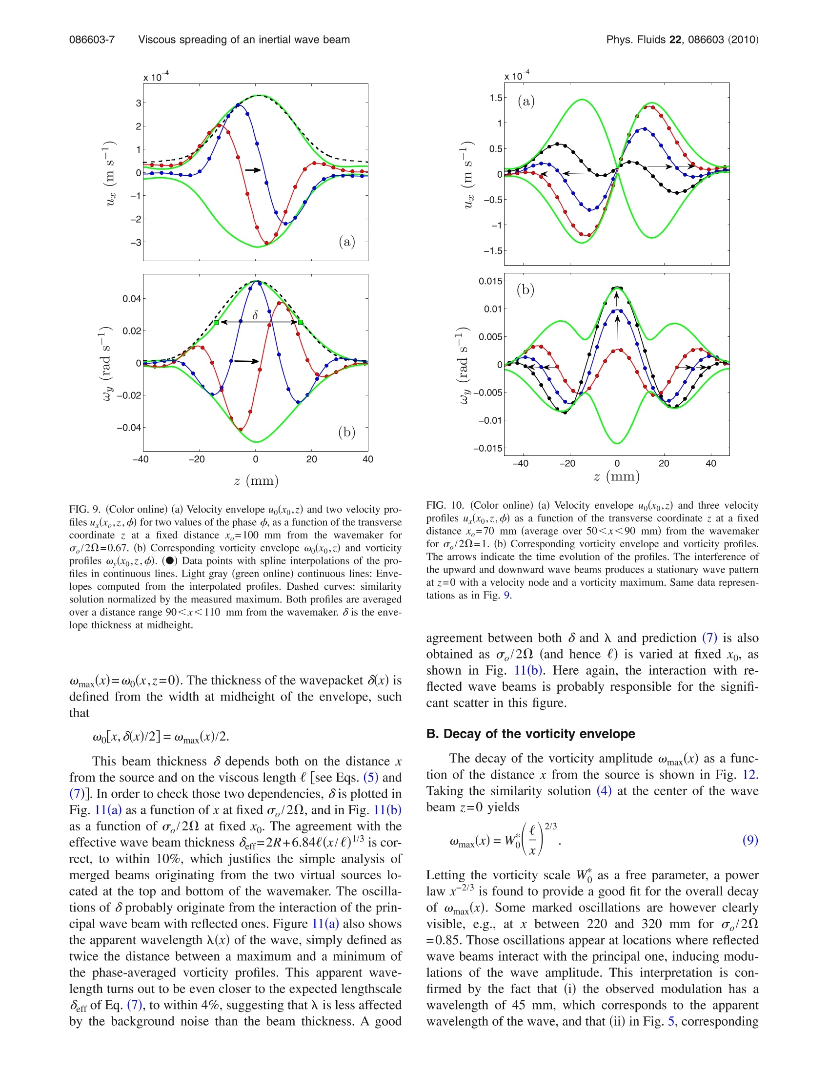
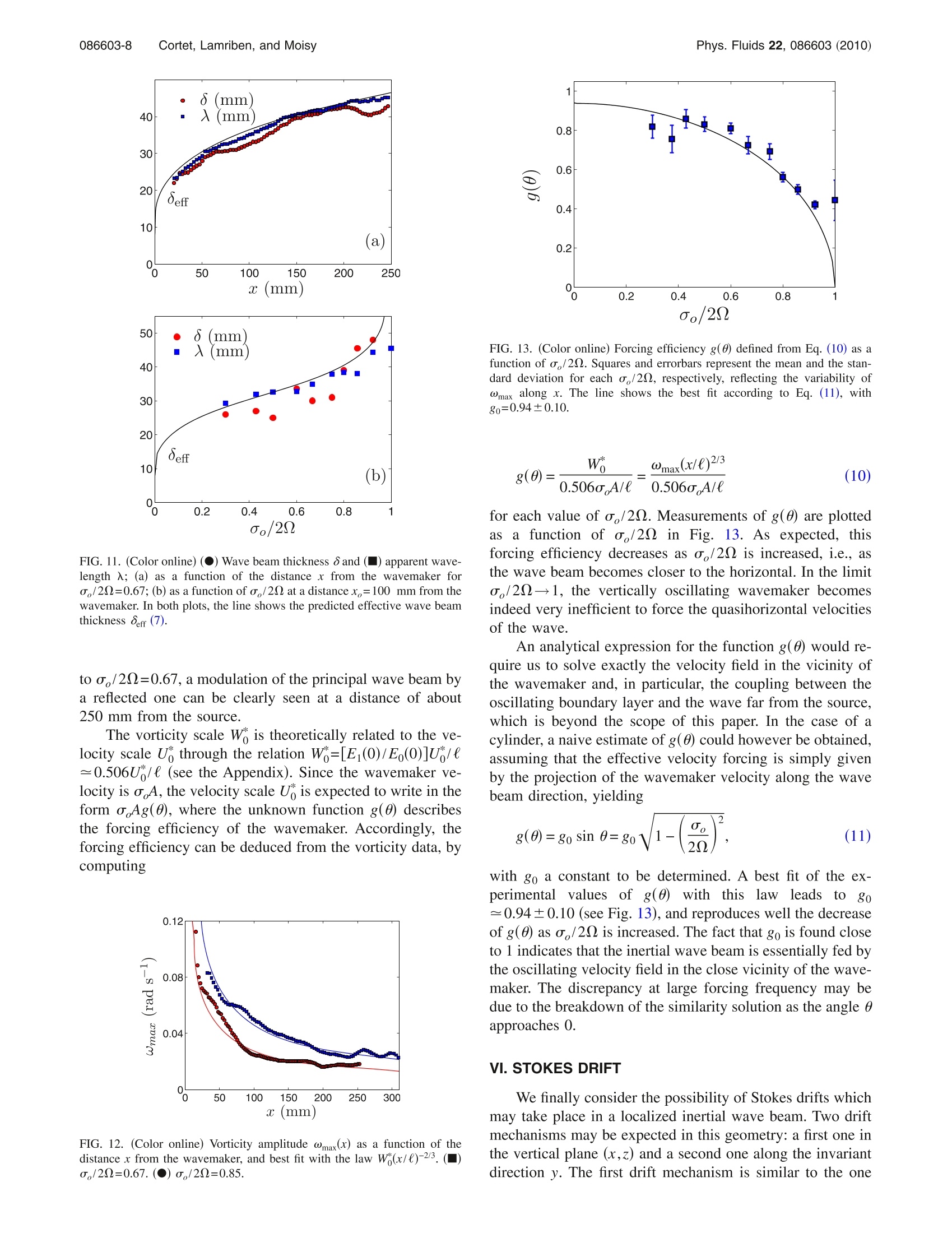
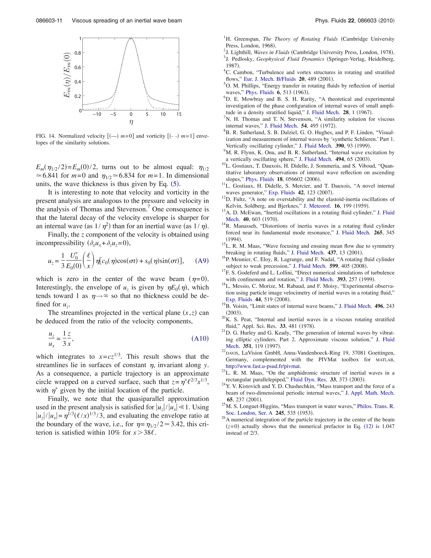
PHYSICS OF FLUIDS 22， 086603 (2010) Phys. Fluids 22， 086603 (2010)086603-2 Viscous spreading of an inertial wave beam in a rotating fluid Pierre-Philippe Cortet， Cyril Lamriben， and Frederic Moisy Laboratoire FAST， CNRS UMR 7608， Universite Paris-Sud， Universite Pierre-et-Marie-Curie， Bat. 502， Campus Universitaire， 91405 Orsay， France (Received 23 March 2010； accepted 3 August 2010； published online 30 August 2010) We report experimental measurements of inertial waves generated by an oscillating cylinder in arotating fluid. The two-dimensional wave takes place in a stationary cross-shaped wavepacket.Velocity and vorticity fields in a vertical plane normal to the wavemaker are measured by acorotating particle image velocimetry system. The viscous spreading of the wave beam and theassociated decay of the velocity and vorticity envelopes are characterized. They are found in goodagreement with the similarity solution of a linear viscous theory， derived under a quasiparallelassumption similar to the classical analysis of Thomas and Stevenson “A similarity solution forviscous internal waves，”J. Fluid Mech. 54， 495 (1972)] for internal waves. @ 2010 AmericanInstitute of Physics.[doi：10.1063/1.3483468 I. INTRODUCTION Rotating and stratified fluids both support the propaga-tion of waves， referred to as inertial and internal waves， re-spectively， which share numbers of similar properties.These waves are of first importance in the dynamics of theocean and the atmosphere，and play a key role in the aniso-tropic energy transfers and in the resulting quasi-two-dimensional nature of turbulence under strong rotationand/or stratification. More specifically， rotation and stratification both lead toan anisotropic dispersion relation in the form o=f(k/ k)，where o is the pulsation， k is the wave vector， and the z axisis defined either by the rotation axis or the gravity.Thisparticular form implies that a given excitation frequency oselects a single direction of propagation， whereas the rangeof excited wavelengths is set by boundary conditions or vis-cous effects. A number of well-known properties follow fromthis dispersion relation， such as perpendicular phase velocityand group velocity， and anomalous reflection on solidboundaries.2 Most of the laboratory experiments on internal waves instratified fluids have focused on the properties of localizedwave beams， of characteristic thickness and wavelengthwhich are much smaller than the size of the container， ex-cited either from local6-10or extended sources. On theother hand， most of the experiments in rotating fluids havefocused on the inertial modes or wave attractors in closedcontainers，12-16 whereas less attention has been paid to local-ized inertial wave beams in effectively unbounded systems.Inertial modes and attractors are generated either from a dis-turbance of significant size comp12ared to the container，ormore classically from global forcing (precession or modu-lated angular velocity).13-16 Localized inertial waves gener-ated by a small disturbance were visualized from numericalsimulations by Godeferd and Lollini， and were recentlyinvestigated using particle image velocimetry (PIV) by Mes- sio et a1.18 In this latter experiment， the geometrical proper-ties of the conical wavepacket emitted from a small oscillat-ing disk was characterized.byymeans ofvelocitymeasurements restricted to a horizontal plane normal to therotation axis， intersecting the wavepacket along an annulus. The weaker influence of rotation compared to stratifica-tion in most geophysical applications probably explains thelimited number of references on inertial waves compared tothe abundant literature on internal waves (see Ref. 19 andreferences therein). Another reason might be that quantitativelaboratory experiments on rotating fluids are more delicate toperform than for stratified fluids： Mounting the measurementdevices， such as cameras and light sources for PIV， on therotating frame implies technical issues (connection wiringand mechanical vibrations). Moreover， only PIV is availablefor quantitative investigation of the wave structure for iner-tial waves， whereas other optical methods， such as shadowg-raphy， or more recently synthetic Schlieren，°' are also pos-sible for internal waves. The purpose of this paper is to extend the results ofMessio et al.， using a newly designed rotating turntable， inwhich the velocity field can be measured over a large verticalfield of view using a corotating PIV system. In the presentexperiment， the inertial wave is generated by a thin cylindri-cal wavemaker， producing a two-dimensional cross-shapedwave beam， and special attention is paid to the viscousspreading of the wave beam. The beam thickness and thevorticity decay are found to compare well with a similaritysolution， analogous to the one derived by Thomas andStevenson’ for internal waves. II.THEORETICAL BACKGROUND A. Geometry of the wave pattern A detailed description of the structure of a plane mono-chromatic inertial wave in an inviscid fluid can be found inRef. 18 and only the main properties are recalled here.We consider a fluid rotating at constant angular velocity=Qez， where the direction ez of the reference frame 2R FIG. 1. (Color online) Geometry of an inertial wave beam emitted in aninfinite medium from a localized oscillating cylindrical wavemaker invariantin the Y-direction. (ex，ey，ez) is vertical (see Fig. 1). Fluid particles forced tooscillate with a pulsation o<20 describe anticyclonic cir-cular trajectories in tilted planes. A propagating wave definedby a wavevector k normal to these oscillating planes is asolution of the linearized inviscid equations， satisfying thefollowing dispersion relation： In this relation， only the angle of k with respect to the rota-tion axis is prescribed， whereas its magnitude is set by theboundary conditions. For such anisotropic dispersion rela-tion， the phase velocity， c=ok/k²， is normal to the groupvelocity，cg=Vko (see Fig. 1). If one now considers a wave forced by a thin horizontalvelocity disturbance invariant in the Y direction， although thevelocity field still has three components， the wave pattern istwo-dimensional， varying only in the (X，Z) vertical plane.The wave pattern consists in four plane beams making angle±0 with respect to the horizontal， drawing the famousSt. Andrew's cross familiar in the context of internal waves.In the following， we consider only one of those four beams，with X>0 and Z>0， and we define in Fig. 1 the associatedlocal system of coordinates (e.，e，，e)： The axis e， is in thedirection of the group velocity， e is directed along thewavevector k， and e，=ey is along the wavemaker. Considering the idealized case of an infinitely thin cyl-inder oscillating with an infinitely small amplitude (a Diracdisturbance)， a white spectrum of wavevectors is excited， allaligned with e. In an inviscid fluid， the interference of thisinfinite set of plane waves will cancel out everywhere exceptin the z=0 plane， where all the wave phases coincide， result-ing in a single， infinitely thin oscillating sheet of fluid de-scribing circular trajectory normal to e . Of course， for adisturbance of finite size， finite amplitude， and in a viscousfluid， the constructive interferences will spread over a layerof finite thickness around the z=0 plane， as discussed in thefollowing section. B. Viscous spreading In a viscous fluid， the energy of the wave beam is dissi-pated because of the shearing motion between oscillatingplanes. As the energy propagates away from the source， thelarger wavenumbers will be damped first so that the spec- trum of the wave beam gradually concentrates toward lowerwavenumbers， resulting in a spreading of the wave beamaway from the source. Although the viscous attenuation of a single Fouriercomponent yields a purely exponential decay，the attenuationof a localized wave follows a power law with the distancefrom the source， which originates from the combined expo-nential attenuation of its Fourier components. A similaritysolution for the viscous spreading of a wave beam was de-rived by Thomas and Stevenson’’ in the case of internalwaves， and was extended to the case of coupled internal-inertial waves by Peat. The derivation in the case of a pureinertial wave is detailed in the Appendix， and we providehere only a qualitative argument for the broadening of thewave beam. During a time t， the amplitude of a planar mono-chromatic wave of wavevector k is damped by a factore=exp(-uk’t) as it travels a distance x=ct along the beam，where c is the group velocity. Using c=(20/k)sin 0=(o/k)tan 0， the attenuation factor writes where we introduce the viscous lengthscale， For a wave beam emitted from a thin linear source at x=0， aninfinite set of plane waves is generated， and the energy of thelargest wavenumbers will be preferentially attenuated asthe wave propagates in the x direction. At a distance x fromthe source， the largest wavenumber， for which the energyhas decayed by lessthani a given factor e， is kmax=(C2x)-1/3ln e*. At distance x， the wave beam thus resultsfrom the interference of the remaining plane waves of wave-numbers ranging from0 to kmax. Its thickness can be approxi-mated by 8(x)~kax， yielding 8(x)/e~(x/e)1/3. Mass con-servation across a surface normal to the group velocityimplies that the velocity amplitude of the wave must de-crease as x-1/3 More specifically， introducing the reduced transverse co-ordinate n=z/x1/3e2/3， a similarity solution exists for the ve-locity envelope， where U is the velocity scale of the wave and the analyticalexpression of the nondimensional envelope Eo(D) is given inthe Appendix. Similarly， the vorticity envelope can be writ-ten as with W as the vorticity scale. Although the normalized ve-locity envelope E()/E (0) has larger tails than the vorticityone E(D)/E(0)， they turn out to be almost equal for n<4. The width at midheight， defined such that Em(71/2/2)=Em(0)/2， with m=0，1， is?1/2~6.84 for both envelopes sothat the width of the beam in dimensional units is C. Finite size effect of the source The similarity solution described here applies only in thecase of a source of size much smaller than the viscous scalee. In the case of internal waves， Hurley and Keady(seealso Ref. 9) showed that for a source of large extent， verti-cally vibrated with a small amplitude， the wave could beapproximately described as originating from two virtualsources， respectively， located at the top and bottom of thedisturbance.Following qualitatively this approach in the caseof inertial waves forced by a horizontal cylinder of radiusR， the boundaries of the upper waveareegivenbyz=R±8(x)/2， and those of the lower wave are givenby zaown=-R±8(x)/2. The lower boundary of the uppersource intersects the upper boundary of the lower source at adistance x， such that zup(x；)=zdown(x；)， yielding 8(x；)=2R.Using the numerical factor given in Eq. (5)， the distance x；writes For large wavemakers (R/(>0.025-1/2=6.3)， one has twodistinct wave beams for xx. On the other hand， for smaller wavemakers， themerging of the two wave beams occurs virtually inside thesource， which can be effectively considered as a pointsource. In this case， the effective beam width far from thesource may be simply written as III.THE EXPERIMENT A. Experimental setup The experimental setup consists in a cubic glass tank， of60 cm sides and filled with 54 cm of water (see Fig. 2)，mounted on the new precision rotating turntable“Gyroflow，”with 2 m diameter. The angular velocity of the turntable isset in the range of 0.63-2.09 rad s-， with relative fluctua-tions A0/ less than 5×10-4. A cover is placed at the freesurface， preventing from disturbances due to residual surfacewaves. The rotation of the fluid is set long before each ex-periment (at least 1 h) in order to avoid transient spin-uprecirculation flows and to achieve a clean solid bodyrotation. The wavemaker issahorizontal cylinder of radiusR=4 mm and length L=50 cm， hung at 33.5 cm below thecover by a thin vertical stem with 3 mm diameter. It is off-centered in order to increase the size of the investigated wavebeam in the quadrant X<0 and Z<0. The vertical oscilla-tion Zo(t)=A cos(o t)， with A=2 mm， is achieved by a step-motor， coupled to a circular camshaft which converts the FIG. 2. (Color online) Schematic view of the experimental setup. Thehorizontal 8 mm diameter cylinder is oscillating vertically according toZ (t)=A cos(o，t)， with A=2 mm and o，=0.2 Hz. PIV measurements in avertical plane (X，Z) in the rotating frame are achieved by a vertical lasersheet and a camera at 90°. rotation into a sinusoidal vertical oscillation. In the presentexperiments， the wavemaker frequency is kept constant，equal to o=1.26 rad s-， and the angular velocity of theturntable is used as the control parameter. This allows thevelocity disturbance oA=2.5 mm s-l to be fixed， whereasthe angle of the inertial wave beam with respect to the hori-zontal， 0=cos (o，/22)， is varied between 0° and 72°. Thevelocity and vorticity profiles are examined at distances xbetween 30 and 300 mm from the wavemaker. The three-dimensional effects originating from the finite length L of thecylinder canbe safely neglected since x<0.6L. TheReynolds number based on the wavemaker velocity isRe=o，A(2R)/v=20 so that the flow in the vicinity of thewavemaker is essentially laminar. Except in Sec. IV B，where the transient regime is described， measurements startafter several wavemaker periods in order to achieve a steadystate. Fo he forcing frequencyy aa，。 cconsidered here， thecharacteristic boundary layer thicknessis1S8s=(v/o)1/2=0.9 mm. This thickness also gives the order of magnitudeof the viscous length e=8s/ √tan 0 [see Eq. (2)]， for anglesnot too close to 0 and m/2. The wavemaker radius beingchosen such that R/l=4， the small source approximation issatisfied according to the criterion discussed in Sec. II C. B. PIV measurements Velocity fields in a vertical plane (X，Z) are measuredusing a 2D particle image velocimetry system. The flow isseeded by 10 um tracer particles， and illuminated by a ver-tical laser sheet， generated by a 140 mJ Nd：YAG (yttriumaluminum garnet) pulsed laser. A vertical 43×43 cm² fieldof view is acquired by a 2048×2048 pixel camera synchro-nized with the laser pulses. The field of view is set on the lower left wave beam. For each rotation rate， a set of 2000images is recorded， at a frequency of 2 Hz， representing tenimages per wavemaker oscillation period. PIV computations are performed over successive im-ages， on 32×32 pixel interrogation windows with 50%overlap， leading to a spatial resolution of 3.4 mm." In thefollowing， the two quantities of interest are the velocity com-ponent uy， obtained from the measured components uy anduz projected along the direction of the wave beam， and thevorticity component w， normal to the measurement plane. The velocity along the wave beam typically decreasesfrom 1 to 0.1 mm s-， and is measured with a resolution of0.02 mm s-. Two sources of velocity noise are present， bothof the order of 0.2 mm s， originating from residual modu-lations of the angular velocity of the turntable， and fromthermal convection effects due to a slight difference betweenthe water and the room temperature. The residual velocitymodulations， of the order of LA0/2 (where Lo is the tanksize and 0=5×10-4a)， are readily removed by comput-ing the phase-averaged velocity fields u(x，z，p) from the in-stantaneous velocity uinst(x，z，t). Here the phase-averagedfield at a given phase 中e [0，2m] is defined as where T=2n/a， is the oscillation period and N=200 is thenumber of recorded periods. Thermal convective motions， inthe form of slowly drifting ascending and descending col-umns， could be reduced but not completely suppressed bythis phase-averaging， and represent the main source of un-certainty in these experiments. However， the vorticity levelassociated to those convective motions appears to be negli-gible compared to the typical vorticity of the inertial wave.Therefore， the vorticity profiles of the wave could be safelycomputed from the phase-averaged velocity fields. |V. GENERAL PROPERTIES OF THE WAVE PATTERNA. Visualization of the wave beams Figure 3 is a close-up view of the velocity and vorticityfields at o/20=0.67， showing velocity vectors almost par-allel to the beam direction e， and vorticity layers of alternat-ing sign. The angle of the beam with respect to the horizontal(see the black line) accurately follows the prediction of thedispersion relation (1)， as shown in Fig. 4. In Figs. 5(a)-5(c)，phase-averaged horizontal vorticity fields ω， are shown forthree equally spaced values of the phase. One can clearly seethe location of the inertial wave inside a wavepacket thatdraws the classical four-ray St. Andrew’s cross. The evolu-tion of the vorticity field from Fig. 5(a) to Fig.5(c) illustratesthe propagation of the phase， in directions normal to thebeams and toward the rotation axis. Some reflected wavebeams of much smaller amplitude may also be distinguishedon the background. FIG. 3. (Color) Close-up view of the phase-averaged velocity (arrows)and vorticity w (shade/color mapped) for an experiment performed ata，/20=0.67. The black line shows the direction predicted by the dispersionrelation cos 0=o，/20. The filled black circle represents the oscillating cyl-inder. The velocity field on the right of the cylinder is not resolved becausethe particles are not illuminated by the laser sheet originating from the left. B. Transient experiments In order to characterize the formation of the inertialwave pattern as the oscillation is started， a series of transientexperiments have been performed. In the case of a puremonochromatic plane wave， the front velocity of the wave-packet would be simply given by the group velocity. How-ever， in the case of a localized wave beam， since eachFourier component k travels with its own group velocity c=(o/k)tan 0，the shape of the wavepacket gradually evolvesas the wave propagates. A rough estimate for the front veloc-ity can be readily obtained from V=o()/2m)tan 0， where 入is the apparent wavelength of the wave， simply estimated astwice the distance between the locations of two successivevorticity extrema. FIG. 4. (Color online) Cosine of the measured average beam angle， cos 0， asa function of the frequency ratio a/2Q. The angle is determined from thelocation of the maximum of the vorticity envelope. The line shows thedispersion relation (1). Experimental uncertainties are of the order of themarker size. FIG. 5.(Color))1Phase-averageddhorizontalvorticityfield 'yforo，/20=0.67 at different phases： (a)+=m/5， (b) d=2m/5， and (c)d=3m/5. The black line in (a) draws the direction predicted by the disper-sion relation. (d) Vorticity envelope field wo (see Sec. V). The dashed blackand white lines show the wave beam thickness predicted by the similaritysolution [see Eq. (7)]. Figure 6 shows spatiotemporal diagrams of the vorticityω，(x，z=0，t) at the center of the beam as a function of thedistance x from the wavemaker， for o，/20 between 0.85 and0.50. Superimposed to these spatiotemporal images，weshow the front velocityV=o(二/2m)tan O， starting fromx=0 at t=0. Qualitative agreement with the spatiotemporal FIG. 6. (Color) Spatiotemporal representation of the vorticity ω，along thewave beam， where space is the distance x to the oscillating cylinder， forexperiments performed at o，/22=0.85，0.75，0.60，0.50. Black lines origi-nating at (x=0，t=0) trace the front velocity V=o(/2n)tan 0 estimatedfrom the apparent wavelength (see Sec. VA). t=0 corresponds to the startof the oscillation. (a) Z (mm) (b) (c) FIG. 7. (Color) (a) Phase-averaged vorticity field w， for an experimentperformed at r/20=0.43， showing both the fundamental (n=1) and thesecond harmonic (n=2) wave beams. The corresponding frequency-filteredvorticity fields are extracted in (b) and (c). diagrams is obtained， indicating that the propagation of thewave envelope is indeed compatible with this simple esti-mate of the front velocity. Further quantitative estimate of the front velocity wouldrequire us to extract the instantaneous wave envelope fromthose spatiotemporal diagrams， which is difficult because thefront velocity and the phase velocity are of the same order.This property actually prevents a safe extraction of a longi-tudinal wavepacket envelope using standard temporal aver-aging over small time windows. C. Generation of harmonics Returning to steady waves， we now characterize the gen-eration of higher order wave beams that take place at lowforcing frequency. According to the dispersion relation， anharmonic wave of order n2 is allowed to develop when-ever no，/20<1. Such harmonic waves of order n≥2 mayoriginate either from a residual nonharmonic component ofthe wavemaker oscillation profile Z (t)， or from inertial non-linear effects in the flow in the vicinity of the wavemaker，which may exist at the Reynolds number Re=20 consideredhere. In Fig. 5， forr/20=0.67， only the fundamental wave(n=1) can be seen. On the other hand， in Fig. 7(a)， foro，/2Q=0.43， a second harmonic wave beam is clearlypresent， propagating at an angle closer to the horizontal， asexpected from the dispersion relation. This is confirmed byFigs. 7(b) and 7(c)， showing the corresponding frequency- x10 in =2 0/22 FIG. 8. (Color online) Energy spectrum of the velocity time series measuredat the center of the wave beam of interest， at a fixed distance xo=100 mmfrom the wavemaker. (a)o，/20=0.67， showing a single peak at the forcingfrequency. (b)o /20=0.43， showing measurements performed in the fun-damental beam n=1 (light gray in print， red online) and in the secondharmonic beam n=2 (dark gray in print， blue online). In (a) and (b)， theinset shows the same spectrum in semilogarithmic coordinates.Additionalpeaks are present at o/20=0.5 and 1， originating from mechanical noise ofthe rotating platform. filtered phase-averaged vorticity fields， in (b) for the funda-mental n=1 and in (C) for the second harmonicsn=2. In order to further characterize this generation of har-monics， we have performed a spectral analysis of the timeseries of the longitudinal velocity uy(t)， measured at a givendistance xo=100 mm from the source， at the center of eachwave beam. The energy spectrum a 2， where u is the tem-poral Fourier transform of u (t)， is shown in Fig. 8 for thetwo cases o，/20=0.67 and 0.43. In both cases， the spectraare clearly dominated by the fundamental forcing frequencyo. Two other peaks are also found， at o=0 and o=20，originating from the residual modulation of the angular ve-locity of the platform， as discussed in Sec. III B (the energyof those peaks is typically three to ten times smaller than thefundamental one). It has been checked that these two peaksare also present when the cylinder is not oscillating， confirm-ing that they are not linked to the inertial wave beam. Com-puting the velocity field bandpass filtered at o=2 actuallyshows that the mechanical noise at excites a high orderspatial structure characteristic of a resonating inertial mode of the container.3 This is not the case for the peak ato=2Q， which theoretically cannot be associated to an iner-tial mode. One can also see a peak at o=0，probably origi-nating from the slowly drifting thermal convection columnsdiscussed in Sec. III B， which are of significant amplitudecompared to the inertial waves. As expected， no harmonic frequency no， (n≥2) isfound in the spectrum for o /2=0.67 [see Fig.8(a)]， but asecond harmonic n=2 is indeed present for o/20=0.43[see Fig. 8(b)]. In this case， the energy ratio of the first to thesecond harmonics， each of them being measured at a distancexo=100 mm from the source on the corresponding beam， is|u2o2/a2=0.036. (Note that the additional peak at o/2=0.89，immediately to the right of the second harmonic peakat 2o，/20=0.86， originates from a residual vibration of thecamera with respect to the water tank at this particular angu-lar velocity ). As o/20 is further decreased， the ratiou202/a2 increases， reaching 0.05 for o /22=0.30， andeven higher order harmonics emerge， although with veryweak amplitude. V. TEST OF THE SIMILARITY SOLUTION A. Velocity and vorticity envelopes We now focus on the dependence of the wavepacketshape and the viscous spreading of the wave beam with thedistance x from the source. Figures 9(a) and 9(b) illustratethe shape of the phase-averaged velocity and vorticityprofiles， respectively， for two values of the phase do and中o+2m/5. The wavepacket envelopes are defined as (and similarly for wo)， where(.)is the average over allphasesS d(. Although the measured normalized envelopescompare well with the normalized envelopes predicted fromthe similarity solutions [Em()/Em(0)， with m=0 for the ve-locity and m=1 for the vorticity]， the agreement is actuallybetter for the vorticity. This is probably due to the velocitycontamination originating from the residual angular velocitymodulation of the platform and the slight thermal convectioneffects discussed in Sec. III B. The better defined vorticityenvelopes actually confirm that those velocity contamina-tions have a negligible vorticity contribution. For thisreason， we will concentrate only on the vorticity field in thefollowing. It i1sSworth to examine here the singular situationo，/20=1， in which the similarity solution is no longer valid.In this situation， the phase velocity is strictly vertical and thegroup velocity vanishes. The upward and downward beamsare expected to superimpose and generate a stationary wavepattern in the horizontal plane Z=z=0. Figure 10 shows thevelocity envelope uo(xo，z) and three phase-averaged profilesas a function of the transverse coordinate z. The observedwave is actually stationary at the center of the wavepacket(see the velocity node and vorticity maximum for z=0)， andshows outward propagation on each side of the wavepacket. Returning to the standard situation o，/20<1， the vor-ticity amplitude at a given location x is defined as the maxi-mum of the vorticity envelope at the center of the beam， FIG.9. (Color online) (a) Velocity envelope uo(xo，z) and two velocity pro-files uy(xo，z，d) for two values of the phase d， as a function of the transversecoordinate z at a fixed distance x =100 mm from the wavemaker foro，/20=0.67. (b) Corresponding vorticity envelope wo(xo，z) and vorticityprofiles ω，(xo，z，d). () Data points with spline interpolations of the pro-files in continuous lines. Light gray (green online) continuous lines： Enve-lopes computed from the interpolated profiles. Dashed curves： similaritysolution normalized by the measured maximum. Both profiles are averagedover a distance range 90