液体中三维贯穿度和速度分布检测方案(粒子图像测速)

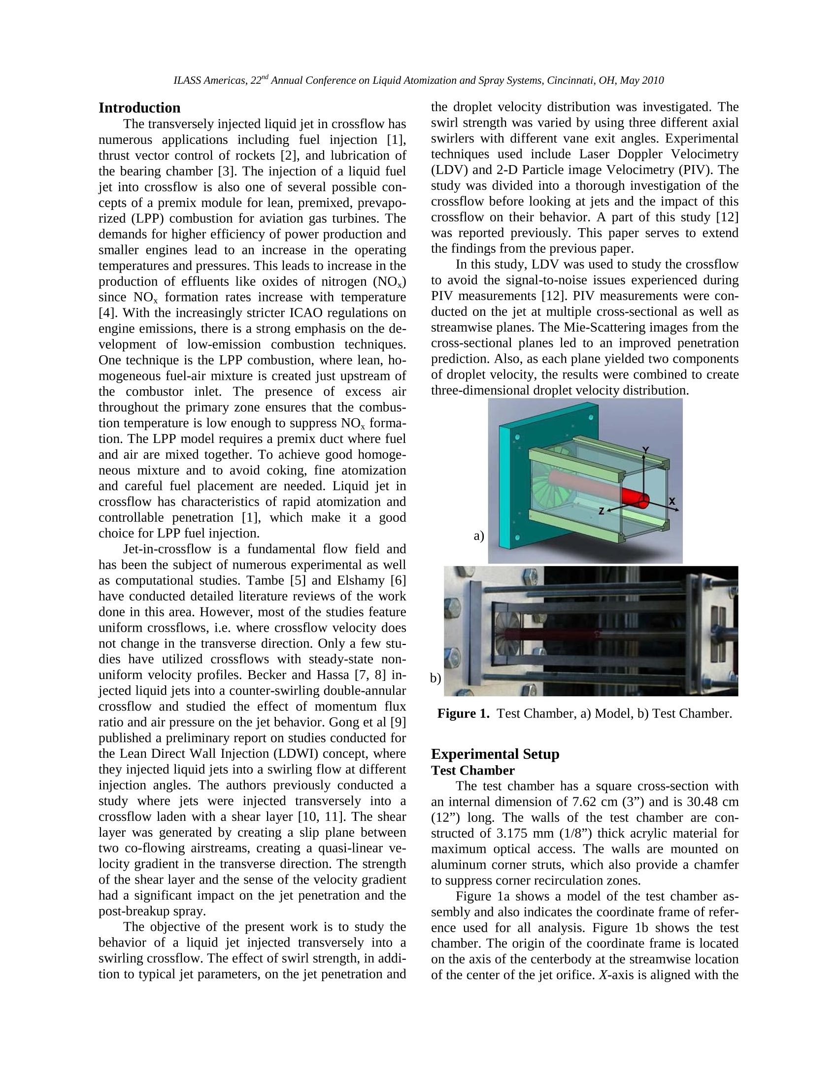
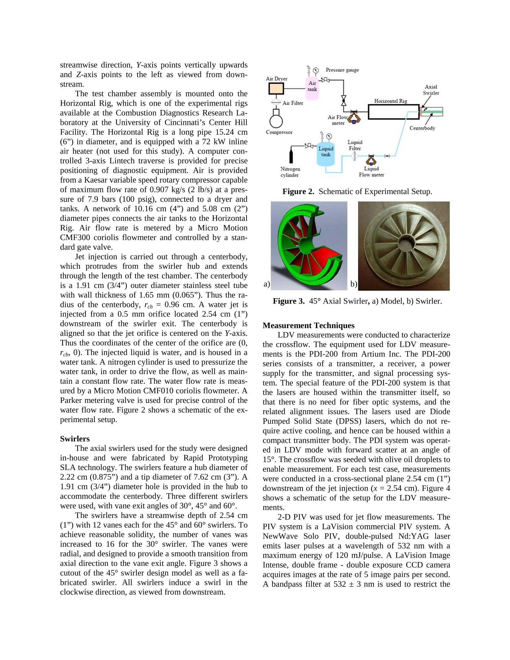
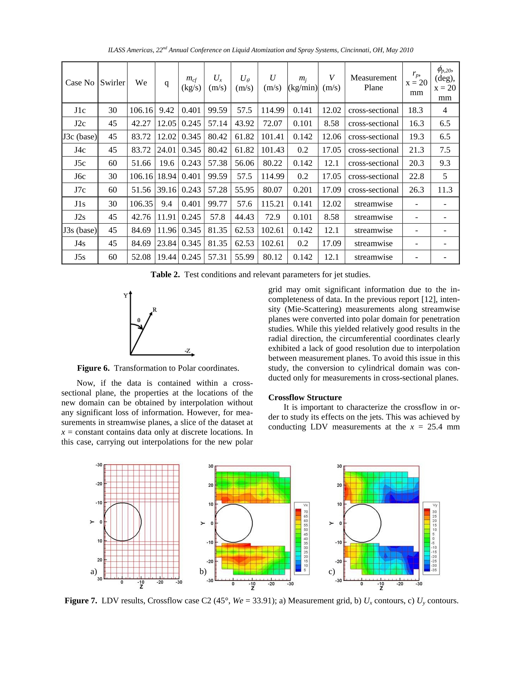
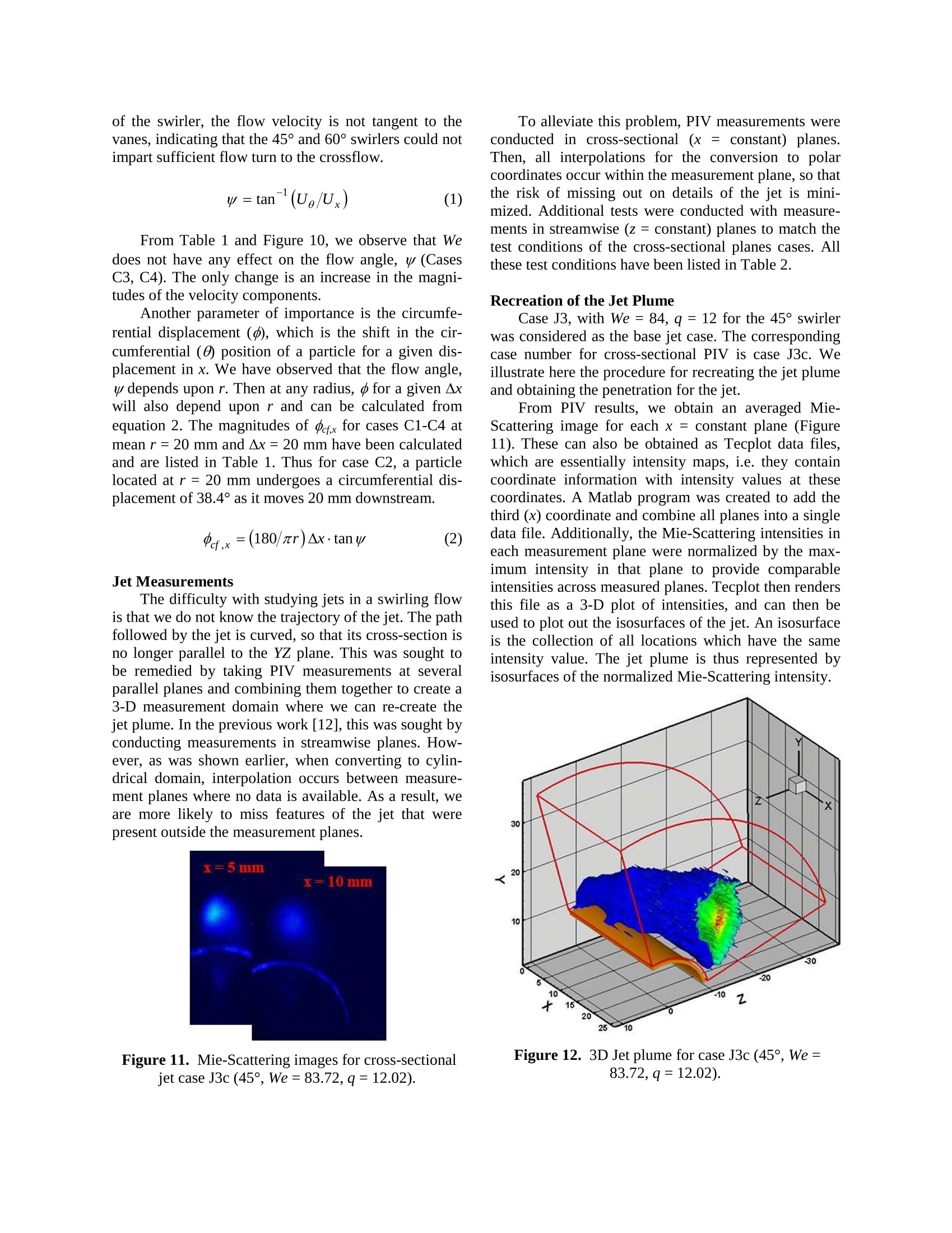
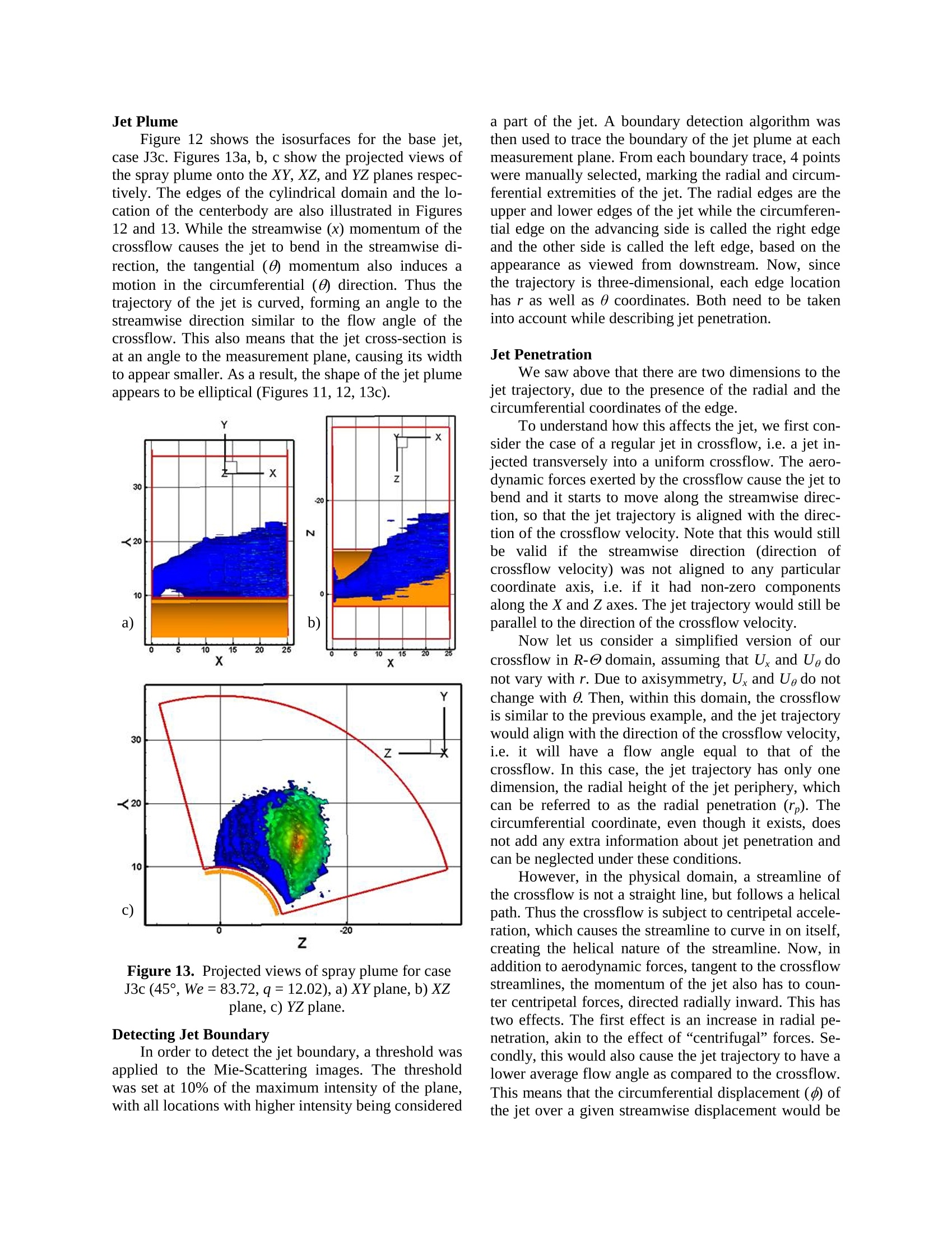
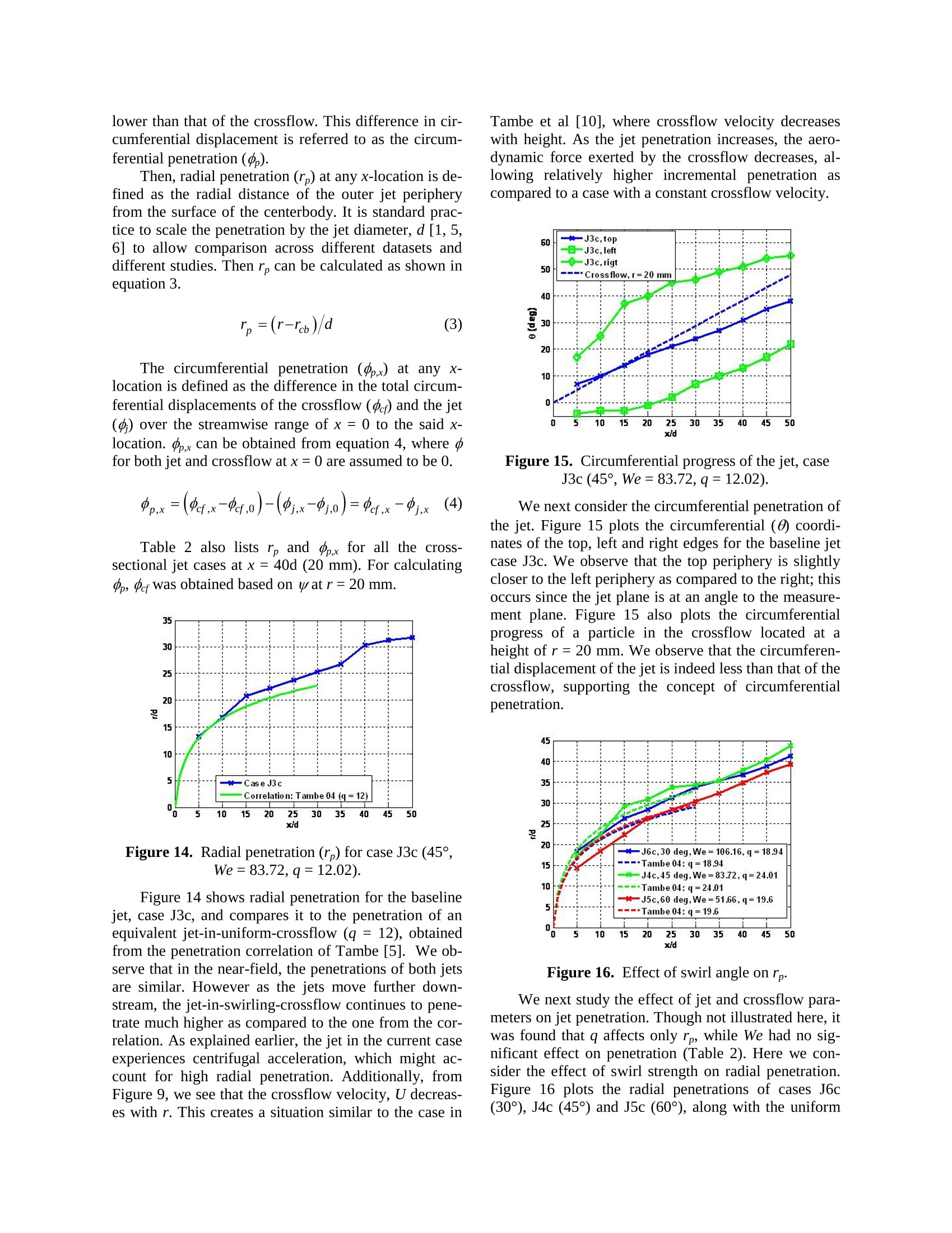
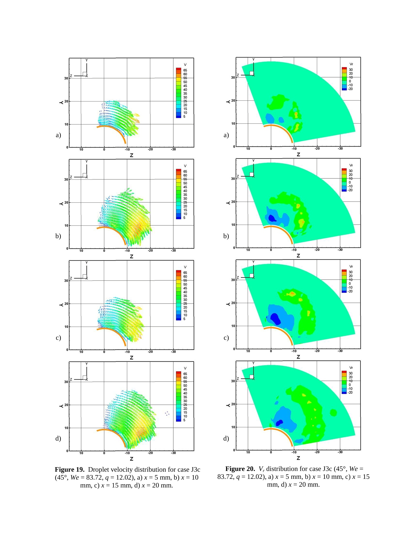
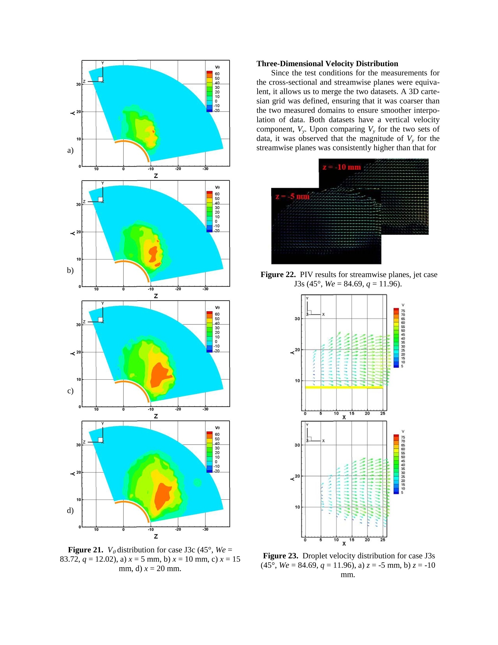
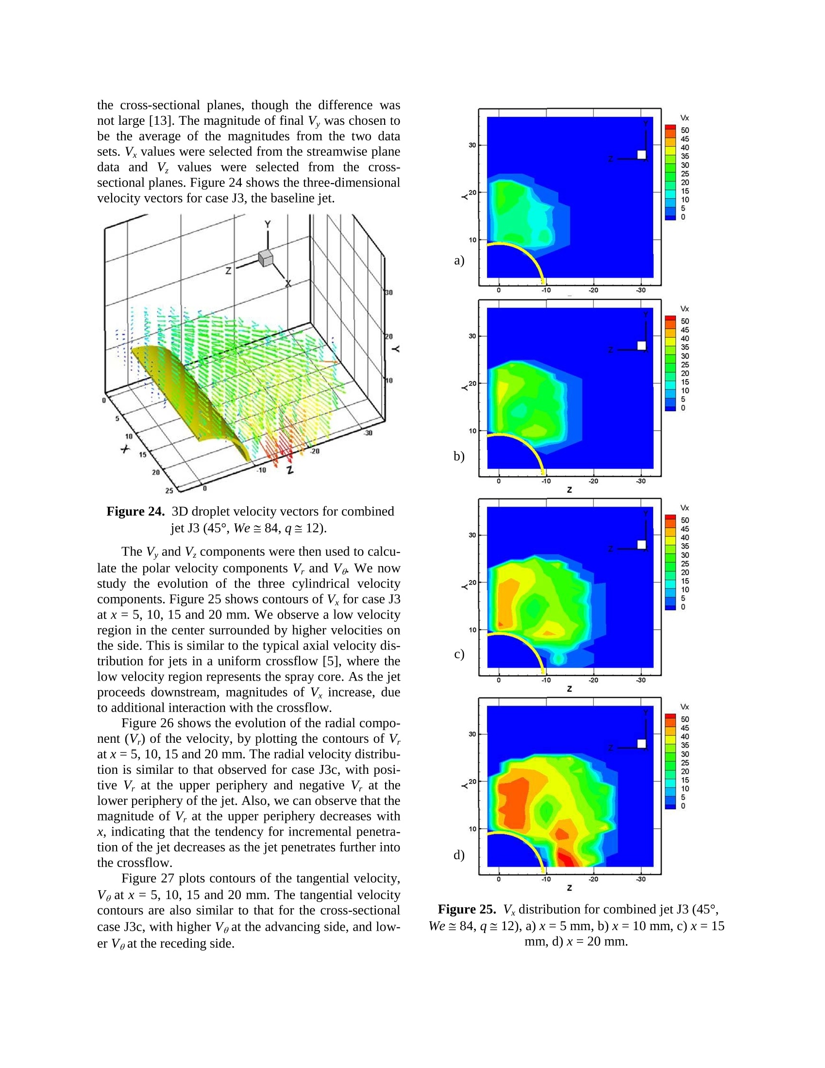
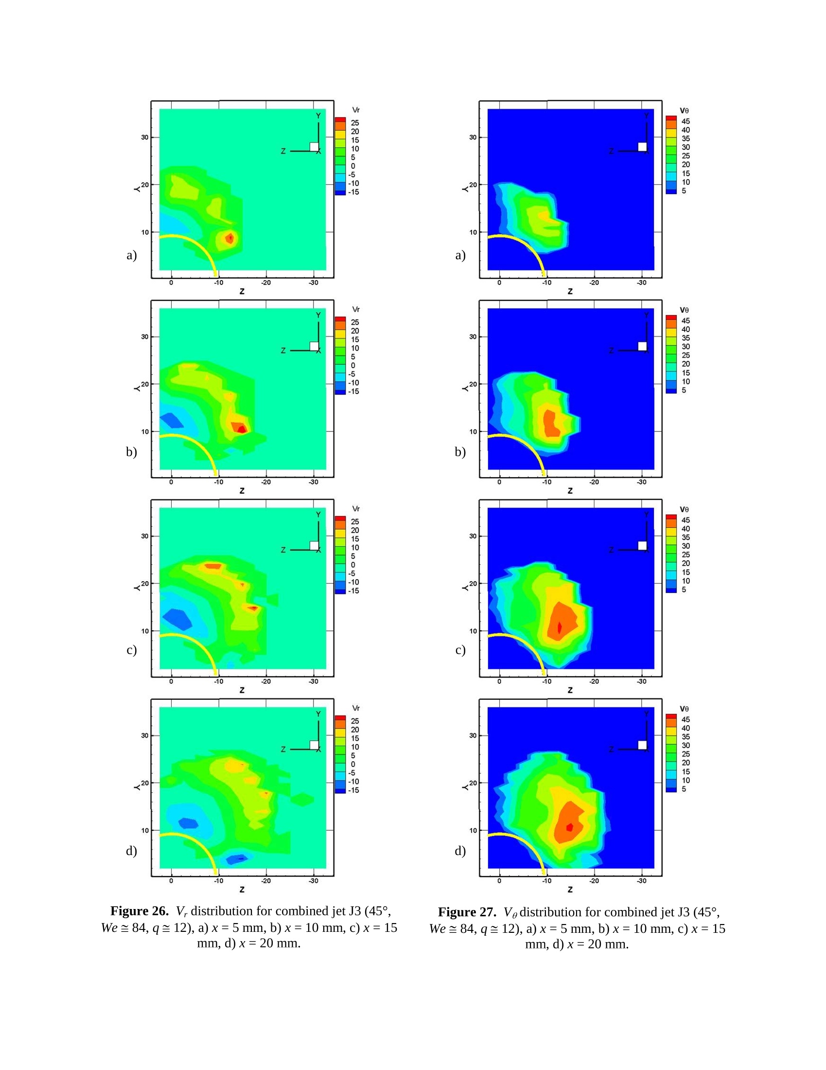
ILASS Americas， 22"d Annual Conference on Liquid Atomization and Spray Systems， Cincinnati， OH， May 2010 Three-Dimensional Penetration and Velocity Distribution of Liquid Jets Injected Trans-versely into a Swirling Crossflow Samir B Tambe and San-Mou Jeng Department of Aerospace Engineering and Engineering Mechanics University of Cincinnati Cincinnati， OH 45221 USA Abstract An experimental study has been conducted to study the effect ofa swirling crossflow on transversely injected liquidjets. In-house designed axial swirlers with vane exit angles of 30°，45° and 60°were used to generate the swirlingcrossflow. Laser Doppler Velocimetry (LDV) results indicate that the axial (U.) and the tangential (Ua) componentsof the crossflow velocity decrease with increasing radial distance from the center. Also， flow angle (y) of thecrossflow is lesser than the swirler vane exit angle indicating that the swirlers did not impart sufficient tangentialmomentum for the flow to be parallel to the vanes at swirler exit. The deficit in flow angle increased with swirlerangle. Water jets were injected from a 0.5 mm diameter orifice located on a cylindrical centerbody that protrudedthrough the hub of the swirler. Particle Image Velocimetry (PIV) was used to study the behavior of the jets. PIVmeasurements were conducted in multiple cross-sectional and streamwise planes. Mie-Scattering images were col-lated to create three-dimensional representation of the jet plume， which was used to study penetration. In cylindricalcoordinate system， the penetration can be described in terms of radial and “circumferential”penetration， where cir-cumferential penetration is defined as the difference in the circumferential displacement of the jet and the crossflowover the same streamwise displacement. Increasing the momentum flux ratio (q) resulted in a higher radial penetra-tion. Increasing the swirl angle reduced radial penetration and increased circumferential penetration. PIV results ofthe cross-sectional and streamwise planes each yielded two velocity components which were merged to obtain three-dimensional droplet velocity distribution. The three-dimensional velocity distribution yielded further insight into theevolution of the jet plume. ( C orresponding author ) Introduction The transversely injected liquid jet in crossflow hasnumerous applications including fuel injection [1]，thrust vector control of rockets [2]， and lubrication ofthe bearing chamber [3]. The injection of a liquid fueljet into crossflow is also one of several possible con-cepts of a premix module for lean， premixed， prevapo-rized (LPP) combustion for aviation gas turbines. Thedemands for higher efficiency of power production andsmaller engines lead to an increase in the operatingtemperatures and pressures. This leads to increase in theproduction of effluents like oxides of nitrogen (NOx)since NOx formation rates increase with temperature[4]. With the increasingly stricter ICAO regulations onengine emissions， there is a strong emphasis on the de-velopment of low-emission combustion techniques.One technique is the LPP combustion， where lean， ho-mogeneous fuel-air mixture is created just upstream ofthe combustor inlet. Thepresence of excessairthroughout the primary zone ensures that the combus-tion temperature is low enough to suppress NOx forma-tion. The LPP model requires a premix duct where fueland air are mixed together. To achieve good homoge-neous mixture and to avoid coking， fine atomizationand careful fuel placement are needed. Liquid jet incrossflow has characteristics of rapid atomization andcontrollable penetration [1]， which make it a goodchoice for LPP fuel injection. Jet-in-crossflow is a fundamental flow field andhas been the subject of numerous experimental as wellas computational studies. Tambe [5] and Elshamy [6]have conducted detailed literature reviews of the workdone in this area. However， most of the studies featureuniform crossflows， i.e. where crossflow velocity doesnot change in the transverse direction. Only a few stu-dies have utilized crossflows with steady-state non-uniform velocity profiles. Becker and Hassa [7， 8] in-jected liquid jets into a counter-swirling double-annularcrossflow and studied the effect of momentum fluxratio and air pressure on the jet behavior. Gong et al [9]published a preliminary report on studies conducted forthe Lean Direct Wall Injection (LDWI) concept， wherethey injected liquid jets into a swirling flow at differentinjection angles. The authors previously conducted astudy where jets were injected transversely into acrossflow laden with a shear layer [10， 11]. The shearlayer was generated by creating a slip plane betweentwo co-flowing airstreams， creating a quasi-linear ve-locity gradient in the transverse direction. The strengthof the shear layer and the sense of the velocity gradienthad a significant impact on the jet penetration and thepost-breakup spray. The objective of the present work is to study thebehavior of a liquid jet injected transversely into aswirling crossflow. The effect of swirl strength， in addi-tion to typical jet parameters， on the jet penetration and the droplet velocity distribution was investigated. Theswirl strength was varied by using three different axialswirlers with different vane exit angles. Experimentaltechniques used include Laser Doppler Velocimetry(LDV) and 2-D Particle image Velocimetry(PIV). Thestudy was divided into a thorough investigation of thecrossflow before looking at jets and the impact of thiscrossflow on their behavior. A part of this study [12]was reported previously. This paper serves to extendthe findings from the previous paper. In this study， LDV was used to study the crossflowto avoid the signal-to-noise issues experienced duringPIV measurements [12].PIV measurements were con-ducted on the jet at multiple cross-sectional as well asstreamwise planes. The Mie-Scattering images from thecross-sectional planes led to an improved penetrationprediction. Also， as each plane yielded two componentsof droplet velocity， the results were combined to createthree-dimensional droplet velocity distribution. b) Figure 1. Test Chamber， a) Model， b) Test Chamber. Experimental Setup Test Chamber The test chamber has a square cross-section withan internal dimension of 7.62 cm (3”) and is 30.48 cm(12”) long. The walls of the test chamber are con-structed of 3.175 mm (1/8”) thick acrylic material formaximum optical access. The walls are mounted onaluminum corner struts， which also provide a chamferto suppress corner recirculation zones. Figure la shows a model of the test chamber as-sembly and also indicates the coordinate frame of refer-ence used for all analysis. Figure 1b shows the testchamber. The origin of the coordinate frame is locatedon the axis of the centerbody at the streamwise locationof the center of the jet orifice. X-axis is aligned with the streamwise direction， Y-axis points vertically upwardsand Z-axis points to the left as viewed from down-stream. The test chamber assembly is mounted onto theHorizontal Rig， which is one of the experimental rigsavailable at the Combustion Diagnostics Research La-boratory at the University of Cincinnati’s Center HillFacility. The Horizontal Rig is a long pipe 15.24 cm(6”) in diameter， and is equipped with a 72 kW inlineair heater (not used for this study). A computer con-trolled 3-axis Lintech traverse is provided for precisepositioning of diagnostic equipment. Air is providedfrom a Kaesar variable speed rotary compressor capableof maximum flow rate of 0.907 kg/s (2 lb/s) at a pres-sure of 7.9 bars (100 psig)， connected to a dryer andtanks. A network of 10.16 cm (4”) and 5.08 cm (2”)diameter pipes connects the air tanks to the HorizontalRig. Air flow rate is metered by a Micro MotionCMF300 coriolis flowmeter and controlled by a stan-dard gate valve. Jet injection is carried out through a centerbody，which protrudes from the swirler hub and extendsthrough the length of the test chamber. The centerbodyis a 1.91 cm (3/4”) outer diameter stainless steel tubewith wall thickness of 1.65 mm (0.065”). Thus the ra-dius of the centerbody， rcb =0.96 cm. A water jet isinjected from a 0.5 mm orifice located 2.54 cm (1”)downstream of the swirler exit. The centerbody isaligned so that the jet orifice is centered on the Y-axis.Thus the coordinates of the center of the orifice are (0，rcb，0). The injected liquid is water， and is housed in awater tank. A nitrogen cylinder is used to pressurize thewater tank， in order to drive the flow， as well as main-tain a constant flow rate. The water flow rate is meas-ured by a Micro Motion CMF010 coriolis flowmeter. AParker metering valve is used for precise control of thewater flow rate. Figure 2 shows a schematic of the ex-perimental setup. Swirlers The axial swirlers used for the study were designedin-house and were fabricated by Rapid PrototypingSLA technology. The swirlers feature a hub diameter of2.22 cm (0.875”) and a tip diameter of 7.62 cm (3”). A1.91 cm (3/4”) diameter hole is provided in the hub toaccommodate the centerbody. Three different swirlerswere used， with vane exit angles of 30°， 45° and 60°. The swirlers have a streamwise depth of 2.54 cm(1”) with 12 vanes each for the 45° and 60° swirlers. Toachieve reasonable solidity， the number of vanes wasincreased to 16 for the 30° swirler. The vanes wereradial， and designed to provide a smooth transition fromaxial direction to the vane exit angle. Figure 3 shows acutout of the 45° swirler design model as well as a fa-bricated swirler. All swirlers induce a swirl in theclockwise direction， as viewed from downstream. Figure 2. Schematic of Experimental Setup. a) b) Figure 3. 45° Axial Swirler， a) Model， b) Swirler. Measurement Techniques LDV measurements were conducted to characterizethe crossflow. The equipment used for LDV measure-ments is the PDI-200 from Artium Inc. The PDI-200series consists of a transmitter， a receiver， a powersupply for the transmitter， and signal processing sys-tem. The special feature of the PDI-200 system is thatthe lasers are housed within the transmitter itself， sothat there is no need for fiber optic systems， and therelated alignment issues. The lasers used are DiodePumped Solid State (DPSS) lasers， which do not re-quire active cooling， and hence can be housed within acompact transmitter body. The PDI system was operat-ed in LDV mode with forward scatter at an angle of15°. The crossflow was seeded with olive oil droplets toenable measurement. For each test case， measurementswere conducted in a cross-sectional plane 2.54 cm (1”)downstream of the jet injection (x=2.54 cm). Figure 4shows a schematic of the setup for the LDV measure-ments. 2-D PIV was used for jet flow measurements. ThePIV system is a LaVision commercial PIV system. ANewWave Solo PIV， double-pulsed Nd：YAG laseremits laser pulses at a wavelength of 532 nm with amaximum energy of 120 mJ/pulse. A LaVision ImageIntense， double frame - double exposure CCD cameraacquires images at the rate of 5 image pairs per second.A bandpass filter at 532 ±3 nm is used to restrict the Case no Swirler We mef(kg/s) U(m/s) U(m/s) U (m/s) (deg) w=f(r) Pef20 (deg)， r=20mm， Ax=20 mm C1 30 32.55 0.226 54.28 31.35 62.69 30 w=0.9721r+8.6，R=0.9883 30.5 C2 (base) 45 33.91 0.222 50.67 38.95 63.91 37.5 w=1.2054r+9.7，R=0.5018 38.4 C3 60 25.98 0.175 40.37 39.13 56.22 44.1 w=1.538r+11，R=0.9437 51.2 C4 60 49.35 0.24 55.41 54.12 77.46 44.3 w=1.4937·r+12.2，R^=0.9234 51.8 Table 1. Test conditions and relevant parameters for crossflow studies. light absorbed to the laser wavelength. For more detailson the PIV system， please refer to Elshamy [6]. Figure 4. Schematic of LDV Setup. Figure 5. Schematic of PIV Setup. PIV/ measurements were conductedd incross-sectional planes， i.e. parallel to the YZ plane (x=con-stant). Measurement was conducted over a range ofx=0：25 mm， with a spacing of 2.5 mm between measure-ment planes. Additionally， a few of the cases were re-peated with measurements in streamwise planes， i.e.parallel to the XY plane (z= constant). The measureddomain was z = 0：-30 with the planes separated by 2.5mm. The centerbody was coated with a fluorescent paintto reduce noise due to reflection. The paint convertsabout 30% of the green laser light into red fluorescentlight， which gets blocked by the bandpass filter on thecamera. Figure 5 shows the schematic of the PIV formeasurement in the x=constant planes. Test conditions The 45°swirler was considered as the base swirler.Table 1 lists the test conditions used for crossflow stu-dies. Table 2 lists the test conditions for jet measure-ments for cross-sectional (x=constant) as well asstreamwise (z = constant) planes. The test cases for jetswere designed so that the streamwise planes would re-peat the test conditions for the cross-sectional planes.Thus cross-sectional and streamwise measurements forcase J3 are represented by cases J3c and J3s respective-ly. The base cases for the crossflow and the jet are casesC2 and J3. The Weber number (We) and the momentumflux ratio (q) described in the test conditions were cal-culated based on total crossflow velocity， which wasobtained from LDV results as explained in the resultssection. For water， a density of 996 kg/m’ and a surfacetension of0.0072 N/m have been assumed. Results and Discussion Note on Polar domain Since the nature of the crossflow is axisymmetric，it was considered more useful to analyze the flow in acylindrical domain. However， since all measurementsare conducted in cartesian planes， the measured do-mains need to be transformed. The process occurs in a x= constant plane， where (， z) coordinates are trans-formed into (r，) coordinates (Figure 6). A new polargrid was created， and properties at the new grid points...were obtained by interpolation. The polar grid， alongwith the X-axis， completes the cylindrical domain. Also，since the jet orifice is located on the 12 o’clock positionon the centerbody， the circumferential coordinate isoriented such that 0=0°at the positive Y-axis and in-creases in the clockwise direction， as seen from down-stream. Case No Swirler We q mef(kg/s) U.(m/s) U(m/s) U (m/s) mj (kg/min) V (m/s) MeasurementPlane 'p，x=20mm 0p，20，(deg)，x=20mm J1c 30 106.16 9.42 0.401 99.59 57.5 114.99 0.141 12.02 cross-sectional 18.3 4 J2c 45 42.27 12.05 0.245 57.14 43.92 72.07 0.101 8.58 cross-sectional 16.3 6.5 J3c (base) 45 83.72 12.02 0.345 80.42 61.82 101.41 0.142 12.06 cross-sectional 19.3 6.5 J4c 45 83.72 24.01 0.345 80.42 61.82 101.43 0.2 17.05 cross-sectional 21.3 7.5 J5c 60 51.66 19.6 0.243 57.38 56.06 80.22 0.142 12.1 cross-sectional 20.3 9.3 J6c 30 106.16 18.94 0.401 99.59 57.5 114.99 0.2 17.05 cross-sectional 22.8 5 J7c 60 51.56 39.16 0.243 57.28 55.95 80.07 0.201 17.09 cross-sectional 26.3 11.3 J1s 30 106.35 9.4 0.401 99.77 57.6 115.21 0.141 12.02 streamwise - - J2s 45 42.76 11.91 0.245 57.8 44.43 72.9 0.101 8.58 streamwise J3s (base) 45 84.69 11.96 0.345 81.35 62.53 102.61 0.142 12.1 streamwise - - J4s 45 84.69 23.84 0.345 81.35 62.53 102.61 0.2 17.09 streamwise - - J5s 60 52.08 19.44 0.245 57.31 55.99 80.12 0.142 12.1 streamwise - Figure 6. Transformation to Polar coordinates. Now， if the data is contained within a cross-sectional plane， the properties at the locations of thenew domain can be obtained by interpolation withoutany significant loss of information. However， for mea-surements in streamwise planes， a slice of the dataset atx= constant contains data only at discrete locations. Inthis case， carrying out interpolations for the new polar grid may omit significant information due to the in-completeness of data. In the previous report [12]， inten-sity (Mie-Scattering) measurements along streamwiseplanes were converted into polar domain for penetrationstudies. While this yielded relatively good results in theradial direction， the circumferential coordinates clearlyexhibited a lack of good resolution due to interpolationbetween measurement planes. To avoid this issue in thisstudy， the conversion to cylindrical domain was con-ducted only for measurements in cross-sectional planes. Crossflow Structure It is important to characterize the crossflow in or-der to study its effects on the jets. This was achieved byconducting LDV measurements at the x = 25.4 mm -30 -20 -10 0 10 20 a) 巧如们505和佰加 30 0 -20 -30 Figure 7. LDV results， Crossflow case C2 (45°， We=33.91)； a) Measurement grid， b) U. contours， c) U， contours. plane. Figure 7a shows the measurement grid. Figures7b and 7c show the contours of the streamwise (U.) andthe vertical (U，) components of the velocity，respective-ly， for case C2， the base crossflow. Case C2 features the45° swirler with We =33.91. The centerbody isrepresented by the black circle in Figure 7. We observethat U.is high near the centerbody， while the absolutemagnitude of U， is low near the Y-axis， but high nearthe Z-axis. U， is negative in the right half plane due tothe clockwise sense of rotation imparted by the swirler. A polar grid was created， and the U， and U， com-ponents were mapped to the new grid by interpolation.Now， since the flow issuing from the swirler is axi-symmetric， we can predict the z-component of thecrossflow velocity， U， by rotating the domain by 90°.In this process， U， at a location (r， ) gets mapped to Uat (r， 0± 90°). Due to gaps in the LDV measurement，the circumferential extent of the region where both U，and U， are known is limited to 30°≤0≤60°. The totalvelocity， U was obtained as a vector sum of the threevelocity components. Using trigonometric relations， U，and U， were transformed into polar velocity compo-nents， U， and Up. A detailed description of this proce-dure is given in Tambe [13]. Figure 8 plots the variation of the total velocity，and its cylindrical components， with r for case C2.From Figure 8 we observe that both U， and U， decreasemonotonically with r while U initially increases with rthough it starts decreasing at high r. The total crossflowvelocity， U decreases monotonically with increasing r.The magnitude of U， was observed to be very smallcompared to the other components， and will be neg-lected from further discussion. Figure 8. Total velocity andcylindrical velocity com-ponents for crossflow case C2 (45°， We=33.91). Figure 9 plots U. and U for cases C1-C4. The cal-culated We for cases C1 (30°)， C2 (45°)， C3 (60°) andC4 (60°) were 33， 34， 26 and 49 respectively. FromFigure 9， we observe that as swirl angle increases， Ue increases while U. decreases. As swirl angle increases，highertangential mmomentum is impartedto thecrossflow causing U to increase. Now since We forcases C1 and C2 are almost equal，C2 will have smallerU in order to maintain the same total velocity. We notethat U for case C3 is slightly lower than that for caseC2， though this occurs mainly because We of case C3 isless than that for case C2. Comparing the velocities forcases C3 and C4， we observe that increasing We leadsto increase in both U， and Ue. Figure 9. U. and Udistributions for crossflow cases. From the total and axial velocities， we can calcu-late the local flow angle， w， from equation 1. The flowangle is the angle made by the velocity vector with thestreamwise direction (positive X-axis). Figure 10 plotsthe flow angles for cases C1- C4. For each swirler， theflow angle increases with r even though both U. and Uedecrease. Linear fits were obtained to describe the vari-ation of y with r and have been included in Table 1.Mean y were determined based on mean U， and Ug andare also listed in Table 1. We observe that the mean wfor the 30°， 45° and 60°swirlers are 30°， 37.5° and44.3° respectively. Thus， only the 30° swirler generatesenough flow turn from the crossflow. Thus， at the exit Figure 10. Flow angles (y) for crossflow cases. of the swirler， the flow velocity is not tangent to thevanes， indicating that the 45° and 60° swirlers could notimpart sufficient flow turn to the crossflow. From Table 1 and Figure 10， we observe that Wedoes not have any effect on the flow angle， w (CasesC3， C4). The only change is an increase in the magni-tudes of the velocity components. Another parameter of importance is the circumfe-rential displacement (d)， which is the shift in the cir-cumferential () position of a particle for a given dis-placement in x. We have observed that the flow angle，y depends upon r. Then at any radius， o for a given ▲xwill also depend upon r and can be calculated fromequation 2. The magnitudes of Pefx for cases C1-C4 atmeanr=20 mm andAx =20 mm have been calculatedand are listed in Table 1. Thus for case C2， a particlelocated at r= 20 mm undergoes a circumferential dis-placement of 38.4° as it moves 20 mm downstream. Jet Measurements The difficulty with studying jets in a swirling flowis that we do not know the trajectory of the jet. The pathfollowed by the jet is curved， so that its cross-section isno longer parallel to the YZ plane. This was sought tobe remedied by taking PIV measurements at severalparallel planes and combining them together to create a3-D measurement domain where we can re-create thejet plume. In the previous work [12]， this was sought byconducting measurements in streamwise planes. How-ever， as was shown earlier， when converting to cylin-drical domain， interpolation occurs between measure-ment planes where no data is available. As a result， weare more likely to miss features of the jet that werepresent outside the measurement planes. Figure 11. Mie-Scattering images for cross-sectionaljet case J3c (45°， We=83.72，q=12.02). To alleviate this problem， PIV measurements wereconducted in cross-sectional (x= constant) planes.Then， all interpolations for the conversion to polarcoordinates occur within the measurement plane， so thatthe risk of missing out on details of the jet is mini-mized. Additional tests were conducted with measure-ments in streamwise (z= constant) planes to match thetest conditions of the cross-sectional planes cases.Allthese test conditions have been listed in Table 2. Recreation of the Jet Plume Case J3， with We=84， q= 12 for the 45° swirlerwas considered as the base jet case. The correspondingcase number for cross-sectional PIV is case J3c. Weillustrate here the procedure for recreating the jet plumeand obtaining the penetration for the jet. From PIV results， we obtain an averaged Mie-Scattering image for each x=constant plane (Figure11). These can also be obtained as Tecplot data files，which are essentially intensity maps， i.e. they containcoordinate information with intensity values at thesecoordinates. A Matlab program was created to add thethird (x) coordinate and combine all planes into a singledata file. Additionally， the Mie-Scattering intensities ineach measurement plane were normalized by the max-imum intensity in that plane to provide comparableintensities across measured planes. Tecplot then rendersthis file as a 3-D plot of intensities， and can then beused to plot out the isosurfaces of the jet. An isosurfaceis the collection of all locations which have the sameintensity value. The jet plume is thus represented byisosurfaces of the normalized Mie-Scattering intensity. Figure 12. 3D Jet plume for case J3c (45°， We=83.72，q=12.02). Jet Plume Figure 12 shows the isosurfaces for the base jet，case J3c. Figures 13a， b， c show the projected views ofthe spray plume onto the XY， XZ， and YZ planes respec-tively. The edges of the cylindrical domain and the lo-cation of the centerbody are also illustrated in Figures12 and 13. While the streamwise (x) momentum of thecrossflow causes the jet to bend in the streamwise di-rection， the tangential () momentum also induces amotion in the circumferential (e) direction. Thus thetrajectory of the jet is curved， forming an angle to thestreamwise direction similar to the flow angle of thecrossflow. This also means that the jet cross-section isat an angle to the measurement plane， causing its widthto appear smaller. As a result， the shape of the jet plumeappears to be elliptical (Figures 11， 12， 13c). Z Figure 13. Projected views of spray plume for caseJ3c (45°，We=83.72，q=12.02)，a) XYplane， b) XZplane， c) YZ plane. Detecting Jet Boundary In order to detect the jet boundary， a threshold wasapplied to the Mie-Scattering images. The thresholdwas set at 10% of the maximum intensity of the plane，with all locations with higher intensity being considered a part of the jet. A boundary detection algorithm wasthen used to trace the boundary of the jet plume at eachmeasurement plane. From each boundary trace， 4 pointswere manually selected， marking the radial and circum-ferential extremities of the jet. The radial edges are theupper and lower edges of the jet while the circumferen-tial edge on the advancing side is called the right edgeand the other side is called the left edge， based on theappearance as viewed from downstream. Now， sincethe trajectory is three-dimensional， each edge locationhas r as well as 0 coordinates. Both need to be takeninto account while describing jet penetration. Jet Penetration We saw above that there are two dimensions to thejet trajectory， due to the presence of the radial and thecircumferential coordinates of the edge. To understand how this affects the jet， we first con-sider the case of a regular jet in crossflow， i.e. a jet in-jected transversely into a uniform crossflow. The aero-dynamic forces exerted by the crossflow cause the jet tobend and it starts to move along the streamwise direc-tion， so that the jet trajectory is aligned with the direc-tion of the crossflow velocity. Note that this would stillbe valid if the streamwise direction (direction ofcrossflow velocity) was not aligned to any particularcoordinate axis， i.e. if it had non-zero componentsalong the X and Z axes. The jet trajectory would still beparallel to the direction of the crossflow velocity. Now let us consider a simplified version of ourcrossflow in R-O domain， assuming that U， and Udonot vary with r. Due to axisymmetry， U. and Udo notchange with 0. Then， within this domain， the crossflowis similar to the previous example， and the jet trajectorywould align with the direction of the crossflow velocity，i.e. it will have a flow angle equal to that of thecrossflow. In this case， the jet trajectory has only onedimension， the radial height of the jet periphery， whichcan be referred to as the radial penetration(r)). Thecircumferential coordinate， even though it exists， doesnot add any extra information about jet penetration andcan be neglected under these conditions. However， in the physical domain， a streamline ofthe crossflow is not a straight line， but follows a helicalpath. Thus the crossflow is subject to centripetal accele-ration， which causes the streamline to curve in on itself，creating the helical nature of the streamline. Now， inaddition to aerodynamic forces， tangent to the crossflowstreamlines， the momentum of the jet also has to coun-ter centripetal forces， directed radially inward. This hastwo effects. The first effect is an increase in radial pe-netration， akin to the effect of“centrifugal” forces. Se-condly， this would also cause the jet trajectory to have alower average flow angle as compared to the crossflow.This means that the circumferential displacement (0) ofthe jet over a given streamwise displacement would be lower than that of the crossflow. This difference in cir-cumferential displacement is referred to as the circum-ferential penetration(0，). Then， radial penetration (r，) at any x-location is de-fined as the radial distance of the outer jet peripheryfrom the surface of the centerbody. It is standard prac-tice to scale the penetration by the jet diameter， d [1，5，6] to allow comparison across different datasets anddifferent studies. Then r， can be calculated as shown inequation 3. The circumferential penetration (Pp，x) at any x-location is defined as the difference in the total circum-ferential displacements of the crossflow (中er) and the jet(g) over the streamwise range of x=0 to the said x-location. Po.x can be obtained from equation 4， whereofor both jet and crossflow at x=0 are assumed to be 0. Table 2 also lists r， and p，x for all the cross-sectional jet cases at x = 40d (20 mm). For calculatingp， Ver was obtained based on yat r=20 mm. Figure 14. Radial penetration (r) for case J3c (45°，We=83.72，q=12.02). Figure 14 shows radial penetration for the baselinejet， case J3c， and compares it to the penetration of anequivalent jet-in-uniform-crossflow (q = 12)， obtainedfrom the penetration correlation of Tambe [5]. We ob-serve that in the near-field， the penetrations of both jetsare similar. However as the jets move further down-stream， the jet-in-swirling-crossflow continues to pene-trate much higher as compared to the one from the cor-relation. As explained earlier， the jet in the current caseexperiences centrifugal acceleration， which might ac-count for high radial penetration. Additionally， fromFigure 9， we see that the crossflow velocity， U decreas-es with r. This creates a situation similar to the case in Tambe et al [10]， where crossflow velocity decreaseswith height. As the jet penetration increases， the aero-dynamic force exerted by the crossflow decreases， al-lowing relatively higher incremental penetration ascompared to a case with a constant crossflow velocity. Figure 15. Circumferential progress of the jet， caseJ3c (45°， We=83.72，q=12.02). We next consider the circumferential penetration ofthe jet. Figure 15 plots the circumferential (O) coordi-nates of the top， left and right edges for the baseline jetcase J3c. We observe that the top periphery is slightlycloser to the left periphery as compared to the right； thisoccurs since the jet plane is at an angle to the measurement plane. Figure 15 also plots the circumferentialprogress of a particle in the crossflow located at aheight ofr=20 mm. We observe that the circumferen-tial displacement of the jet is indeed less than that of thecrossflow， supporting the concept of circumferentialpenetration. Figure 16. Effect of swirl angle onr. We next study the effect of jet and crossflow para-meters on jet penetration. Though not illustrated here， itwas found that q affects onlyrp， while We had no sig-nificant effect on penetration (Table 2). Here we con-sider the effect of swirl strength on radial penetration.Figure 16 plots the radial penetrations of cases J6c(30°)， J4c (45°) and J5c (60°)， along with the uniform crossflow penetration correlations for the correspondingq values. We observe that the radial penetrations for all3 cases are very close to the predicted penetrations fromthe correlation in the near region. However， beyond theinitial region， the penetration for case J6c (30°) seemsto be the highest， and is nearly equal to that for case J4c(45°)， even though q for J4c is higher. An explanationfor this could be that as swirler angle increases， moretangential momentum is imparted to the jet， causingreduced resistance in the radial direction， leading tolower penetration. From Figure 17， which plots the cir-cumferential displacements for the same cases， we ob-serve that the circumferential displacements do increasewith swirl angle， thus supporting the previous claim.Figure 17 also plots the circumferential displacementsof the crossflow. We observe that even though the cir-cumferential displacement of the jets increase， the cir-cumferential penetrations also increase with an increasein the swirl angle. Figure 17. Effect of swirl angle on circumferentialprogress of jets. Jet Velocities For droplet velocities of the jet， we first considerthe results from PIV measurements in the cross-sectional (x= constant) planes. Test conditions havebeen listed in Table 2. We select the baseline jet， caseJ3c for detailed analysis. Figure 18 shows PIV resultsfor case J3c at two measurement planes， x=5， 10 mm.The results from the different planes were collated in amanner similar to the Mie-Scattering images. Addition-ally， the measurement domain was converted into cy-lindrical domain， and the cartesian velocity components(V，V)， were converted to polar velocities (V，Va). Figure 19 shows the velocity vectors for case J3c atstreamwise locations of 5， 10， 15 and 20 mm down-stream of the nozzle. We can clearly observe the spreadof the spray plume as the jet moves downstream. Oneof the surprising features of the jet is that most of thevelocity seems to be directed in the tangential direction，even though we know that the jet grows in the radial as well as the tangential direction. To understand thismore clearly， we take a closer look at the radial (V，) andthe tangential (Ve) velocity components for case J3c.Figures 20 and 21 plot V， and Vo， respectively，at thesame locations as Figure 19. From Figure 20， we ob-serve a zone of positive V，. at the upper and upper-rightportion of the plume， and a negative V， region towardsthe bottom and bottom left. This accounts for the spreadof the jet in the radial direction. From Figure 21， weobserve high V in the right half of the jet plume， whilethe left half has low， positive Ve. This shows that theentire jet plume experiences positive circumferentialdisplacement， and that it is also expanding in the tan-gential direction. We note here that the highest Ve wasapproximately 63 m/s， while the average tangentialvelocity of the crossflow， Ue was 62 m/s (Table 2， caseC2). Thus， even though the jet plume moves circumfe-rentially， the rate of circumferential displacement islower than that of the crossflow， thereby reinforcing theconcept of circumferential penetration. Figure 18. PIV results for cross-sectional planes， jetcase J3c (45°， We=83.72，q=12.02). Next， we consider the results from PIV measure-ments in the streamwise (z= constant) planes. The testconditions have been listed in Table 2. The test condi-tions were designed to be equivalent to the cases forcross-sectional measurement， and hence have similarcase numbers， with the last letterc’being replaced by‘s'to denote streamwise plane measurements. Thus thebaseline jet for streamwise plane PIV is case J3s. Themeasurement domain for streamwise planes is the topright quarter of the test chamber， i.e.z<0，y>0 (Figurela). Figure 22 shows the PIV results for case J4s at twoplanes located at z=-5，-10 mm. The velocity components in the streamwise plane(V，V) can be collated in a manner similar to the cross-sectional components to form a three-dimensional mea-surement domain. Figure 23 shows the velocity vectordistribution at z=-5，-10 mm along with the location ofthe centerbody， which is visible at z=-5 mm. However，since V is not known， we cannot obtain polar velocitycomponents for this data. V 65 Z 60 30 -55 50 40 35 30 <20 -25- 20 15 10 5 10 a) 10 -10 -20 -30 Z V 65 Z 30 60 55 50 45 40 35 <20 30 20 15 10 5 10 b) 10 -10 -20 -30 Z Z Figure 19. Droplet velocity distribution for case J3c(45°，We=83.72，q=12.02)，a)x=5 mm， b)x=10mm， c)x=15 mm，d)x=20 mm. Figure 20. V. distribution for case J3c (45°， We=83.72，q=12.02)，a)x=5 mm，b)x=10 mm， c)x=15mm， d)x=20 mm. Z Figure 21. Vdistribution for case J3c (45°， We=83.72， q=12.02)，a)x=5mm，b)x=10 mm， c)x=15mm，d)x=20 mm. Three-Dimensional Velocity Distribution Since the test conditions for the measurements forthe cross-sectional and streamwise planes were equiva-lent， it allows us to merge the two datasets. A 3D carte-sian grid was defined， ensuring that it was coarser thanthe two measured domains to ensure smoother interpo-lation of data. Both datasets have a vertical velocitycomponent， .. Upon comparing ， for the two sets ofdata， it was observed that the magnitude of V， for thestreamwise planes was consistently higher than that for Figure 22. PIV results for streamwise planes， jet caseJ3s (45°，We=84.69，q=11.96). Figure 23. Droplet velocity distribution for case J3s(45°， We=84.69，q=11.96)，a) z=-5 mm， b)z=-10mm. the cross-sectional planes， though the difference wasnot large [13]. The magnitude of final V，was chosen tobe the average of the magnitudes from the two datasets.V. values were selected from the streamwise planedata and V. values were selected from the cross-sectional planes. Figure 24 shows the three-dimensionalvelocity vectors for case J3， the baseline jet. Figure 24. 3D droplet velocity vectors for combinedjet J3 (45°， We= 84，q=12). The V， and V， components were then used to calcu-late the polar velocity components V， and V. We nowstudy the evolution of the three cylindrical velocitycomponents. Figure 25 shows contours of V.for case J3at x= 5， 10， 15 and 20 mm. We observe a low velocityregion in the center surrounded by higher velocities onthe side. This is similar to the typical axial velocity dis-tribution for jets in a uniform crossflow [5]， where thelow velocity region represents the spray core. As the jetproceeds downstream， magnitudes of V. increase， dueto additional interaction with the crossflow. Figure 26 shows the evolution of the radial compo-nent (V，) of the velocity， by plotting the contours of V，at x= 5， 10， 15 and 20 mm. The radial velocity distribu-tion is similar to that observed for case J3c， with posi-tive V， at the upper periphery and negative V，. at thelower periphery of the jet. Also， we can observe that themagnitude of V， at the upper periphery decreases withx， indicating that the tendency for incremental penetra-tion of the jet decreases as the jet penetrates further intothe crossflow. Figure 27 plots contours of the tangential velocity，Ve at x= 5， 10， 15 and 20 mm. The tangential velocitycontours are also similar to that for the cross-sectionalcase J3c， with higher Ve at the advancing side， and low-er Ve at the receding side. Figure 25. V.distribution for combined jet J3 (45°， We84，q= 12)，a)x=5 mm，b)x=10 mm，c)x=15mm，d)x=20 mm. 33xx33x31x s3xux33313x1 Conclusions We have studied liquid jets injected into a swirlingcrossflow. The crossflow was non-recirculating， withboth axial and tangential velocities decreasing withradius. We studied the jet penetration and observed thatthe penetration needs to be separated into radial andcircumferential penetration to completely describe thejet trajectory. PIV velocity measurements were con-ducted in cross-sectional as well as streamwise planes，and the velocities were combined to generate a 3-Dvelocity distribution. Nomenclature d iet diameter m mass flow rate momentum flux ratio r radial coordinate x streamwise coordinate vertical coordinate zlateral coordinateUXYZ radial axis crossflow velocity droplet velocity streamwise axis vertical axis lateral axis We aerodynamic weber number circumferential displacement circumferential coordinate flow angle circumferential axis Subscripts cfcrossflow jjetrradial component x streamwise component vertical componentz lateral component circumferential (tangential) component ( References ) 1. Becker， J.， and Hassa， C.， Atomization and Sprays11：49-67 (2002) 2. Chen， T.H.， et. al.，31" Aerospace Sciences Meetingand Exhibit， Reno， NV 1993 3. Birouk， M.， Azzopardi， B. J.， and Stabler， T.， Par-ticle and Particle Systems Characterization 20：283-289 (2003) 4.Lefebvre. A.W.， Gas Turbinee (Combustion.McGraw-Hill， 1983， Ch 9. 5.TTambe， S.B.， Liquid Jets in Subsonic Crossflow，”MS Thesis， Department of Aerospace Engineeringand Engineering Mechanics， University of Cincin-nati， Cincinnati OH (2004) 6. IElshamy， O.M.，，“Experimental Investigations ofSteady and Dynamic Behavior of Transverse LiquidJets，” PhD Dissertation， Department of AerospaceEngineering and Engineering Mechanics， Universityof Cincinnati， Cincinnati OH (2007) 7. Becker， J.， and Hassa， C.， Journal of Engineeringfor Gas Turbines and Power， 125：901-908 8. Becker， J.， Heitz， D.， and Hassa， C.， Atomizationand Sprays， 14：15-35 (2004) 9.(Gong et. al.， Journal of Propulsion and Power，22：209-210 (2006) 10.Tambe， S.B.，Elshamy， O.M.， and Jeng， S.-M.， 45"Aerospace Sciences Meeting and Exhibit， Reno， NV2007 11.Tambe， S.B.， Elshamy，O.M.， and Jeng， S.-M.， 43“AIAA/ASME/SAE/ASEE Joint Propulsion Confe-rence and Exhibit， Cincinnati OH 2007 12.Tambe， S.B.， 21 Annual Conference on LiquidAtomization and Spray Systems， Orlando FL 2008 13. Tambe， S.B.，，“Liquid Jets Injected into Non-Uniform Crossflow，”PhD Dissertation， DepartmentofAerospace Engineering， University of Cincinnati，Cincinnati， OH (to be published in 2010)