鹰蛾(Manduca sexta)中速度场检测方案(工作站及软件)

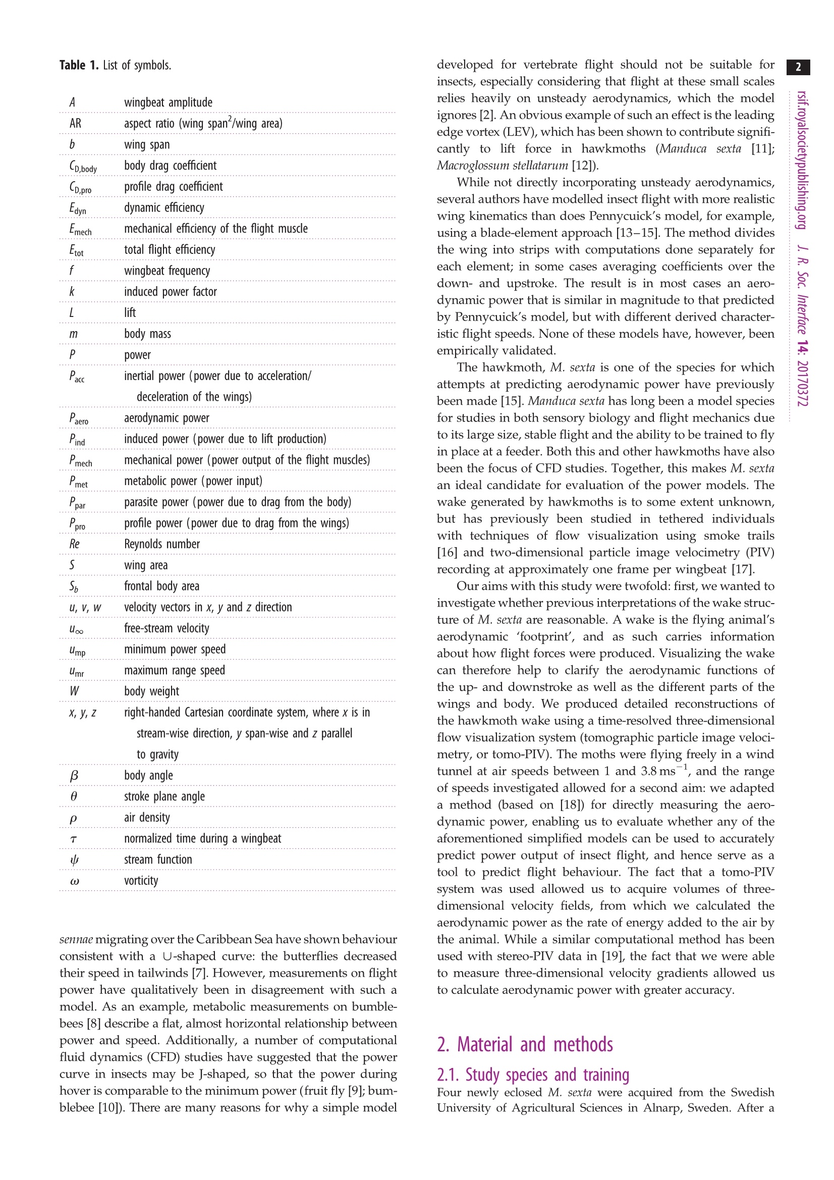
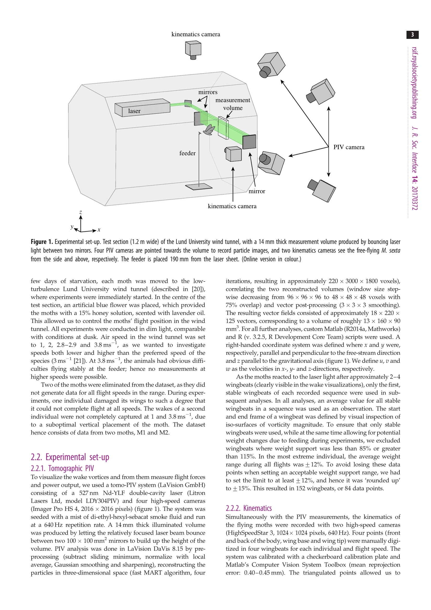
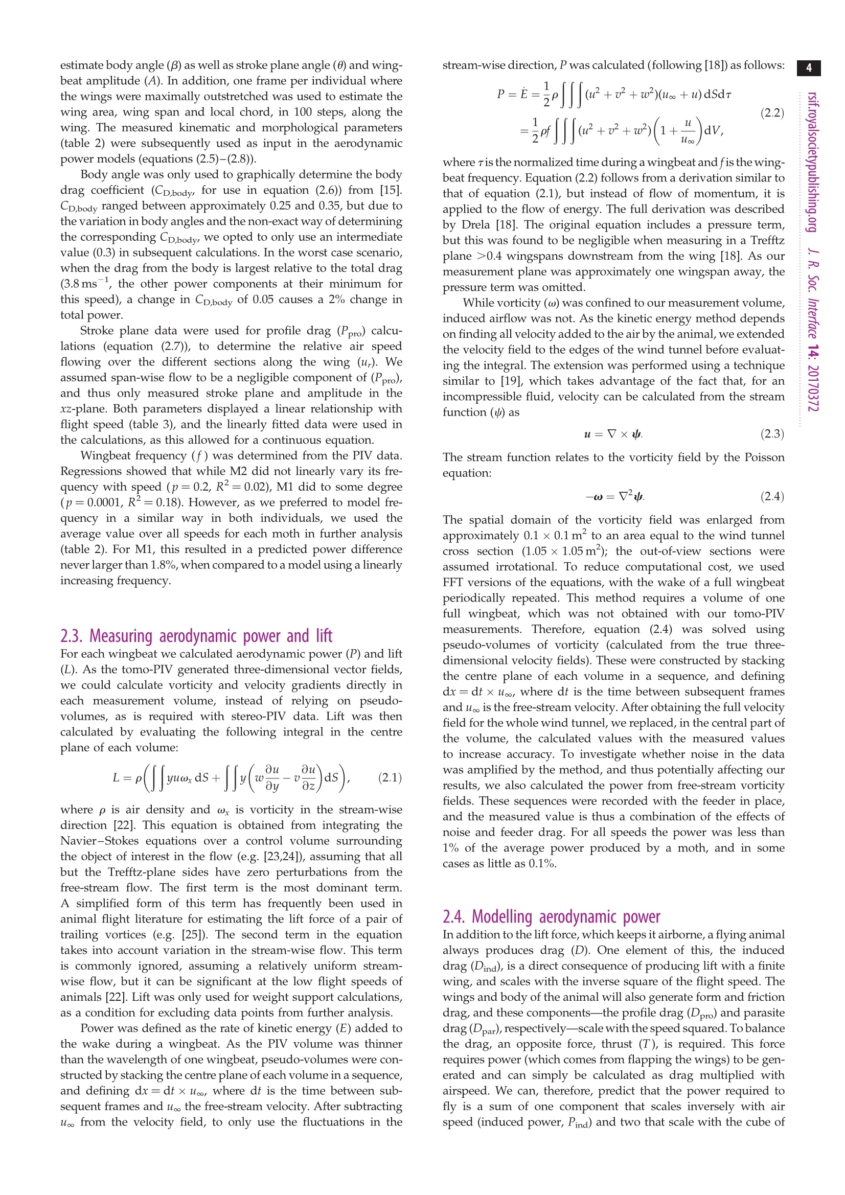
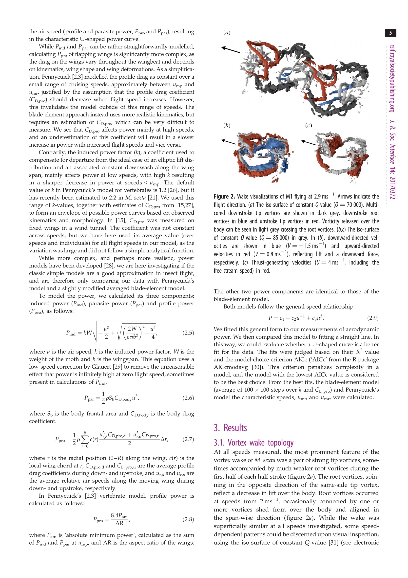
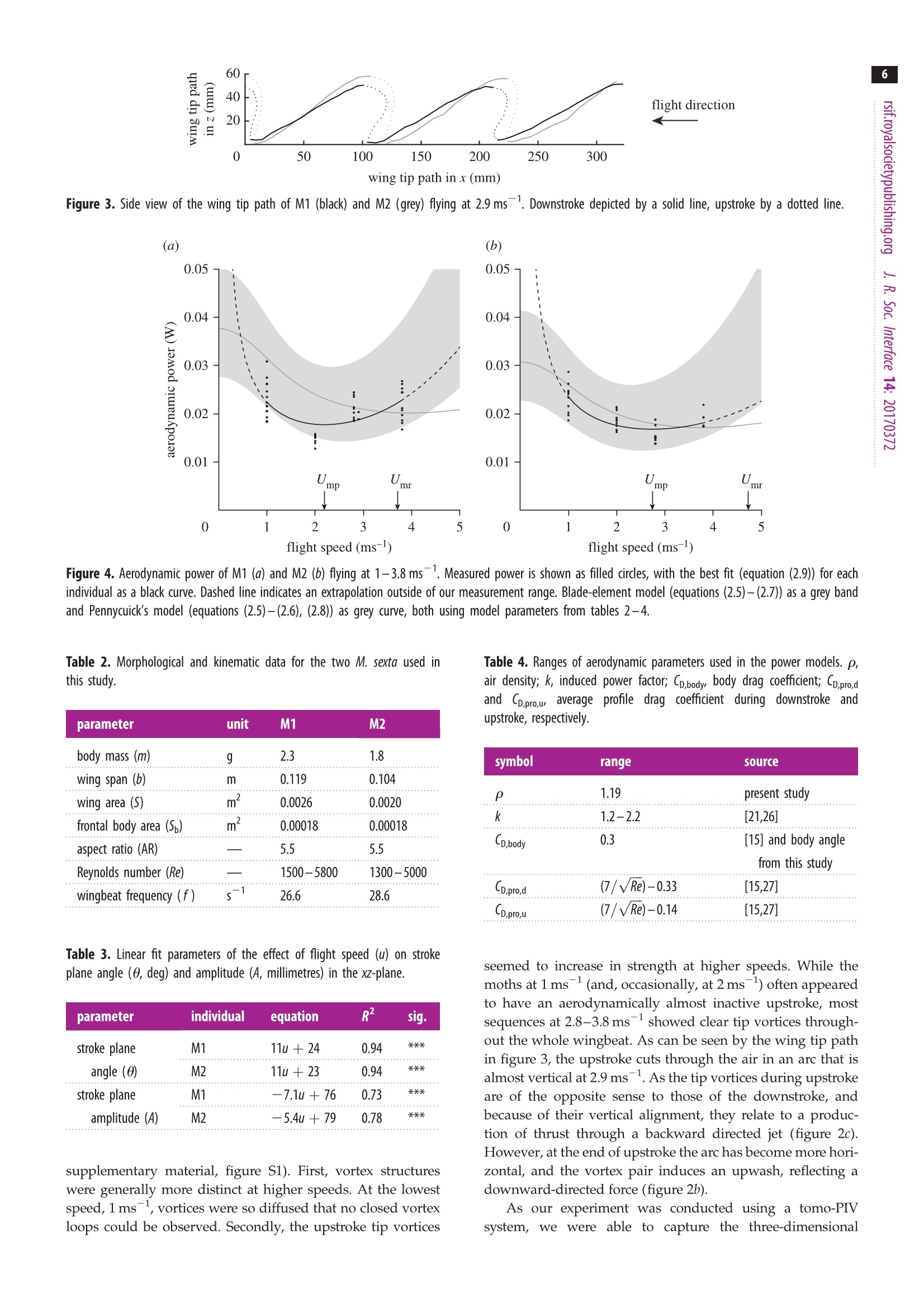
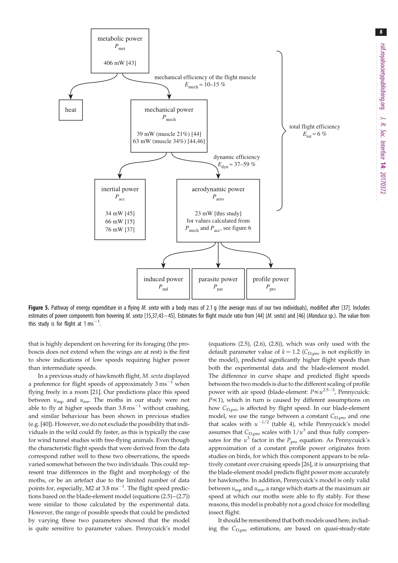
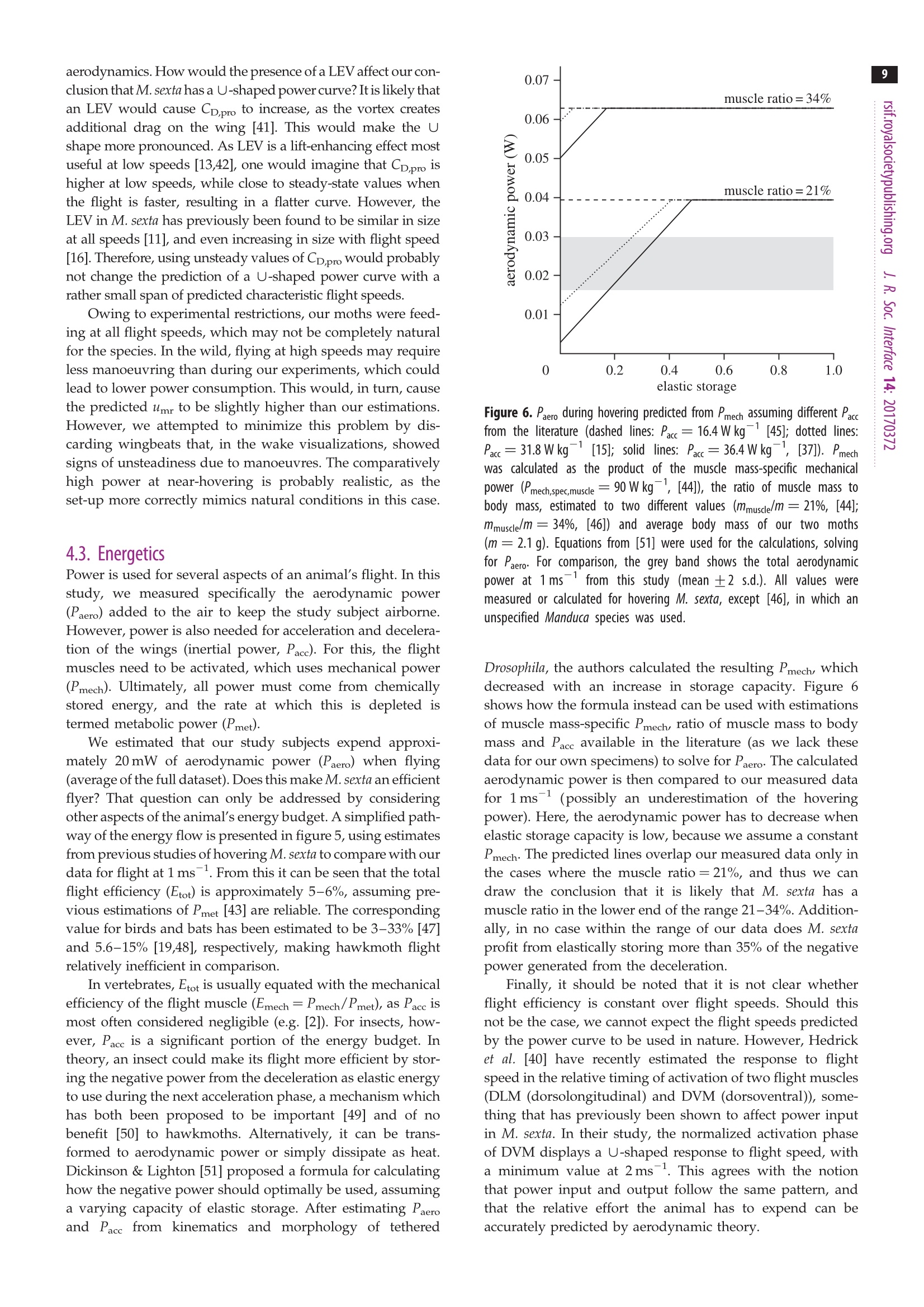
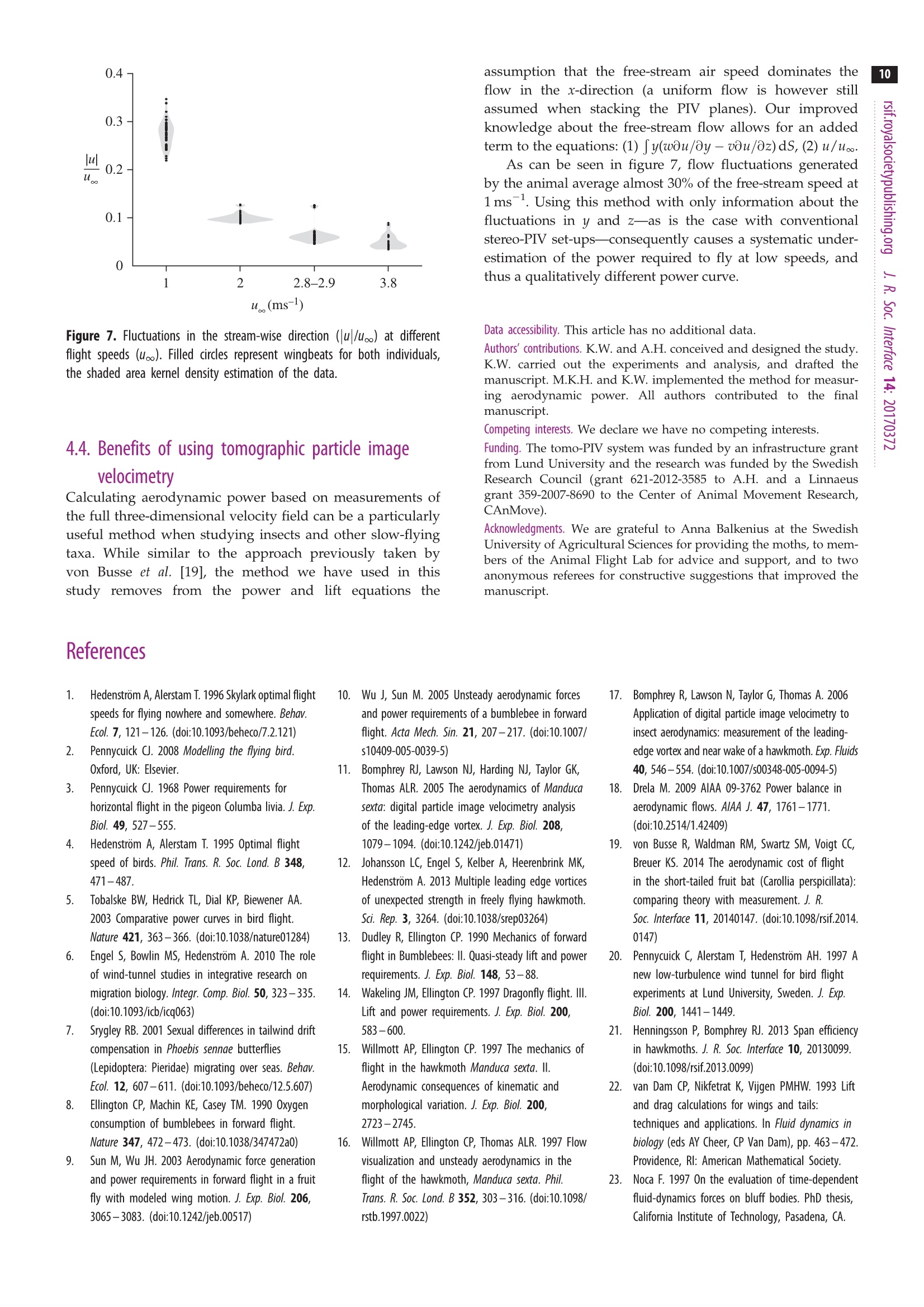
Table 1. List of symbols2 4 THE ROYAL SOCIETYPUBLISHINGC 2017 The Author(s) Published by the Royal Society. All rights reserved. INTERFACE rsif.royalsocietypublishing.org Research Check forupdates Cite this article： Warfvinge K，KleinHeerenbrink M， Hedenstrom A. 2017 The power-speed relationship is U-shaped intwo free-flying hawkmoths (Manduca sexta). J. R. Soc. Interface 14： 20170372. http：//dx.doi.org/10.1098/rsif.2017.0372 Keywords： Electronic supplementary material is availableonline at https：//dx.doi.org/10.6084/m9.figshare.c.3878398. The power-speed relationship isU-shaped in two free-flying hawkmoths(Manduca sexta) Kajsa Warfvingel， Marco KleinHeerenbrink1，2 and Anders Hedenstrom1 Department of Biology， Lund University， Lund， Sweden Department of Zoology， University of Oxford， Oxford， UK KW， 0000-0003-1038-8953； MK， 0000-0001-8172-8121； AH， 0000-0002-1757-0945 A flying animal can minimize its energy consumption by choosing an optimalflight speed depending on the task at hand. Choice of flight speed can be pre-dicted by modelling the aerodynamic power required for flight， and this toolhas previously been used extensively in bird migration research. For insects，however， it is uncertain whether any of the commonly used power modelsare useful， as insects often operate in a very different flow regime from ver-tebrates. To investigate this， we measured aerodynamic power in the wake oftwo Manduca sexta flying freely in a wind tunnel at 1-3.8 ms-， using tomo-graphic particle image velocimetry (tomo-PIV). The expended power wassimilar in magnitude to that predicted by two classic models. However， themost ubiquitously used model， originally intended for vertebrates， failed topredict the sharp increase in power at higher speeds，leading to an overestimateof predicted flight speed during longer flights. In addition to measuring aero-dynamic power， the tomo-PIV system yielded a highly detailed visualization ofthe wake， which proved to be significantly more intricate than could be inferredfrom previous smoke trail- and two-dimensional-PIV studies. 1. Introduction Flight is an energetically demanding method of locomotion. It is， therefore， natu-ral to assume that there is a selective pressure to economize power usage duringflight. There can be multiple optimization objectives， depending on the task athand： maximizing flight duration on a given energy budget is the aim when，e.g.， performing display flight [1]. In migration， or other longer flights， it maybe more beneficial to minimize the power per distance travelled [2]. If it is ofessence to arrive at the breeding grounds early to acquire a territory， time spenton migration is a reasonable currency to minimize. In all these examples， theoptimization strategy leads to a choice of flight speed， which can be predictedbased on how the power required to fly scales with flight speed. In the order men-tioned， these are the minimum power speed (ump)， maximum range speed (umr)and the optimal speed to minimize the time of migration (Umt) (table 1). In vertebrates， the flight speed-power relationship is often modelled as aU-shaped curve， defined by a number of morphological and kinematic parameters.The model was first adapted to bird flight from aeroplane theory by Pennycuick[2，3]， and its simplicity has allowed it to be ubiquitously used to， among otherthings， predict flight behaviour in migrating birds [4]. The flight speed-powerrelationship predicted from the model has， for bird flight， been qualitatively sup-ported by empirical data [5，6]. Some behaviours， such as responses to differentwind conditions， can be predicted by qualitative aspects of the model alone (theU shape). A testable example of this is the prediction that individuals choosingto fly at Umr should increase their speed in headwinds and decrease it in tailwinds，while behaving unaffected by wind when selecting ump [4]. Although Pennycuick’s model was originally created for vertebrates， thetheory behind a U-shaped power curve is in fact very general， and could， in prin-ciple， be applied also to other taxa， such as insects. Female (but not male) Phoebis A wingbeat amplitude sennae migrating over the Caribbean Sea have shown behaviourconsistent with a U-shaped curve： the butterflies decreasedtheir speed in tailwinds [7]. However， measurements on flightpower have qualitatively been in disagreement with such amodel. As an example， metabolic measurements on bumble-bees [8] describe a flat， almost horizontal relationship betweenpower and speed. Additionally， a number of computationalfluid dynamics (CFD) studies have suggested that the powercurve in insects may be J-shaped， so that the power duringhover is comparable to the minimum power (fruit fly [9]；bum-blebee [10]). There are many reasons for why a simple model developed for vertebrate flight should not be suitable forinsects， especially considering that flight at these small scalesrelies heavily on unsteady aerodynamics， which the modelignores [2]. An obvious example of such an effect is the leadingedge vortex (LEV)， which has been shown to contribute signifi-cantly to lift force in hawkmoths (Manduca sexta[11]；Macroglossum stellatarum [12]). While not directly incorporating unsteady aerodynamics，several authors have modelled insect flight with more realisticwing kinematics than does Pennycuick's model， for example，using a blade-element approach [13-15]. The method dividesthe wing into strips with computations done separately foreach element； in some cases averaging coefficients over thedown- and upstroke. The result is in most cases an aero-dynamic power that is similar in magnitude to that predictedby Pennycuick's model， but with different derived character-istic flight speeds. None of these models have， however， beenempirically validated. The hawkmoth， M. sexta is one of the species for whichattempts at predicting aerodynamic power have previouslybeen made [15]. Manduca sexta has long been a model speciesfor studies in both sensory biology and flight mechanics dueto its large size， stable flight and the ability to be trained to flyin place at a feeder. Both this and other hawkmoths have alsobeen the focus of CFD studies. Together， this makes M. sextaan ideal candidate for evaluation of the power models. Thewake generated by hawkmoths is to some extent unknown，but has previously been studied in tethered individualswith techniques of flow visualization using smoke trails[16] and two-dimensional particle image velocimetry (PIV)recording at approximately one frame per wingbeat [17]. Our aims with this study were twofold： first， we wanted toinvestigate whether previous interpretations of the wake struc-ture of M. sexta are reasonable. A wake is the flying animal'saerodynamic 'footprint'， and as such carries informationabout how flight forces were produced. Visualizing the wakecan therefore help to clarify the aerodynamic functions ofthe up- and downstroke as well as the different parts of thewings and body. We produced detailed reconstructions ofthe hawkmoth wake using a time-resolved three-dimensionalflow visualization system (tomographic particle image veloci-metry， or tomo-PIV). The moths were flying freely in a windtunnel at air speeds between 1 and 3.8 ms， and the rangeof speeds investigated allowed for a second aim： we adapteda method (based on [18]) for directly measuring the aero-dynamic power， enabling us to evaluate whether any of theaforementioned simplified models can be used to accuratelypredict power output of insect flight， and hence serve as atool to predict flight behaviour. The fact that a tomo-PIVsystem was used allowed us to acquire volumes of three-dimensional velocity fields， from which we calculated theaerodynamic power as the rate of energy added to the air bythe animal. While a similar computational method has beenused with stereo-PIV data in [19]， the fact that we were ableto measure three-dimensional velocity gradients allowed usto calculate aerodynamic power with greater accuracy. Figure 1. Experimental set-up. Test section (1.2 m wide) of the Lund University wind tunnel， with a 14 mm thick measurement volume produced by bouncing laserlight between two mirrors. Four PIV cameras are pointed towards the volume to record particle images， and two kinematics cameras see the free-flying M. sextafrom the side and above， respectively. The feeder is placed 190 mm from the laser sheet. (Online version in colour.) few days of starvation， each moth was moved to the low-turbulence Lund University wind tunnel (described in[20])，where experiments were immediately started. In the centre of thetest section， an artificial blue flower was placed， which providedthe moths with a 15% honey solution， scented with lavender oil.This allowed us to control the moths’ flight position in the windtunnel. All experiments were conducted in dim light， comparablewith conditions at dusk. Air speed in the wind tunnel was setto 1， 2， 2.8-2.9 and 3.8ms-， as we wanted to investigatespeeds both lower and higher than the preferred speed of thespecies (3ms-[21]). At 3.8 ms-l， the animals had obvious diffi-culties flying stably at the feeder； hence no measurements athigher speeds were possible. Two of the moths were eliminated from the dataset， as they didnot generate data for all flight speeds in the range. During exper-iments， one individual damaged its wings to such a degree thatit could not complete flight at all speeds. The wakes of a secondindividual were not completely captured at 1 and 3.8ms-1， dueto a suboptimal vertical placement of the moth. The datasethence consists of data from two moths， M1 and M2. 2.2. Experimental set-up 2.2.1. Tomographic PlV To visualize the wake vortices and from them measure flight forcesand power output， we used a tomo-PIV system (LaVision GmbH)consisting of a 527 nm Nd-YLF double-cavity laser (LitronLasers Ltd， model LDY304PIV) and four high-speed cameras(Imager Pro HS 4， 2016×2016 pixels)(figure 1). The system wasseeded with a mist of di-ethyl-hexyl-sebacat smoke fluid and runat a 640Hz repetition rate. A 14mm thick illuminated volumewas produced by letting the relatively focused laser beam bouncebetween two 100×100 mm² mirrors to build up the height of thevolume. PIV analysis was done in LaVision DaVis 8.15 by pre-processing (subtract sliding minimum， normalize with localaverage， Gaussian smoothing and sharpening)， reconstructing theparticles in three-dimensional space (fast MART algorithm， four iterations， resulting in approximately 220×3000×1800 voxels)，correlating the two reconstructed volumes (window size step-wise decreasing from 96×96×96 to 48×48×48 voxels with75% overlap) and vector post-processing (3×3×3 smoothing).The resulting vector fields consisted of approximately 18×220×125 vectors， corresponding to a volume of roughly 13×160×90mm. For all further analyses， custom Matlab (R2014a，Mathworks)and R (v. 3.2.5， R Development Core Team) scripts were used. ASWright-handed coordinate system was defined where x and y were，respectively，parallel and perpendicular to the free-stream directionand z parallel to the gravitational axis (figure 1). We define u， v andw as the velocities in x-， y-and z-directions， respectively. As the moths reacted to the laser light after approximately 2-4wingbeats (clearly visible in the wake visualizations)， only the first，stable wingbeats of each recorded sequence were used in sub-sequent analyses. In all analyses， an average value for all stablewingbeats in a sequence was used as an observation. The startand end frame of a wingbeat was defined by visual inspection ofiso-surfaces of vorticity magnitude. To ensure that only stablewingbeats were used， while at the same time allowing for potentialweight changes due to feeding during experiments， we excludedwingbeats where weight support was less than 85% or greaterthan 115%.In the most extreme individual， the average weightrange during all flights was ±12%. To avoid losing these datapoints when setting an acceptable weight support range， we hadto set the limit to at least ±12%， and hence it was rounded up'to ±15%. This resulted in 152 wingbeats， or 84 data points. 2.2.2. Kinematics Simultaneously with the PIV measurements， the kinematics ofthe flying moths were recorded with two high-speed cameras(HighSpeedStar 3， 1024×1024 pixels， 640 Hz). Four points (frontand back of the body， wing base and wing tip) were manually digi-tized in four wingbeats for each individual and flight speed. Thesystem was calibrated with a checkerboard calibration plate andMatlab’s Computer Vision System Toolbox (mean reprojectionerror： 0.40-0.45mm). The triangulated points allowed us to estimate body angle (B) as well as stroke plane angle (0) and wing-beat amplitude (A). In addition， one frame per individual wherethe wings were maximally outstretched was used to estimate thewing area， wing span and local chord， in 100 steps， along thewing. The measured kinematic and morphological parameters(table 2) were subsequently used as input in the aerodynamicpower models (equations (2.5)-(2.8)). Body angle was only used to graphically determine the bodydrag coefficient (CD，body， for use in equation (2.6)) from [15].CD，body ranged between approximately 0.25 and 0.35， but due tothe variation in body angles and the non-exact way of determiningthe corresponding CD，body， we opted to only use an intermediatevalue (0.3) in subsequent calculations. In the worst case scenario，when the drag from the body is largest relative to the total drag(3.8 ms， the other power components at their minimum forthis speed)， a change in CD，body of 0.05 causes a 2% change intotal power. Stroke plane data were used for profile drag (Ppro) calcu-lations (equation (2.7))， to determine the relative air speedflowing over the different sections along the wing (u). Weassumed span-wise flow to be a negligible component of (Ppro)，and thus only measured stroke plane and amplitude in thexz-plane. Both parameters displayed a linear relationship withflight speed (table 3)， and the linearly fitted data were used inthe calculations， as this allowed for a continuous equation. Wingbeat frequency (f) was determined from the PIV data.Regressions showed that while M2 did not linearly vary its fre-quency with speed(p=0.2， R2=0.02)， M1 did to some degree(p=0.0001， R²=0.18). However， as we preferred to model fre-quency in a similar way in both individuals， we used theaverage value over all speeds for each moth in further analysis(table 2). For M1， this resulted in a predicted power differencenever larger than 1.8%， when compared to a model using a linearlyincreasing frequency. 2.3. Measuring aerodynamic power and lift For each wingbeat we calculated aerodynamic power (P) and lift(L). As the tomo-PIV generated three-dimensional vector fields，we could calculate vorticity and velocity gradients directly ineach measurement volume， instead of relying on pseudo-volumes， as is required with stereo-PIV data. Lift was thencalculated by evaluating the following integral in the centreplane of each volume： where p is air density and wx is vorticity in the stream-wisedirection [22]. This equation is obtained from integrating theNavier-Stokes equations over a control volume surroundingthe object of interest in the flow (e.g. [23，24])， assuming that allbut the Trefftz-plane sides have zero perturbations from thefree-stream flow. The first term is the most dominant term.A simplified form of this term has frequently been used inanimal flight literature for estimating the lift force of a pair oftrailing vortices (e.g.[25]). The second term in the equationtakes into account variation in the stream-wise flow. This termis commonly ignored， assuming a relatively uniform stream-wise flow， but it can be significant at the low flight speeds ofanimals [22]. Lift was only used for weight support calculations，as a condition for excluding data points from further analysis. Power was defined as the rate of kinetic energy (E) added tothe wake during a wingbeat. As the PIV volume was thinnerthan the wavelength of one wingbeat， pseudo-volumes were con-structed by stacking the centre plane of each volume in a sequence，and defining dx= dt× uoo， where dt is the time between sub-sequent frames and u.. the free-stream velocity. After subtractingue from the velocity field， to only use the fluctuations in the where ris the normalized time during a wingbeat and fis thewing-beat frequency. Equation (2.2) follows from a derivation similar tothat of equation (2.1)， but instead of flow of momentum， it isapplied to the flow of energy. The full derivation was describedby Drela [18]. The original equation includes a pressure term，but this was found to be negligible when measuring in a Trefftzplane >0.4 wingspans downstream from the wing [18]. As ourmeasurement plane was approximately one wingspan away， thepressure term was omitted. While vorticity (w) was confined to our measurement volume，induced airflow was not. As the kinetic energy method dependson finding all velocity added to the air by the animal， we extendedthe velocity field to the edges of the wind tunnel beforeevaluat-ing the integral. The extension was performed using a techniquesimilar to [19]， which takes advantage of the fact that， for anincompressible fluid， velocity can be calculated from the streamfunction(w) as The stream function relates to the vorticity field by the Poissonequation： The spatial domain of the vorticity field was enlarged fromapproximately 0.1×0.1 m² to an area equal to the wind tunnelcross section (1.05×1.05 m²)； the out-of-view sections wereassumed irrotational. To reduce computational cost， we usedFFT versions of the equations， with the wake of a full wingbeatperiodically repeated. This method requires a volume of onefull wingbeat， which was not obtained with our tomo-PIVmeasurements. Therefore， equation (2.4)) was solved1 usingpseudo-volumes of vorticity (calculated from the true three-dimensional velocity fields). These were constructed by stackingthe centre plane of each volume in a sequence， and definingdx= dt× Uo， where dt is the time between subsequent framesand u is the free-stream velocity. After obtaining the full velocityfield for the whole wind tunnel， we replaced， in the central part ofthe volume， the calculated values with the measured valuesto increase accuracy. To investigate whether noise in the datawas amplified by the method， and thus potentially affecting ourresults， we also calculated the power from free-stream vorticityfields. These sequences were recorded with the feeder in place，and the measured value is thus a combination of the effects ofnoise and feeder drag. For all speeds the power was less than1% of the average power produced by a moth， and in somecases as little as 0.1%. 2.4. Modelling aerodynamic power In addition to the lift force， which keeps it airborne， a flying animalalways produces drag (D). One element of this， the induceddrag (Dind)， is a direct consequence of producing lift with a finitewing， and scales with the inverse square of the flight speed. Thewings and body of the animal will also generate form and frictiondrag， and these components-the profile drag (Dpro) and parasitedrag (Dpar)， respectively-scale with the speed squared. To balancethe drag， an opposite force， thrust (T)， is required. This forcerequires power (which comes from flapping the wings) to be gen-erated and can simply be calculated as drag multiplied withairspeed. We can， therefore， predict that the power required tofly is a sum of one component that scales inversely with airspeed (induced power， Pind) and two that scale with the cube of the air speed (profile and parasite power， Ppro and Ppar)， resultingin the characteristic U-shaped power curve. While Pind and Ppar can be rather straightforwardly modelled，calculating Ppro of flapping wings is significantly more complex， asthe drag on the wings vary throughout the wingbeat and dependson kinematics， wing shape and wing deformations. As a simplifica-tion， Pennycuick [2，3] modelled the profile drag as constant over asmall range of cruising speeds， approximately between ump andUmr justified by the assumption that the profile drag coefficient(CD，pro) should decrease when flight speed increases. However，this invalidates the model outside of this range of speeds. Theblade-element approach instead uses more realistic kinematics， butrequires an estimation of CDpro which can be very difficult tomeasure. We see that CD，pro affects power mainly at high speeds，and an underestimation of this coefficient will result in a slowerincrease in power with increased flight speeds and vice versa. Contrarily， the induced power factor (k)， a coefficient used tocompensate for departure from the ideal case of an elliptic lift dis-tribution and an associated constant downwash along the wingspan， mainly affects power at low speeds， with high k resultingin a sharper decrease in power at speeds

确定