


方案详情
文
采用LaVison的DaVis8.4软件平台和三台CMOS相机(Photron FastCAM SA1, 1 MegaPixel, 构成一套时间分辨3D3C抖盒子测量系统,并利用该系统进行了由大尺度PTV测量确定全尺寸骑车人模型的气动阻力的研究。
方案详情

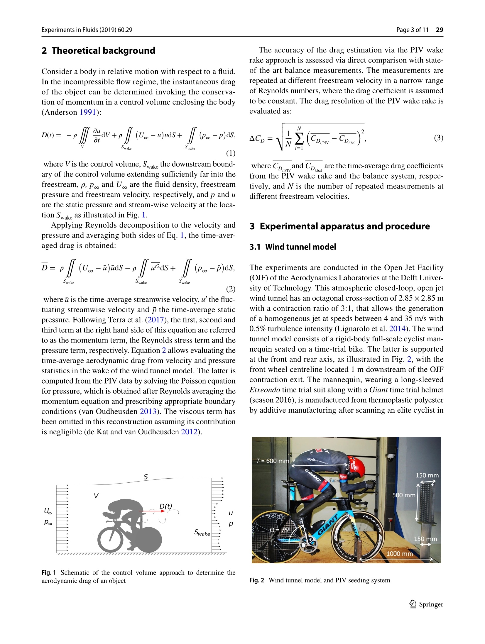
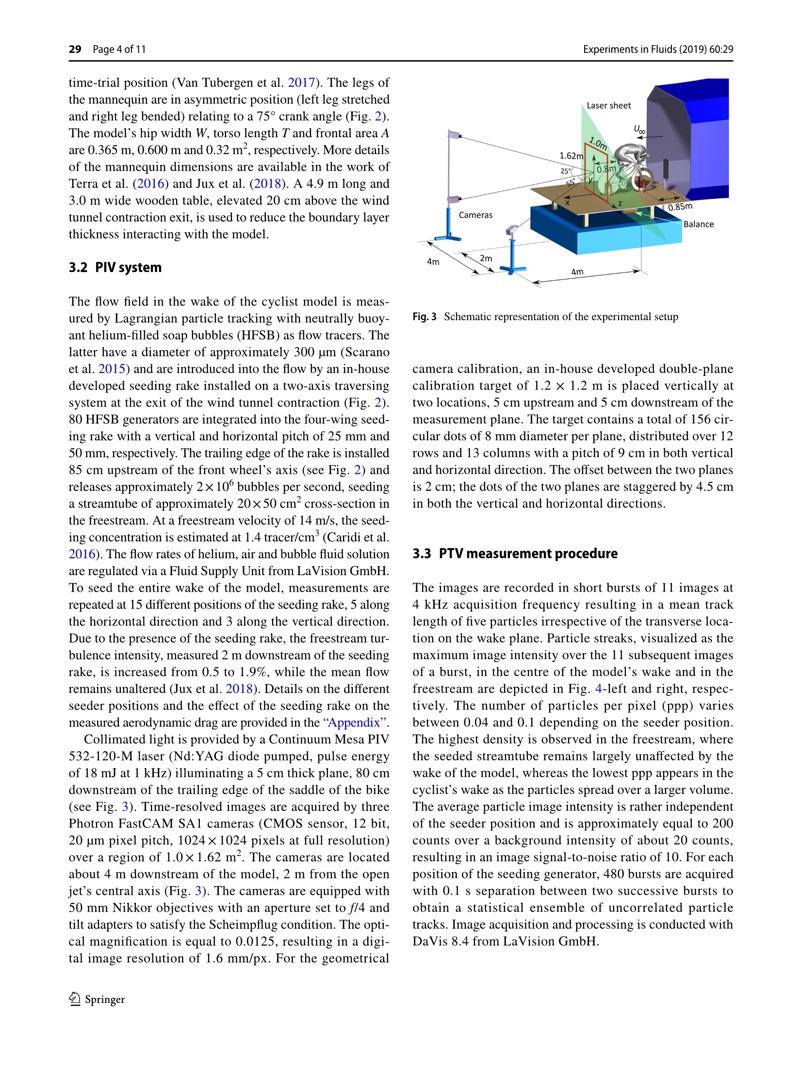
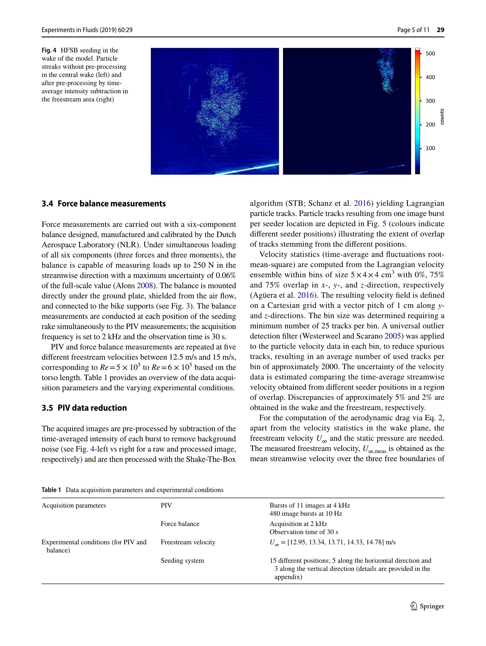
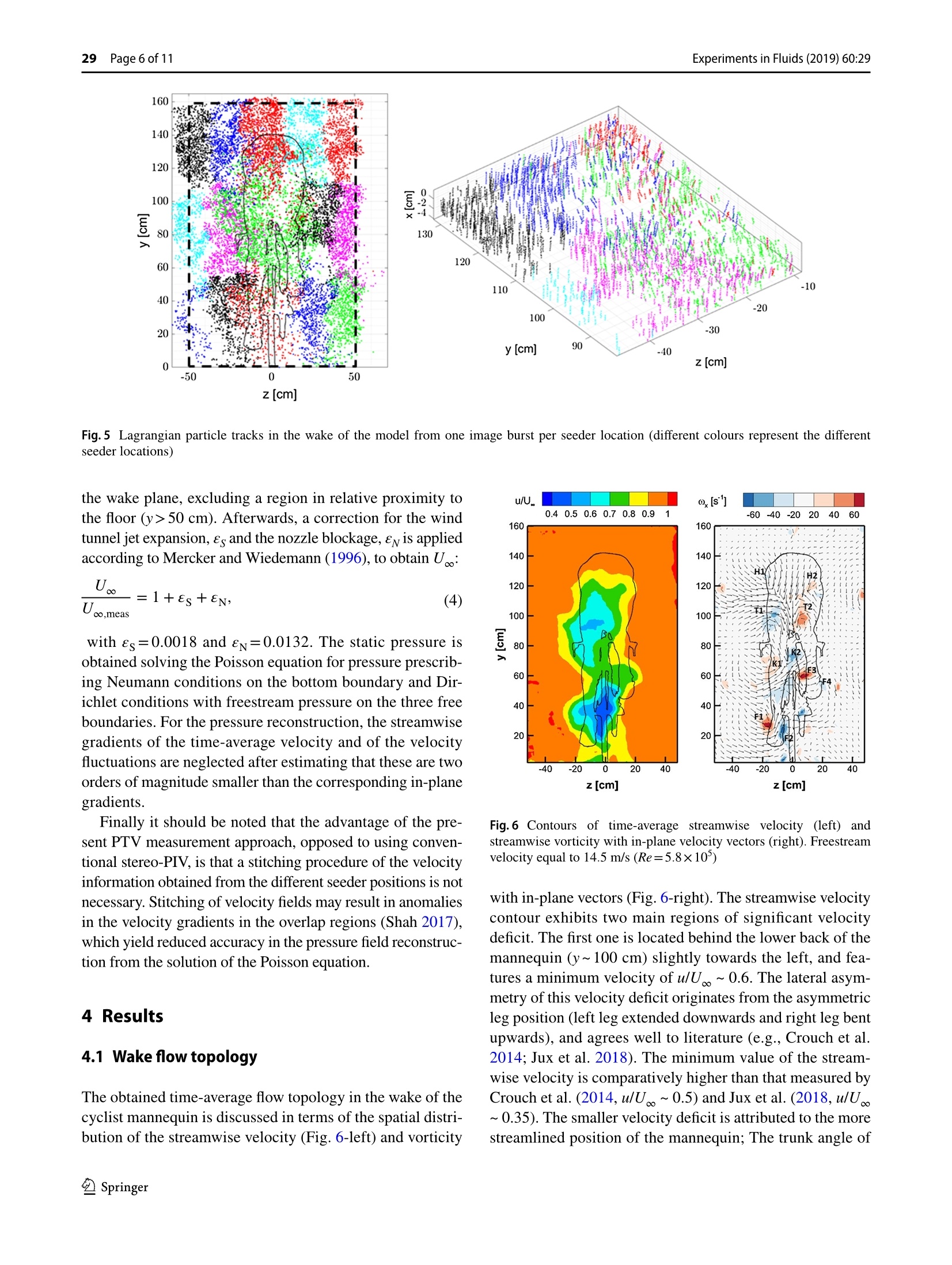
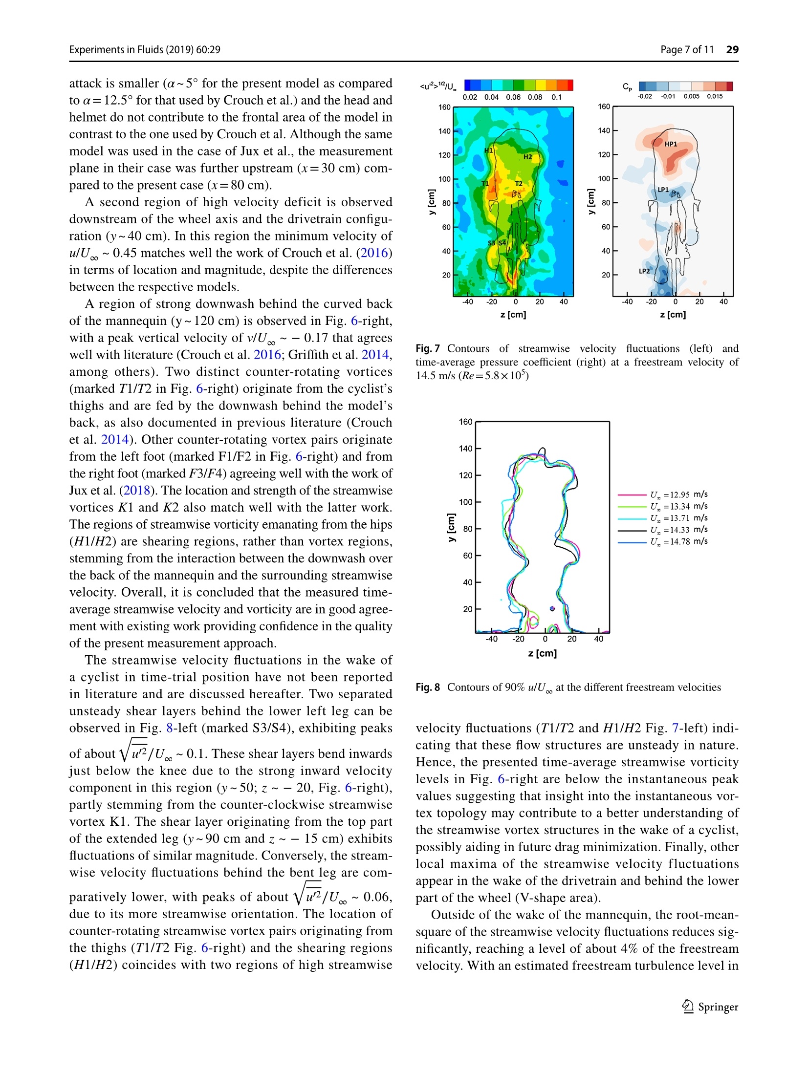
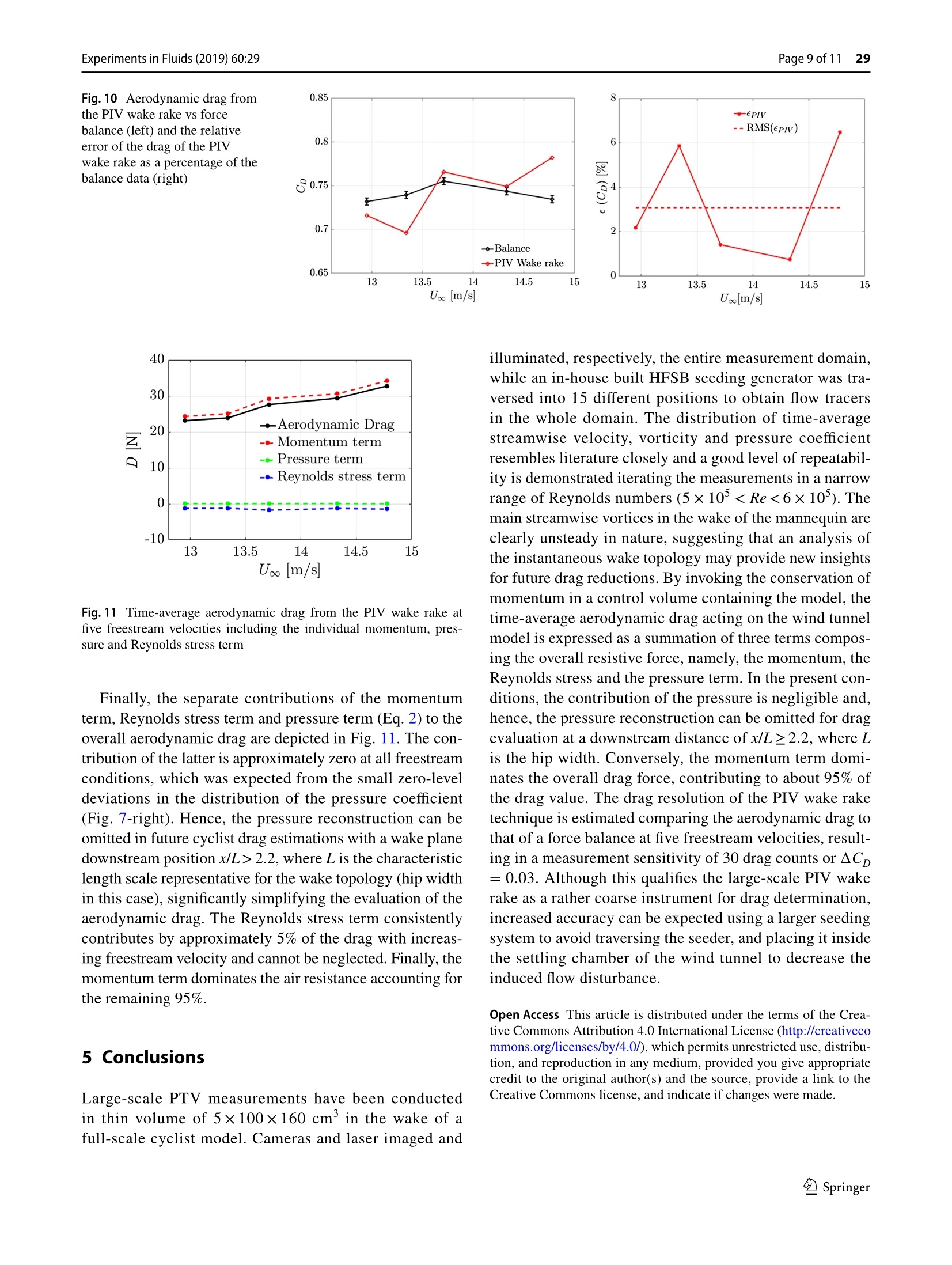
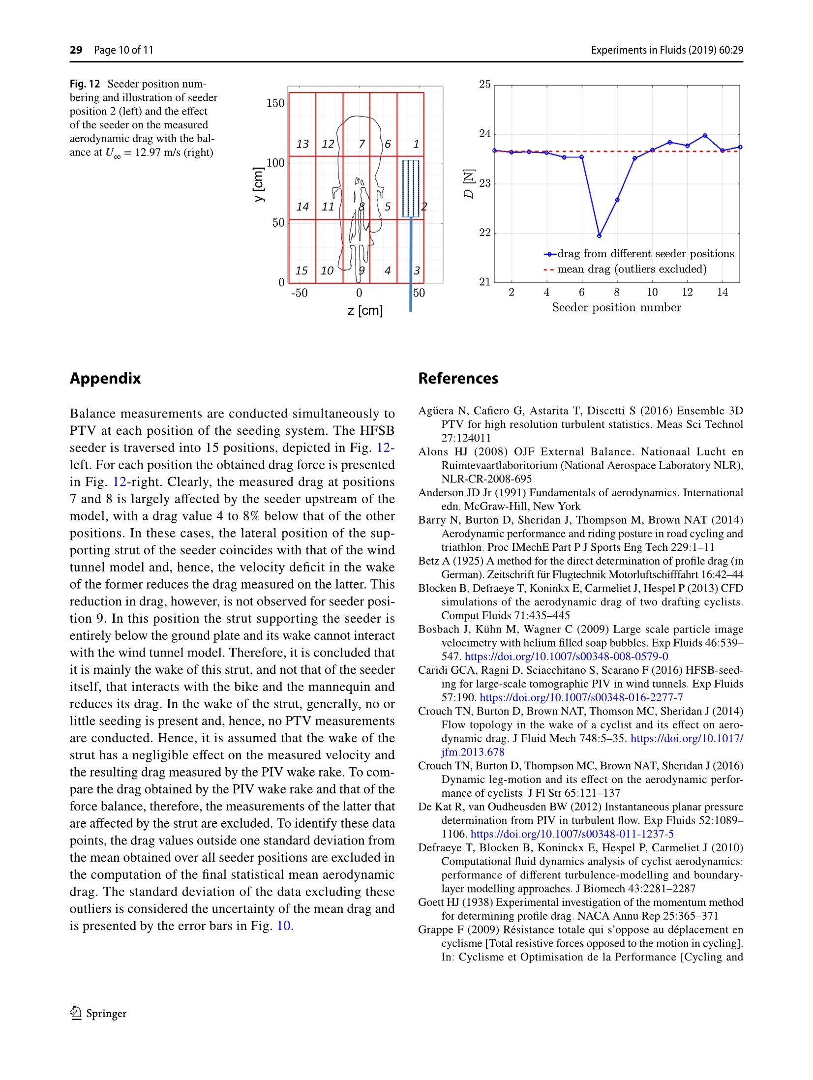
Experiments in Fluids (2019) 60:29https://doi.org/10.1007/s00348-019-2677-6 29 Page 2 of 11Experiments in Fluids (2019) 60:29 RESEARCH ARTICLE Aerodynamic drag determination of a full-scale cyclist mannequinfrom large-scale PTV measurements W.Terra1D.A. Sciacchitano1.Y.H.Shah1 Received: 23 August 2018/ Revised: 7 January 2019/ Accepted: 8 January 2019/ Published online:21 January 2019O The Author(s) 2019 Abstract The aerodynamic drag of a human-scale wind tunnel model is obtained from large-scale particle tracking velocimetrymeasurements invoking the conservation of momentum in a control volume surrounding the model. Lagrangian particletracking is employed to obtain the velocity and static pressure statistics in a thin volume in the wake of a cyclist mannequinat freestream velocities between 12.5 and 15 m/s, corresponding to Reynolds numbers from 5×10to 6×10 based onthe torso length. The spatial distributions of the time-average streamwise velocity and pressure coefficient match well withprevious works reported in literature. The streamwise velocity fluctuations in the wake of the cyclist’s model are presented,clearly demonstrating the unsteady nature of the main wake flow structures. Furthermore, the obtained aerodynamic dragfollows the expected quadratic increase with increasing freestream velocity. The accuracy of this drag estimation is evaluatedby comparison to force balance data and corresponds to 30 drag counts. The three terms composing the overall drag force,ascribed to the mean and fluctuating streamwise velocity and the mean pressure, are also evaluated separately, demonstratingthat the resistive force is dominated by the contribution of the mean streamwise momentum deficit, whereas the contributionof the pressure term is negligible. Graphical abstract Aerodynamic drag determination of a full-scale cyclistmannequin from large-scale PTV measurements The data presented in the figures in this work is available online(https://doi.org/10.4121/uuid:7f42e060-766d-4bf1-86c4-c648c794317c) 1 Introduction 区W.Terraw.terra@tudelft.n Aerospace Engineering Department, Delft Universityof Technology, Delft, The Netherlands Determination of the aerodynamic loads is relevant in manyfluid dynamic applications, e.g., for the fuel-efficient designof air and ground transportation systems, the safe structuraldesign of wind turbines and the maximization of perfor-mances in elite speed sports such as cycling and skating. Measurement of these aerodynamic loads is conventionallycarried out in wind tunnels, where full-scale or scaled-downmodels are immersed in a homogeneous stream of air, whilethe forces and moments are measured via six-componentforce balances (e.g.,Zdravkovich 1992; Tropea et al. 2007).Thanks to their high resolution (up to 0.0003% of the fullscale load, Tropea et al.2007) these balance systems arenowadays considered as standard tools especially for meas-urements in industrial wind tunnels. Nevertheless, such bal-ance measurements are regarded as “blind", in the sense thatthey do not provide insight in the flow field and flow struc-tures generating these aerodynamic loads. Alternatively,the aerodynamic loads can be evaluated using wake rakes,invoking the conservation of momentum across a controlvolume containing the model and measuring the total andstatic pressure in the wake of the model (Betz 1925; Jones1936; Goett 1938; Somers 1997, among others). In contrastto balance measurements, the wake rake approach providesnot only the aerodynamic forces, but also allows relatingthese forces to the flow variables in the wake of the model.yielding a deeper insight into the components and genera-tion of the total resistive force (e.g., Maskell 1973; Huchoand Sovran 1993). These pressure-based wake rake measure-ments, however, are intrusive in nature and yield the resultat a single point in space, requiring traversing mechanismsand precluding measurement of the instantaneous flow field. In the last two decades Particle Image Velocimetry(PIV) has been used extensively as a viable alternativeto the pressure probe wake rakes, for loads determinationfrom wake velocity data, primarily due to its whole-fieldmeasurement capability and non-intrusive nature. Lin andRockwell (1996) and Unal et al. (1997) conducted PIVmeasurements in the wake of a two-dimensional cylinderto characterize its unsteady lift coefficient at Re=3780.Similarly, Noca et al. (1997) and Kurtulus et al. (2007)used time-resolved PIV to quantify the unsteady aero-dynamic forces of cylinders at Re=100 and Re=4890,respectively. Using PIV velocity data and the control vol-ume approach, van Oudheusden et al. (2006) character-ized the time-average aerodynamic forces and pitchingmoment of an airfoil; the authors reported a discrepancybetween the drag coefficient measured with the PIV wakerake and the conventional pressure-based wake rake of 1drag count (or ACp=10). Ragni et al. (2009) proved thefeasibility of the PIV wake rake for drag determination ofa transonic airfoil at Mach=0.6. In a successive work, theauthors extended the use of the PIV wake rake to movingobjects for the determination of the aerodynamic loads onan aircraft propeller blade (Ragni et al. 2011). Recently,a detailed review of loads estimation approaches fromPIV measurements has been carried out by Rival and vanOudheusden (2017) and a set of guidelines is provided for accurate fluid force measurements involving unsteadybody motion by Lentink (2018). Despite the popularity of the PIV wake rake for meas-uring the time-average and instantaneous loads and inves-tigation of the governing flow fields, its application hasbeen limited to relatively small sized wind tunnel models(typical characteristic length of the order of 10 cm) dueto the limited domain of conventional PIV measurements(Raffel et al. 2018). This is largely ascribed to the lowscattering efficiency of conventional micrometric flowtracers. The introduction of sub-millimeter Helium-filledsoap bubbles (HFSB) as flow tracers for PIV measure-ments (Bosbach et al.2009; Scarano et al. 2015) allowed adramatic increase in measurement size (square meters andliters for planar and volumetric PIV, respectively), making‘large-scale'PIV measurements possible in wind tunnels.Large-scale PIV has mainly been exploited for volumetricPIV measurements. Caridi et al.(2016) made use of large-scale tomographic PIV over a volume of 12 1 to investigatethe flow field at the tip of a vertical axis wind turbineblade. By conducting large-scale PTV measurements andsolving the Poisson equation for pressure, Schneiders et al.(2016) measured the instantaneous volumetric pressure inthe wake of a truncated cylinder over a volume of about6 liters. Loads determination from large-scale PIV hasbeen attempted for the first time by Terra et al. (2017),estimating the drag coefficient of a transiting sphere atRe=10,000. Load determination from large-scale PIVin wind tunnels, however, has been hampered firstly bythe limited HFSB tracers concentration, which has beenbelow 1 bubble/cm’ (Caridi et al. 2016), and secondly bythe limited size of the seeded stream tube cross-section.not exceeding the order of 0.1 m²(Caridi et al. 2016; Juxet al. 2018). The present work aims to assess the feasibility of usinga large-scale PIV wake rake for the determination of theaerodynamic drag on a three-dimensional human-scalewind tunnel model. For this purpose,Lagrangian particletracking is employed to obtain the velocity in a plane ofapproximately 1.6 m’ in the wake of a full-scale cyclist man-nequin, demonstrating the human-scale PIV wake rake on afully three-dimensional, unsteady and highly complex flow,recently discussed in several studies (Defraeye et al. 2010;Crouch et al. 2014; Barry et al. 2014, among others). Theobtained time-average flow topology is presented and vali-dated against literature. Furthermore, for the first time thedistribution of streamwise velocity fluctuations and experi-mentally measured pressure in the wake plane are presentedand discussed. Finally, the accuracy of the aerodynamic dragis evaluated by comparison with state-of-the-art balancemeasurements and repeating the measurements at varyingfreestream velocity. 2 Theoretical background Consider a body in relative motion with respect to a fluid.In the incompressible flow regime, the instantaneous dragof the object can be determined invoking the conserva-tion of momentum in a control volume enclosing the body(Anderson 1991): where Vis the control volume, Swake the downstream bound-ary of the control volume extending sufficiently far into thefreestream, p,P and U are the fluid density, freestreampressure and freestream velocity, respectively, and p and uare the static pressure and stream-wise velocity at the loca-tion Swake as illustrated in Fig. 1. Applying Reynolds decomposition to the velocity andpressure and averaging both sides of Eq. 1, the time-aver-aged drag is obtained: where u is the time-average streamwise velocity, u'the fluc-tuating streamwise velocity and p the time-average staticpressure. Following Terra et al. (2017), the first, second andthird term at the right hand side of this equation are referredto as the momentum term, the Reynolds stress term and thepressure term, respectively. Equation 2 allows evaluating thetime-average aerodynamic drag from velocity and pressurestatistics in the wake of the wind tunnel model. The latter iscomputed from the PIV data by solving the Poisson equationfor pressure, which is obtained after Reynolds averaging themomentum equation and prescribing appropriate boundaryconditions (van Oudheusden 2013). The viscous term hasbeen omitted in this reconstruction assuming its contributionis negligible (de Kat and van Oudheusden 2012). Fig. 1 Schematic of the control volume approach to determine theaerodynamic drag of an object The accuracy of the drag estimation via the PIV wakerake approach is assessed via direct comparison with state-of-the-art balance measurements. The measurements arerepeated at different freestream velocity in a narrow rangeof Reynolds numbers, where the drag coefficient is assumedto be constant. The drag resolution of the PIV wake rake isevaluated as: where CDp and CDita are the time-average drag coefficientsfrom the PIV wake rake and the balance system, respec-tively, and N is the number of repeated measurements atdifferent freestream velocities. 3 Experimental apparatus and procedure 3.1 Wind tunnel model The experiments are conducted in the Open Jet Facility(OJF) of the Aerodynamics Laboratories at the Delft Univer-sity of Technology. This atmospheric closed-loop, open jetwind tunnel has an octagonal cross-section of 2.85×2.85 mwith a contraction ratio of 3:1, that allows the generationof a homogeneous jet at speeds between 4 and 35 m/s with0.5% turbulence intensity (Lignarolo et al. 2014). The windtunnel model consists of a rigid-body full-scale cyclist man-nequin seated on a time-trial bike. The latter is supportedat the front and rear axis, as illustrated in Fig.2, with thefront wheel centreline located 1 m downstream of the OJFcontraction exit. The mannequin, wearing a long-sleevedEtxeondo time trial suit along with a Giant time trial helmet(season 2016), is manufactured from thermoplastic polyesterby additive manufacturing after scanning an elite cyclist in Fig.2 Wind tunnel model and PIV seeding system time-trial position (Van Tubergen et al. 2017). The legs ofthe mannequin are in asymmetric position (left leg stretchedand right leg bended) relating to a 75° crank angle (Fig. 2).The model’s hip width W, torso length T and frontal area Aare 0.365 m, 0.600 m and 0.32 m, respectively. More detailsof the mannequin dimensions are available in the work ofTerra et al. (2016) and Jux et al. (2018). A 4.9 m long and3.0 m wide wooden table,elevated 20 cm above the windtunnel contraction exit, is used to reduce the boundary layerthickness interacting with the model. 3.2 PIV system The flow field in the wake of the cyclist model is meas-ured by Lagrangian particle tracking with neutrally buoy-ant helium-filled soap bubbles (HFSB) as flow tracers. Thelatter have a diameter of approximately 300 um (Scaranoet al. 2015) and are introduced into the flow by an in-housedeveloped seeding rake installed on a two-axis traversingsystem at the exit of the wind tunnel contraction (Fig. 2).80 HFSB generators are integrated into the four-wing seed-ing rake with a vertical and horizontal pitch of 25 mm and50 mm, respectively. The trailing edge of the rake is installed85 cm upstream of the front wheel’s axis (see Fig. 2) andreleases approximately 2×10°bubbles per second,seedinga streamtube of approximately 20×50 cmcross-section inthe freestream. At a freestream velocity of 14 m/s, the seed-ing concentration is estimated at 1.4 tracer/cm’(Caridi et al.2016). The flow rates of helium, air and bubble fluid solutionare regulated via a Fluid Supply Unit from LaVision GmbH.To seed the entire wake of the model, measurements arerepeated at 15 different positions of the seeding rake, 5 alongthe horizontal direction and 3 along the vertical direction.Due to the presence of the seeding rake, the freestream tur-bulence intensity, measured 2 m downstream of the seedingrake, is increased from 0.5 to 1.9%, while the mean flowremains unaltered (Jux et al. 2018). Details on the differentseeder positions and the effect of the seeding rake on themeasured aerodynamic drag are provided in the“Appendix”. Collimated light is provided by a Continuum Mesa PIV532-120-M laser (Nd:YAG diode pumped, pulse energyof 18 mJ at 1 kHz) illuminating a 5 cm thick plane, 80 cmdownstream of the trailing edge of the saddle of the bike(see Fig.3). Time-resolved images are acquired by threePhotron FastCAM SA1 cameras (CMOS sensor, 12 bit,20 um pixel pitch, 1024×1024 pixels at full resolution)over a region of 1.0×1.62m². The cameras are locatedabout 4 m downstream of the model, 2 m from the openjet’s central axis (Fig.3). The cameras are equipped with50 mm Nikkor objectives with an aperture set to f/4 andtilt adapters to satisfy the Scheimpflug condition. The opti-cal magnification is equal to 0.0125, resulting in a digi-tal image resolution of 1.6 mm/px. For the geometrical Fig. 3 Schematic representation of the experimental setup camera calibration, an in-house developed double-planecalibration target of 1.2 × 1.2 m is placed vertically attwo locations, 5 cm upstream and 5 cm downstream of themeasurement plane. The target contains a total of 156 cir-cular dots of 8 mm diameter per plane, distributed over 12rows and 13 columns with a pitch of 9 cm in both verticaland horizontal direction. The offset between the two planesis 2 cm; the dots of the two planes are staggered by 4.5 cmin both the vertical and horizontal directions. 3.3 PTVmeasurement procedure The images are recorded in short bursts of 11 images at4 kHz acquisition frequency resulting in a mean tracklength of five particles irrespective of the transverse loca-tion on the wake plane. Particle streaks, visualized as themaximum image intensity over the 11 subsequent imagesof a burst, in the centre of the model’s wake and in thefreestream are depicted in Fig. 4-left and right, respec-tively. The number of particles per pixel (ppp) variesbetween 0.04 and 0.1 depending on the seeder position.The highest density is observed in the freestream, wherethe seeded streamtube remains largely unaffected by thewake of the model, whereas the lowest ppp appears in thecyclist’s wake as the particles spread over a larger volume.The average particle image intensity is rather independentof the seeder position and is approximately equal to 200counts over a background intensity of about 20 counts,resulting in an image signal-to-noise ratio of 10. For eachposition of the seeding generator, 480 bursts are acquiredwith 0.1 s separation between two successive bursts toobtain a statistical ensemble of uncorrelated particletracks. Image acquisition and processing is conducted withDaVis 8.4 from LaVision GmbH. Fig. 4 HFSB seeding in thewake of the model. Particlestreaks without pre-processingin the central wake (left) andafter pre-processing by time-average intensity subtraction inthe freestream area (right) 500 400 300 200 100 Force measurements are carried out with a six-componentbalance designed, manufactured and calibrated by the DutchAerospace Laboratory (NLR). Under simultaneous loadingof all six components (three forces and three moments), thebalance is capable of measuring loads up to 250 N in thestreamwise direction with a maximum uncertainty of 0.06%of the full-scale value (Alons 2008). The balance is mounteddirectly under the ground plate, shielded from the air flow,and connected to the bike supports (see Fig. 3). The balancemeasurements are conducted at each position of the seedingrake simultaneously to the PIV measurements; the acquisitionfrequency is set to 2 kHz and the observation time is 30 s. PIV and force balance measurements are repeated at fivedifferent freestream velocities between 12.5 m/s and 15 m/s,corresponding to Re=5×10to Re=6×10° based on thetorso length. Table 1 provides an overview of the data acqui-sition parameters and the varying experimental conditions. 3.5 PIV data reduction The acquired images are pre-processed by subtraction of thetime-averaged intensity of each burst to remove backgroundnoise (see Fig. 4-left vs right for a raw and processed image,respectively) and are then processed with the Shake-The-Box Table 1 Data acquisition parameters and experimental conditions Acquisition parameters PIV Bursts of 11 images at 4 kHz Experimental conditions (for PIV and balance) 480 image bursts at 10 Hz Force balance Acquisition at 2 kHz Observation time of 30 s Freestream velocity U=[12.95,13.34,13.71,14.33, 14.78] m/s Seeding system 15 different positions; 5 along the horizontal direction and 3 along the vertical direction (details are provided in the appendix) algorithm (STB; Schanz et al. 2016) yielding Lagrangianparticle tracks. Particle tracks resulting from one image burstper seeder location are depicted in Fig. 5 (colours indicatedifferent seeder positions) illustrating the extent of overlapof tracks stemming from the different positions. Velocity statistics (time-average and fluctuations root-mean-square) are computed from the Lagrangian velocityensemble within bins of size 5×4×4 cm’with 0%, 75%and 75% overlap in x-, y-, and z-direction, respectively(Agiiera et al. 2016). The resulting velocity field is definedon a Cartesian grid with a vector pitch of 1 cm along y-and z-directions. The bin size was determined requiring aminimum number of 25 tracks per bin. A universal outlierdetection filter (Westerweel and Scarano 2005) was appliedto the particle velocity data in each bin, to reduce spurioustracks, resulting in an average number of used tracks perbin of approximately 2000. The uncertainty of the velocitydata is estimated comparing the time-average streamwisevelocity obtained from different seeder positions in a regionof overlap. Discrepancies of approximately 5% and 2% areobtained in the wake and the freestream, respectively. For the computation of the aerodynamic drag via Eq. 2,apart from the velocity statistics in the wake plane, thefreestream velocity U and the static pressure are needed.The measured freestream velocity, Uco,meas is obtained as themean streamwise velocity over the three free boundaries of the wake plane, excluding a region in relative proximity tothe floor (y>50 cm). Afterwards, a correction for the windtunnel jet expansion, Eg and the nozzle blockage, ev is appliedaccording to Mercker and Wiedemann (1996), to obtain U: with es=0.0018 and eN=0.0132. The static pressure isobtained solving the Poisson equation for pressure prescrib-ing Neumann conditions on the bottom boundary and Dir-ichlet conditions with freestream pressure on the three freeboundaries. For the pressure reconstruction, the streamwisegradients of the time-average velocity and of the velocityfluctuations are neglected after estimating that these are twoorders of magnitude smaller than the corresponding in-planegradients. Finally it should be noted that the advantage of the pre-sent PTV measurement approach, opposed to using conventional stereo-PIV, is that a stitching procedure of the velocityinformation obtained from the different seeder positions is notnecessary. Stitching of velocity fields may result in anomaliesin the velocity gradients in the overlap regions (Shah 2017),which yield reduced accuracy in the pressure field reconstruc-tion from the solution of the Poisson equation. 4 Results 4.1 Wake flow topology The obtained time-average flow topology in the wake of thecyclist mannequin is discussed in terms of the spatial distri-bution of the streamwise velocity (Fig.6-left) and vorticity Fig.5 Lagrangian particle tracks in the wake of the mode from one image burst per seeder location (different colours represent the differentseeder locations) Fig.6 Contours of time-average streamwise velocity (left))2andstreamwise vorticity with in-plane velocity vectors (right). Freestreamvelocity equal to 14.5 m/s (Re=5.8×10) with in-plane vectors (Fig.6-right). The streamwise velocitycontour exhibits two main regions of significant velocitydeficit. The first one is located behind the lower back of themannequin (y~100 cm) slightly towards the left, and fea-tures a minimum velocity of u/U。~0.6. The lateral asym-metry of this velocity deficit originates from the asymmetricleg position (left leg extended downwards and right leg bentupwards), and agrees well to literature (e.g., Crouch et al.2014; Jux et al. 2018). The minimum value of the stream-wise velocity is comparatively higher than that measured byCrouch et al.(2014, u/U.。~0.5) and Jux et al. (2018, u/U~0.35). The smaller velocity deficit is attributed to the morestreamlined position of the mannequin; The trunk angle of attack is smaller(α~5° for the present model as comparedto a=12.5°for that used by Crouch et al.) and the head andhelmet do not contribute to the frontal area of the model incontrast to the one used by Crouch et al. Although the samemodel was used in the case of Jux et al., the measurementplane in their case was further upstream (x=30 cm) com-pared to the present case (x=80 cm). A second region of high velocity deficit is observeddownstream of the wheel axis and the drivetrain configu-ration (y~40 cm). In this region the minimum velocity ofu/U。~ 0.45 matches well the work of Crouch et al.(2016)in terms of location and magnitude, despite the differencesbetween the respective models. A region of strong downwash behind the curved backof the mannequin (y~120 cm) is observed in Fig. 6-right,with a peak vertical velocity of v/U。~- 0.17 that agreeswell with literature (Crouch et al. 2016; Griffith et al. 2014,among others). Two distinct counter-rotating vortices(marked T1/T2 in Fig. 6-right) originate from the cyclist’sthighs and are fed by the downwash behind the model’sback, as also documented in previous literature (Crouchet al.2014). Other counter-rotating vortex pairs originatefrom the left foot (marked F1/F2 in Fig. 6-right) and fromthe right foot (marked F3/F4) agreeing well with the work ofJux et al. (2018). The location and strength of the streamwisevortices K1 and K2 also match well with the latter work.The regions of streamwise vorticity emanating from the hips(H1/H2) are shearing regions, rather than vortex regions,stemming from the interaction between the downwash overthe back of the mannequin and the surrounding streamwisevelocity. Overall, it is concluded that the measured time-average streamwise velocity and vorticity are in good agree-ment with existing work providing confidence in the qualityof the present measurement approach. The streamwise velocity fluctuations in the wake ofa cyclist in time-trial position have not been reportedin literature and are discussed hereafter. Two separatedunsteady shear layers behind the lower left leg can beobserved in Fig. 8-left (marked S3/S4), exhibiting peaks of about Vur/U.。~ 0.1. These shear layers bend inwardsjust below the knee due to the strong inward velocitycomponent in this region (y~50; z~-20, Fig. 6-right),partly stemming from the counter-clockwise streamwisevortex K1. The shear layer originating from the top partof the extended leg (y~90 cm and z ~ - 15 cm) exhibitsfluctuations of similar magnitude. Conversely, the stream-wise velocity fluctuations behind the bent leg are com- paratively lower, with peaks of about Vu2/U..~0.06,due to its more streamwise orientation. The location ofcounter-rotating streamwise vortex pairs originating fromthe thighs (T1/T2 Fig. 6-right) and the shearing regions(H1/H2) coincides with two regions of high streamwise Fig.7 Contours01ofstreamwisevelocity fluctuations ((left)) andtime-average pressure coefficient (right) at a freestream velocity of14.5 m/s (Re=5.8×10) Fig. 8 Contours of 90% u/U at the different freestream velocities velocity fluctuations (T1/T2 and H1/H2 Fig. 7-left) indi-cating that these flow structures are unsteady in nature.Hence, the presented time-average streamwise vorticitylevels in Fig. 6-right are below the instantaneous peakvalues suggesting that insight into the instantaneous vor-tex topology may contribute to a better understanding ofthe streamwise vortex structures in the wake of a cyclist,possibly aiding in future drag minimization. Finally, otherlocal maxima of the streamwise velocity fluctuationsappear in the wake of the drivetrain and behind the lowerpart of the wheel (V-shape area). Outside of the wake of the mannequin, the root-mean-square of the streamwise velocity fluctuations reduces sig-nificantly, reaching a level of about 4% of the freestreamvelocity. With an estimated freestream turbulence level in the wake of the seeding system of 1.9% (Jux et al. 2018), itis argued that the freestream turbulence intensity is likelyoverestimated due to measurement random errors of thelarge-scale PTV system. As a consequence, the contribu-tion of the Reynolds stress term in the expression for thedrag (second term in Eq. 2) is overestimated, thus yieldingan underestimation of the aerodynamic drag by approxi-mately 0.15 N. At sufficient distance behind a bluff body, the contribu-tion of the pressure term to the aerodynamic drag decaysto zero due to the pressure recovery towards the freestreamcondition (Terra et al.2017). To understand the contri-bution of the time-average pressure term to the drag forthe present downstream position of the wake plane, thepressure field distribution is investigated. Figure 7-rightdepicts the spatial distribution of the pressure coefficientshowing the presence of a large high pressure region (HP1)behind the upper back of the cyclist. This overpressure isattributed to the deceleration of the flow after passing thecurved back of the cyclist. Lower in the wake plane, aty~90 cm, the flow has separated over the lower back ofthe cyclist, resulting in a region of negative Cp (LP1). Asecond low pressure region, likely caused by a flow sepa-ration over the left foot and the rear wheel, is observedbehind the left foot (LP2). The overall distribution of thetime-average pressure coefficient matches well to the workof Blocken et al. (2013), despite the differences in modelgeometry and crank angle (symmetric leg position insteadof the present asymmetric case). Finally it is observed thatthe spatial variations of the pressure coefficient are small(up to 0.03 between minimum and maximum C in thewake plane) and the pressure in most of the domain equalsthe freestream pressure, suggesting that the contributionof the pressure term to the aerodynamic drag (throughEq.2) may be assumed negligible. This is discussed inmore detail in the following section. The present experiment is repeated within a narrow rangeof freestream velocities (12.5 m/s2.2, where L is the characteristiclength scale representative for the wake topology (hip widthin this case), significantly simplifying the evaluation of theaerodynamic drag. The Reynolds stress term consistentlycontributes by approximately 5% of the drag with increas-ing freestream velocity and cannot be neglected. Finally, themomentum term dominates the air resistance accounting forthe remaining 95%. 5 Conclusions Large-scale PTV measurements have been conductedin thin volume of 5×100×160 cm’in the wake of afull-scale cyclist model. Cameras and laser imaged and illuminated, respectively, the entire measurement domain,while an in-house built HFSB seeding generator was tra-versed into 15 different positions to obtain flow tracersin the whole domain. The distribution of time-averagestreamwise velocity, vorticity and pressure coefficientresembles literature closely and a good level of repeatabil-ity is demonstrated iterating the measurements in a narrowrange of Reynolds numbers (5×10
确定


还剩9页未读,是否继续阅读?

产品配置单


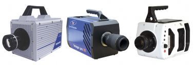
北京欧兰科技发展有限公司为您提供《全尺寸骑车人模型中气动阻力检测方案(CCD相机)》,该方案主要用于其他中气动阻力检测,参考标准--,《全尺寸骑车人模型中气动阻力检测方案(CCD相机)》用到的仪器有LaVision HighSpeedStar 高帧频相机、体视层析粒子成像测速系统(Tomo-PIV)、LaVision DaVis 智能成像软件平台
推荐专场
CCD相机/影像CCD
更多


相关方案
更多
该厂商其他方案
更多