


采用四台LaVision的16百万像素ImagerLX型相机构成体视层析PIV测量系统。从测量的单次层析PIV成像结果求得PIV的压力谱。
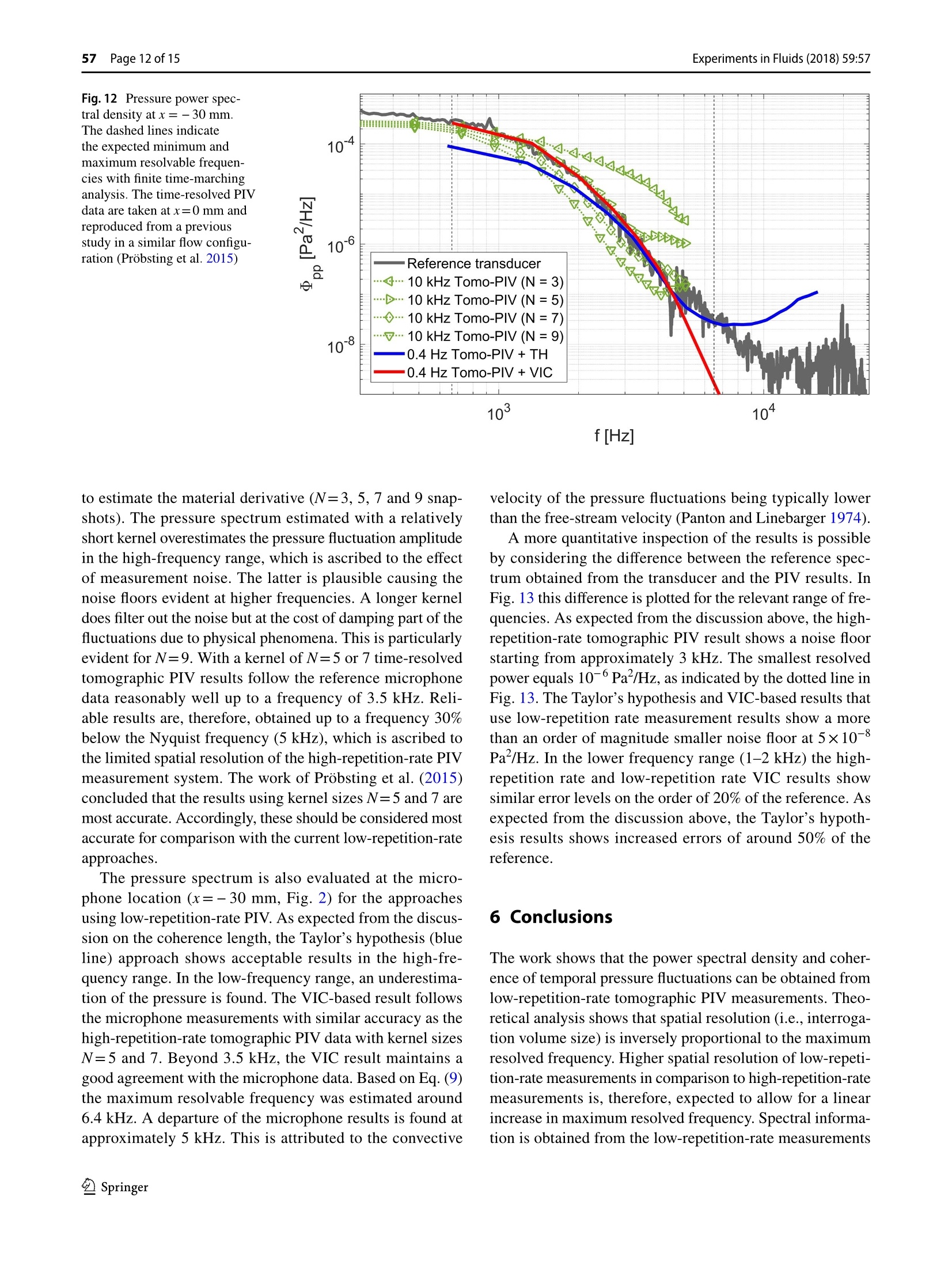
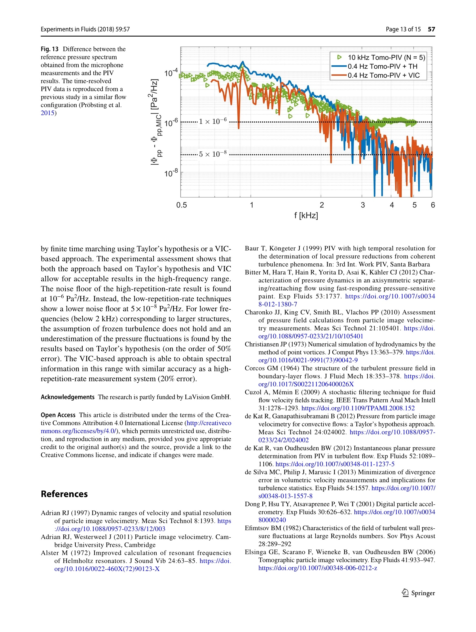
方案详情

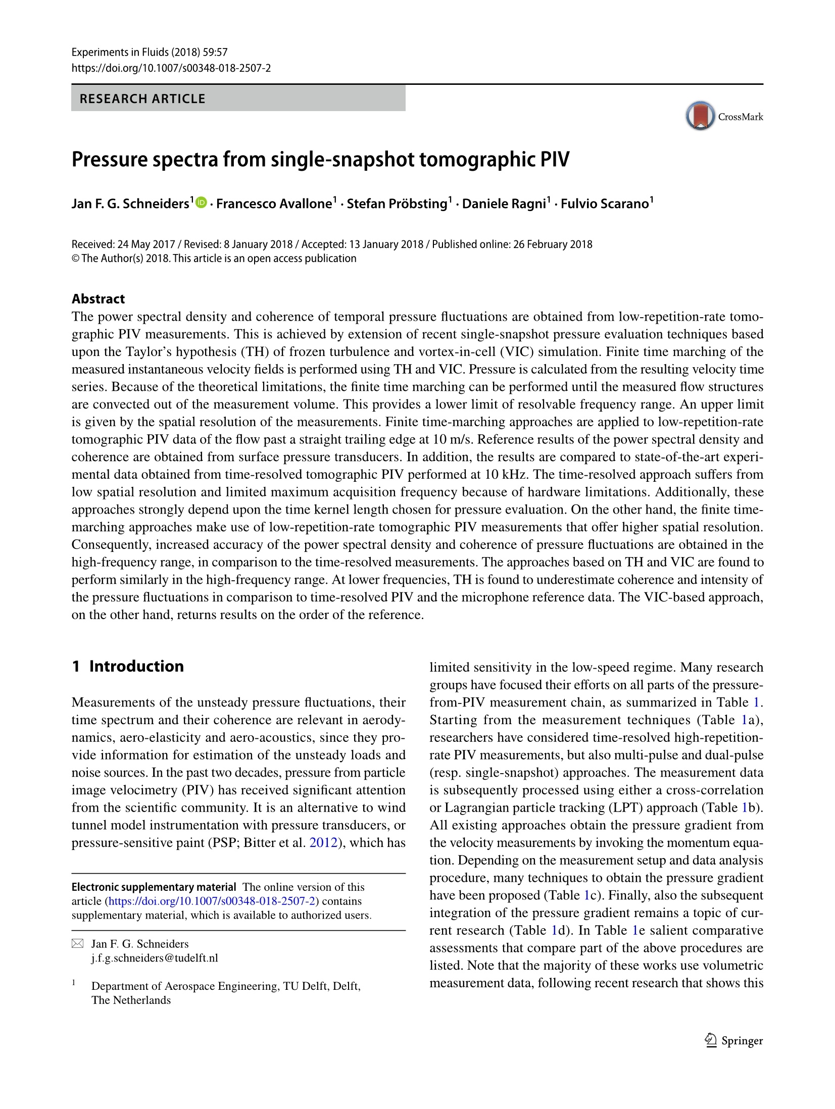
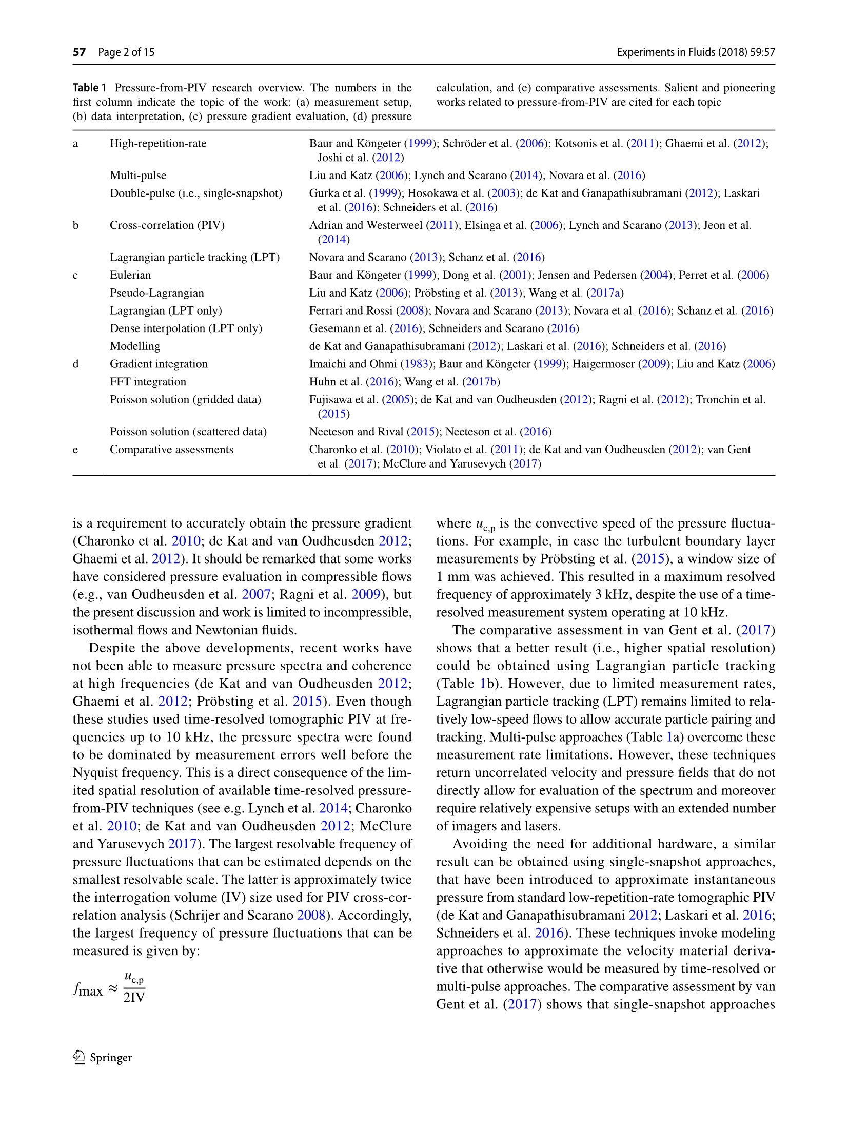
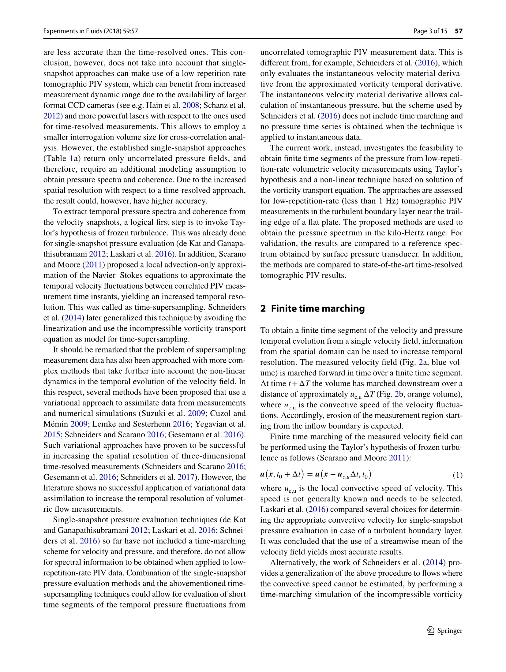
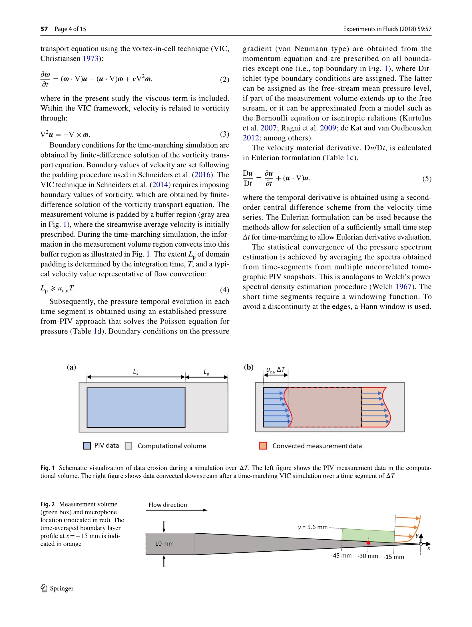
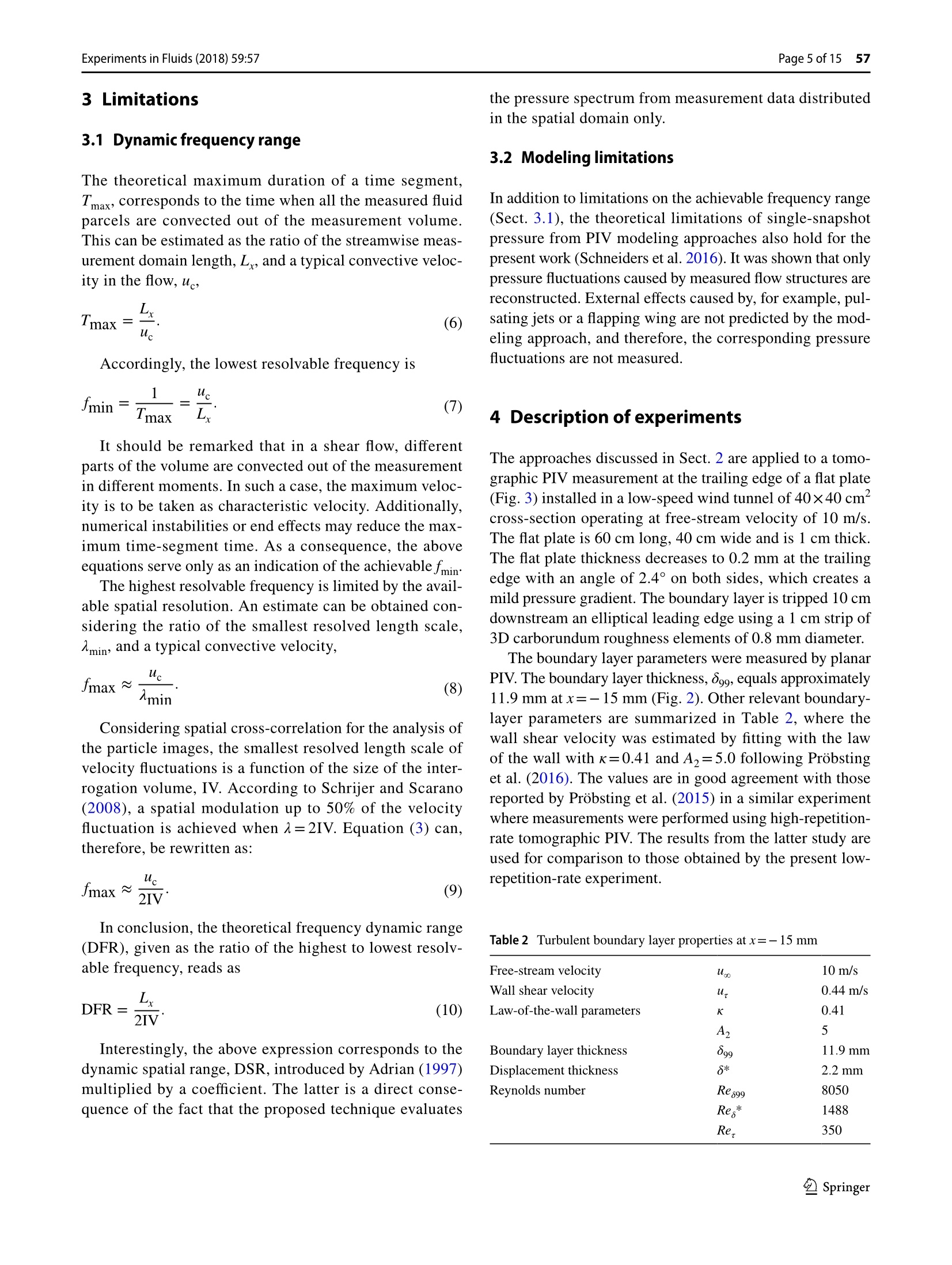
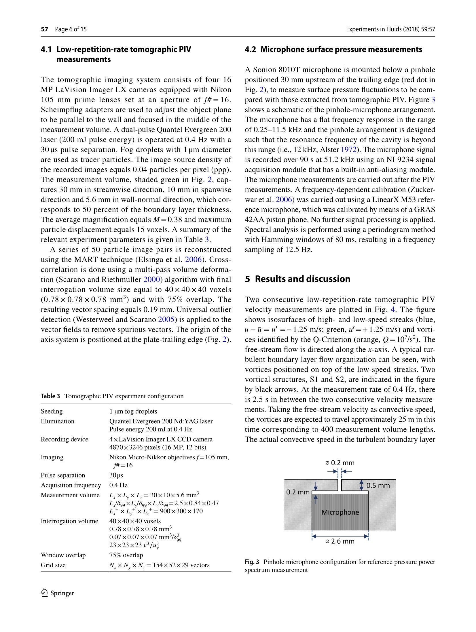
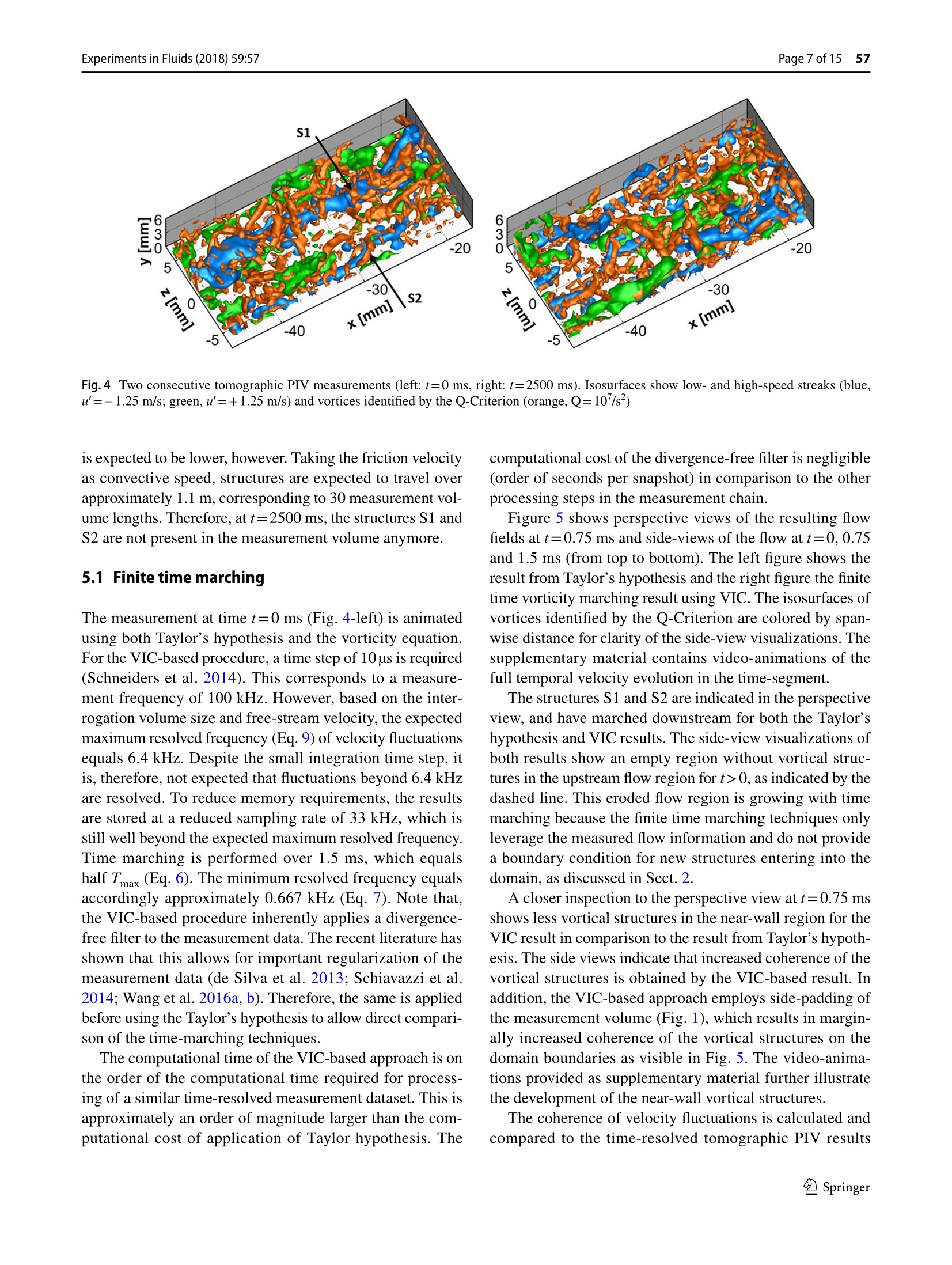
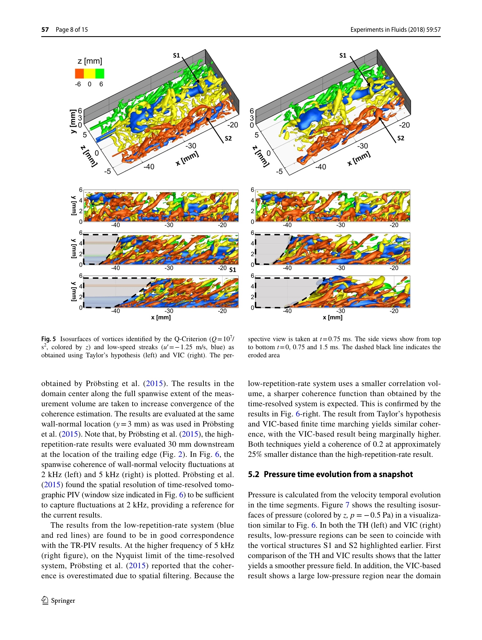
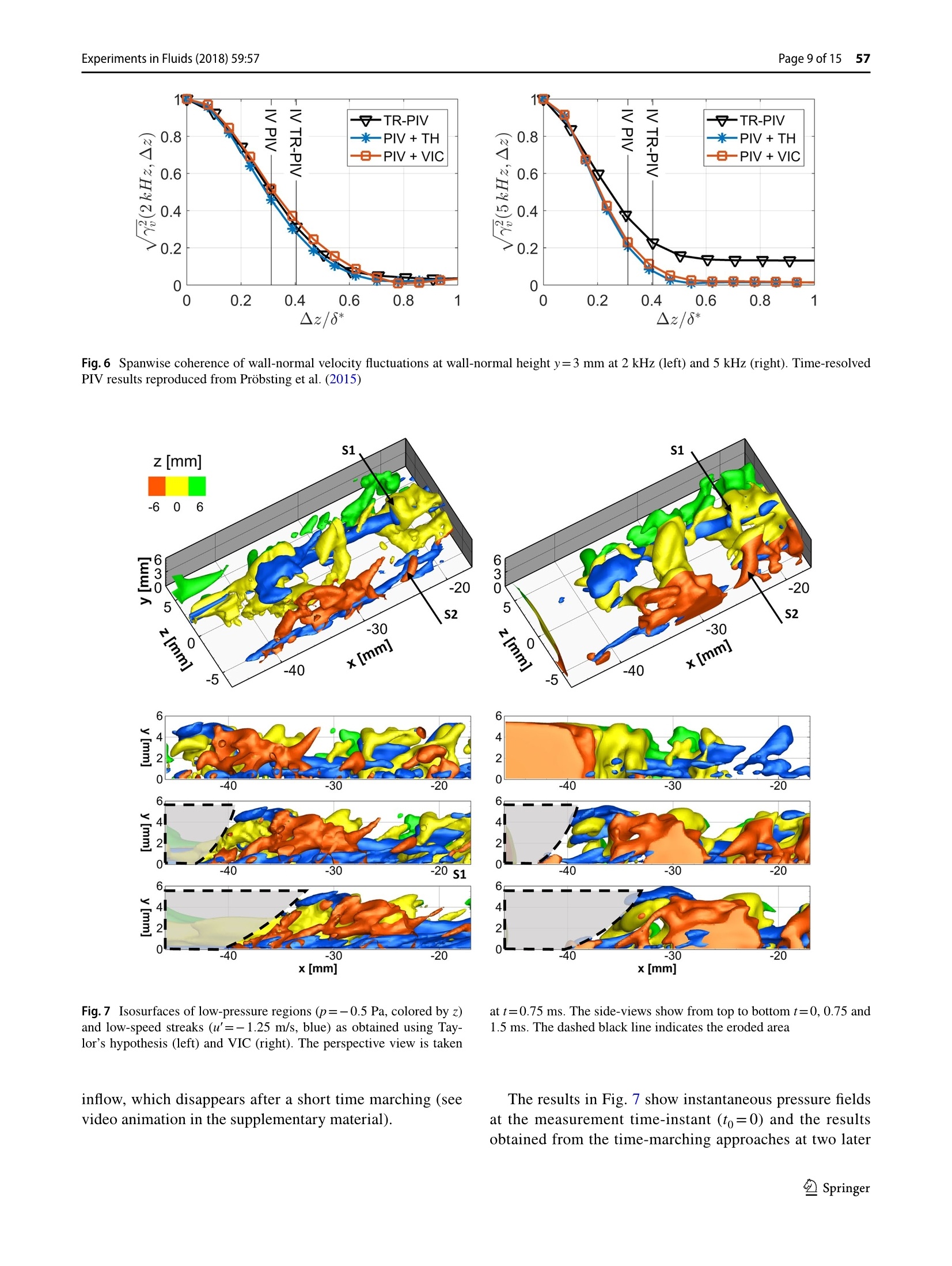
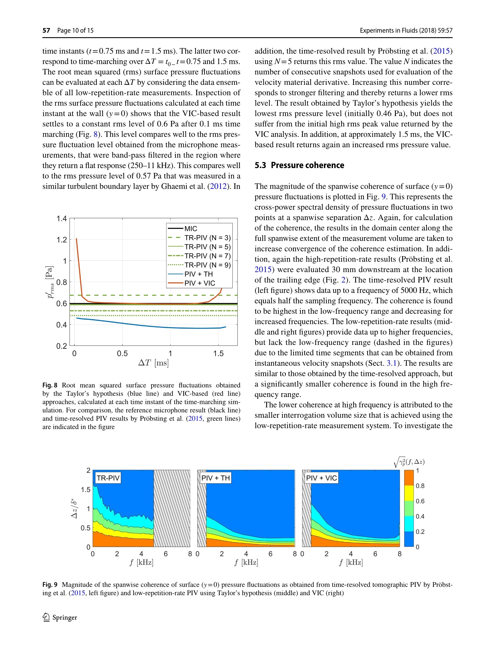
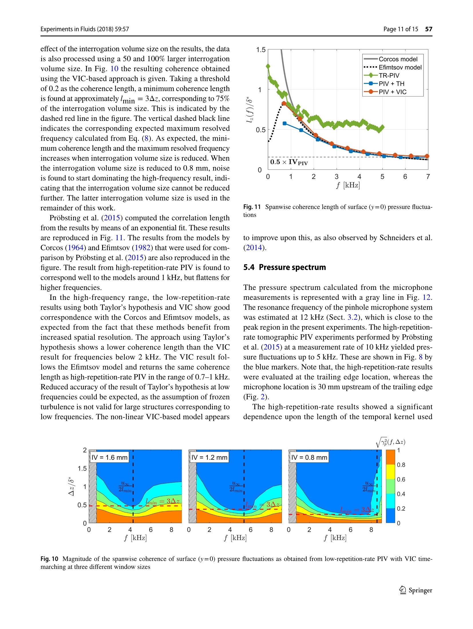
Experiments in Fluids (2018) 59:57https://doi.org/10.1007/s00348-018-2507-2 57 Page 2 of 15Experiments in Fluids (2018) 59:57 Pressure spectra from single-snapshot tomographic PIV Jan F. G. Schneider;sD. Francesco Avallonel·Stefan Probsting1·Daniele Ragnil·Fulvio Scarano Received: 24 May 2017 / Revised: 8 January 2018 / Accepted: 13 January 2018/Published online: 26 February 2018O The Author(s) 2018. This article is an open access publication Abstract The power spectral density and coherence of temporal pressure fluctuations are obtained from low-repetition-rate tomo-graphic PIV measurements. This is achieved by extension of recent single-snapshot pressure evaluation techniques basedupon the Taylor’s hypothesis (TH) of frozen turbulence and vortex-in-cell (VIC) simulation. Finite time marching of themeasured instantaneous velocity fields is performed using TH and VIC. Pressure is calculated from the resulting velocity timeseries. Because of the theoretical limitations, the finite time marching can be performed until the measured flow structuresare convected out of the measurement volume. This provides a lower limit of resolvable frequency range. An upper limitis given by the spatial resolution of the measurements. Finite time-marching approaches are applied to low-repetition-ratetomographic PIV data of the flow past a straight trailing edge at 10 m/s. Reference results of the power spectral density andcoherence are obtained from surface pressure transducers. In addition, the results are compared to state-of-the-art experi-mental data obtained from time-resolved tomographic PIV performed at 10 kHz. The time-resolved approach suffers fromlow spatial resolution and limited maximum acquisition frequency because of hardware limitations. Additionally, theseapproaches strongly depend upon the time kernel length chosen for pressure evaluation. On the other hand, the finite time-marching approaches make use of low-repetition-rate tomographic PIV measurements that offer higher spatial resolution.Consequently, increased accuracy of the power spectral density and coherence of pressure fluctuations are obtained in thehigh-frequency range, in comparison to the time-resolved measurements. The approaches based on TH and VIC are found toperform similarly in the high-frequency range. At lower frequencies, TH is found to underestimate coherence and intensity ofthe pressure fluctuations in comparison to time-resolved PIV and the microphone reference data. The VIC-based approach,on the other hand, returns results on the order of the reference. 1 Introduction Measurements of the unsteady pressure fluctuations, theirtime spectrum and their coherence are relevant in aerody-namics, aero-elasticity and aero-acoustics, since they pro-vide information for estimation of the unsteady loads andnoise sources. In the past two decades, pressure from particleimage velocimetry (PIV) has received significant attentionfrom the scientific community. It is an alternative to windtunnel model instrumentation with pressure transducers, orpressure-sensitive paint (PSP; Bitter et al. 2012), which has Electronic supplementary material The online version of thisarticle (https://doi.org/10.1007/s00348-018-2507-2) containssupplementary material, which is available to authorized users. 区Jan F. G. Schneiders j.f.g.schneiders @tudelft.nl Department of Aerospace Engineering, TU Delft, Delft,The Netherlands limited sensitivity in the low-speed regime. Many researchgroups have focused their efforts on all parts of the pressure-from-PIV measurement chain, as summarized in Table 1.Starting from the measurement techniques (Table 1a),researchers have considered time-resolved high-repetition-rate PIV measurements, but also multi-pulse and dual-pulse(resp. single-snapshot) approaches. The measurement datais subsequently processed using either a cross-correlationor Lagrangian particle tracking (LPT) approach (Table 1b).All existing approaches obtain the pressure gradient fromthe velocity measurements by invoking the momentum equa-tion. Depending on the measurement setup and data analysisprocedure, many techniques to obtain the pressure gradienthave been proposed (Table 1c). Finally, also the subsequentintegration of the pressure gradient remains a topic of cur-rent research (Table ld). In Table le salient comparativeassessments that compare part of the above procedures arelisted. Note that the majority of these works use volumetricmeasurement data, following recent research that shows this Table 1 Pressure-from-PIV research overview. The numbers in thefirst column indicate the topic of the work: (a) measurement setup, calculation, and (e) comparative assessments. Salient and pioneering. works related to pressure-from-PIV are cited for each topic a High-repetition-rate Baur and Kongeter (1999); Schroder et al. (2006);Kotsonis et al. (2011);Ghaemi et al. (2012); Joshi et al.(2012) Multi-pulse Liu and Katz (2006); Lynch and Scarano (2014); Novara et al.(2016) b Double-pulse (i.e., single-snapshot) Gurka et al.(1999); Hosokawa et al. (2003); de Kat and Ganapathisubramani (2012); Laskari et al.(2016); Schneiders et al.(2016) Cross-correlation (PIV) Adrian and Westerweel (2011); Elsinga et al. (2006); Lynch and Scarano (2013); Jeon et al. (2014) Lagrangian particle tracking (LPT) Novara and Scarano (2013); Schanz et al. (2016) Eulerian Baur and Kongeter (1999); Dong et al. (2001); Jensen and Pedersen (2004); Perret et al. (2006) Pseudo-Lagrangian Liu and Katz (2006); Probsting et al. (2013); Wang et al. (2017a) Lagrangian (LPT only) Ferrari and Rossi (2008); Novara and Scarano (2013); Novara et al. (2016); Schanz et al. (2016) d Dense interpolation (LPT only) Gesemann et al. (2016); Schneiders and Scarano (2016) Modelling de Kat and Ganapathisubramani (2012); Laskari et al. (2016); Schneiders et al. (2016) Gradient integration Imaichi and Ohmi (1983); Baur and Kongeter (1999); Haigermoser (2009);Liu and Katz (2006) FFT integration Huhn et al. (2016);Wang et al. (2017b) Poisson solution (gridded data) Fujisawa et al. (2005); de Kat and van Oudheusden (2012); Ragni et al. (2012); Tronchin et al. (2015) Poisson solution (scattered data) Neeteson and Rival (2015); Neeteson et al.(2016) e Comparative assessments Charonko et al. (2010); Violato et al. (2011); de Kat and van Oudheusden (2012); van Gent et al. (2017);McClure and Yarusevych (2017) is a requirement to accurately obtain the pressure gradient(Charonko et al. 2010; de Kat and van Oudheusden 2012;Ghaemi et al. 2012). It should be remarked that some workshave considered pressure evaluation in compressible flows(e.g., van Oudheusden et al. 2007; Ragni et al. 2009), butthe present discussion and work is limited to incompressible,isothermal flows and Newtonian fluids. Despite the above developments, recent works havenot been able to measure pressure spectra and coherenceat high frequencies (de Kat and van Oudheusden 2012;Ghaemi et al. 2012; Probsting et al. 2015). Even thoughthese studies used time-resolved tomographic PIV at fre-quencies up to 10 kHz, the pressure spectra were foundto be dominated by measurement errors well before theNyquist frequency. This is a direct consequence of the lim-ited spatial resolution of available time-resolved pressure-from-PIV techniques (see e.g. Lynch et al. 2014; Charonkoet al. 2010; de Kat and van Oudheusden 2012;McClureand Yarusevych 2017). The largest resolvable frequency ofpressure fluctuations that can be estimated depends on thesmallest resolvable scale. The latter is approximately twicethe interrogation volume (IV) size used for PIV cross-cor-relation analysis (Schrijer and Scarano 2008). Accordingly,the largest frequency of pressure fluctuations that can bemeasured is given by: where uc,p is the convective speed of the pressure fluctua-tions. For example, in case the turbulent boundary layermeasurements by Probsting et al. (2015), a window size of1 mm was achieved. This resulted in a maximum resolvedfrequency of approximately 3 kHz, despite the use of a time-resolved measurement system operating at 10 kHz The comparative assessment in van Gent et al. (2017)shows that a better result (i.e., higher spatial resolution)could be obtained using Lagrangian particle tracking(Table 1b). However, due to limited measurement rates,Lagrangian particle tracking (LPT) remains limited to rela-tively low-speed flows to allow accurate particle pairing andtracking. Multi-pulse approaches (Table 1a) overcome thesemeasurement rate limitations. However, these techniquesreturn uncorrelated velocity and pressure fields that do notdirectly allow for evaluation of the spectrum and moreoverrequire relatively expensive setups with an extended numberof imagers and lasers. Avoiding the need for additional hardware, a similarresult can be obtained using single-snapshot approaches,that have been introduced to approximate instantaneouspressure from standard low-repetition-rate tomographic PIV(de Kat and Ganapathisubramani 2012; Laskari et al. 2016;Schneiders et al. 2016). These techniques invoke modelingapproaches to approximate the velocity material deriva-tive that otherwise would be measured by time-resolved ormulti-pulse approaches. The comparative assessment by vanGent et al. (2017) shows that single-snapshot approaches are less accurate than the time-resolved ones. This con-clusion, however, does not take into account that single-snapshot approaches can make use of a low-repetition-ratetomographic PIV system, which can benefit from increasedmeasurement dynamic range due to the availability of largerformat CCD cameras (see e.g. Hain et al. 2008; Schanz et al.2012) and more powerful lasers with respect to the ones usedfor time-resolved measurements. This allows to employ asmaller interrogation volume size for cross-correlation anal-ysis. However, the established single-snapshot approaches(Table 1a) return only uncorrelated pressure fields, andtherefore, require an additional modeling assumption toobtain pressure spectra and coherence. Due to the increasedspatial resolution with respect to a time-resolved approach,the result could, however, have higher accuracy. To extract temporal pressure spectra and coherence fromthe velocity snapshots, a logical first step is to invoke Tay-lor’s hypothesis of frozen turbulence. This was already donefor single-snapshot pressure evaluation (de Kat and Ganapa-thisubramani 2012; Laskari et al. 2016). In addition, Scaranoand Moore (2011) proposed a local advection-only approxi-mation of the Navier-Stokes equations to approximate thetemporal velocity fluctuations between correlated PIV meas-urement time instants, yielding an increased temporal reso-lution. This was called as time-supersampling. Schneiderset al. (2014) later generalized this technique by avoiding thelinearization and use the incompressible vorticity transportequation as model for time-supersampling. It should be remarked that the problem of supersamplingmeasurement data has also been approached with more com-plex methods that take further into account the non-lineardynamics in the temporal evolution of the velocity field. Inthis respect, several methods have been proposed that use avariational approach to assimilate data from measurementsand numerical simulations (Suzuki et al. 2009; Cuzol andMemin 2009; Lemke and Sesterhenn 2016; Yegavian et al.2015; Schneiders and Scarano 2016; Gesemann et al. 2016).Such variational approaches have proven to be successfulin increasing the spatial resolution of three-dimensionaltime-resolved measurements (Schneiders and Scarano 2016;Gesemann et al.2016;Schneiders et al. 2017). However, theliterature shows no successful application of variational dataassimilation to increase the temporal resolution of volumet-ric flow measurements. Single-snapshot pressure evaluation techniques (de Katand Ganapathisubramani 2012; Laskari et al. 2016; Schnei-ders et al. 2016) so far have not included a time-marchingscheme for velocity and pressure, and therefore, do not allowfor spectral information to be obtained when applied to low-repetition-rate PIV data. Combination of the single-snapshotpressure evaluation methods and the abovementioned time-supersampling techniques could allow for evaluation of shorttime segments of the temporal pressure fluctuations from uncorrelated tomographic PIV measurement data. This isdifferent from, for example, Schneiders et al. (2016), whichonly evaluates the instantaneous velocity material deriva-tive from the approximated vorticity temporal derivative.The instantaneous velocity material derivative allows cal-culation of instantaneous pressure, but the scheme used bySchneiders et al. (2016) does not include time marching andno pressure time series is obtained when the technique isapplied to instantaneous data. The current work, instead, investigates the feasibility toobtain finite time segments of the pressure from low-repeti-tion-rate volumetric velocity measurements using Taylor’shypothesis and a non-linear technique based on solution ofthe vorticity transport equation. The approaches are assessedfor low-repetition-rate (less than 1 Hz) tomographic PIVmeasurements in the turbulent boundary layer near the trail-ing edge of a flat plate. The proposed methods are used toobtain the pressure spectrum in the kilo-Hertz range. Forvalidation, the results are compared to a reference spec-trum obtained by surface pressure transducer. In addition,the methods are compared to state-of-the-art time-resolvedtomographic PIV results. 2 Finite time marching To obtain a finite time segment of the velocity and pressuretemporal evolution from a single velocity field, informationfrom the spatial domain can be used to increase temporalresolution. The measured velocity field (Fig. 2a, blue vol-ume) is marched forward in time over a finite time segment.At time t+AT the volume has marched downstream over adistance of approximately uc.u AT (Fig. 2b, orange volume),where uc,u is the convective speed of the velocity fluctua-tions. Accordingly, erosion of the measurement region start-ing from the inflow boundary is expected. Finite time marching of the measured velocity field canbe performed using the Taylor’s hypothesis of frozen turbu-lence as follows (Scarano and Moore 2011): where ue,u is the local convective speed of velocity. Thisspeed is not generally known and needs to be selected.Laskari et al. (2016) compared several choices for determin-ing the appropriate convective velocity for single-snapshotpressure evaluation in case of a turbulent boundary layer.It was concluded that the use of a streamwise mean of thevelocity field yields most accurate results. Alternatively, the work of Schneiders et al. (2014) pro-vides a generalization of the above procedure to flows wherethe convective speed cannot be estimated, by performing atime-marching simulation of the incompressible vorticity transport equation using the vortex-in-cell technique (VIC,Christiansen 1973): where in the present study the viscous term is included.Within the VIC framework, velocity is related to vorticitythrough: Boundary conditions for the time-marching simulation areobtained by finite-difference solution of the vorticity trans-port equation. Boundary values of velocity are set followingthe padding procedure used in Schneiders et al. (2016). TheVIC technique in Schneiders et al.(2014) requires imposingboundary values of vorticity, which are obtained by finite-difference solution of the vorticity transport equation. Themeasurement volume is padded by a buffer region (gray areain Fig. 1), where the streamwise average velocity is initiallyprescribed. During the time-marching simulation, the infor-mation in the measurement volume region convects into thisbuffer region as illustrated in Fig. 1. The extent Lof domainpadding is determined by the integration time, T, and a typi-cal velocity value representative of flow convection: Subsequently, the pressure temporal evolution in eachtime segment is obtained using an established pressure-from-PIV approach that solves the Poisson equation forpressure (Table 1d). Boundary conditions on the pressure gradient (von Neumann type) are obtained from themomentum equation and are prescribed on all bounda-ries except one (i.e., top boundary in Fig. 1), where Dir-ichlet-type boundary conditions are assigned. The lattercan be assigned as the free-stream mean pressure level,if part of the measurement volume extends up to the freestream, or it can be approximated from a model such asthe Bernoulli equation or isentropic relations (Kurtuluset al. 2007; Ragni et al. 2009; de Kat and van Oudheusden2012; among others). The velocity material derivative,Du/Dt, is calculatedin Eulerian formulation (Table 1c). where the temporal derivative is obtained using a second-order central difference scheme from the velocity timeseries. The Eulerian formulation can be used because themethods allow for selection of a sufficiently small time stepAt for time-marching to allow Eulerian derivative evaluation. The statistical convergence of the pressure spectrumestimation is achieved by averaging the spectra obtainedfrom time-segments from multiple uncorrelated tomo-graphic PIV snapshots. This is analogous to Welch’s powerspectral density estimation procedure (Welch 1967). Theshort time segments require a windowing function. Toavoid a discontinuity at the edges, a Hann window is used. PIV data Computational volume Fig. 1 Schematic visualization of data erosion during a simulation over AT. The left figure shows the PIV measurement data in the computa-tional volume. The right figure shows data convected downstream after a time-marching VIC simulation over a time segment of AT Fig.2 Measurement volume(green box) and microphonelocation (indicated in red). Thetime-averaged boundary layerprofile at x=-15 mm is indi-cated in orange Flow direction 3 Limitations 3.1 Dynamic frequency range The theoretical maximum duration of a time segment,Tmax, corresponds to the time when all the measured fluidparcels are convected out of the measurement volume.This can be estimated as the ratio of the streamwise meas-urement domain length, Lx, and a typical convective veloc-ity in the flow,u, Accordingly, the lowest resolvable frequency is It should be remarked that in a shear flow, differentparts of the volume are convected out of the measurementin different moments. In such a case, the maximum veloc-ity is to be taken as characteristic velocity. Additionally,numerical instabilities or end effects may reduce the max-imum time-segment time. As a consequence, the aboveequations serve only as an indication of the achievable fi The highest resolvable frequency is limited by the avail-able spatial resolution. An estimate can be obtained con-sidering the ratio of the smallest resolved length scale,Amin, and a typical convective velocity, Considering spatial cross-correlation for the analysis ofthe particle images, the smallest resolved length scale ofvelocity fluctuations is a function of the size of the inter-rogation volume, IV. According to Schrijer and Scarano(2008), a spatial modulation up to 50% of the velocityfluctuation is achieved when A=2IV. Equation (3) can,therefore, be rewritten as: In conclusion,the theoretical frequency dynamic range(DFR), given as the ratio of the highest to lowest resolv-able frequency, reads as Interestingly, the above expression corresponds to thedynamic spatial range, DSR, introduced by Adrian (1997)multiplied by a coefficient. The latter is a direct conse-quence of the fact that the proposed technique evaluates the pressure spectrum from measurement data distributedin the spatial domain only. 3.2 Modeling limitations In addition to limitations on the achievable frequency range(Sect. 3.1),the theoretical limitations of single-snapshotpressure from PIV modeling approaches also hold for thepresent work (Schneiders et al.2016). It was shown that onlypressure fluctuations caused by measured flow structures arereconstructed. External effects caused by, for example, pul-sating jets or a flapping wing are not predicted by the mod-eling approach, and therefore, the corresponding pressurefluctuations are not measured. 4 Description of experiments The approaches discussed in Sect. 2 are applied to a tomo-graphic PIV measurement at the trailing edge of a flat plate(Fig.3) installed in a low-speed wind tunnel of 40×40 cmcross-section operating at free-stream velocity of 10 m/s.The flat plate is 60 cm long, 40 cm wide and is 1 cm thick.The flat plate thickness decreases to 0.2 mm at the trailingedge with an angle of 2.4° on both sides, which creates amild pressure gradient. The boundary layer is tripped 10 cmdownstream an elliptical leading edge using a 1 cm strip of3D carborundum roughness elements of 0.8 mm diameter. The boundary layer parameters were measured by planarPIV. The boundary layer thickness, 8g9, equals approximately11.9 mm at x=-15 mm (Fig.2). Other relevant boundary-layer parameters are summarized in Table 2, where thewall shear velocity was estimated by fitting with the lawof the wall with K=0.41 and A2=5.0 following Probstinget al. (2016). The values are in good agreement with thosereported by Probsting et al. (2015) in a similar experimentwhere measurements were performed using high-repetition-rate tomographic PIV. The results from the latter study areused for comparison to those obtained by the present low-repetition-rate experiment. Table 2 Turbulent boundary layer properties at x=-15 mm Free-stream velocity u. 10 m/s Wall shear velocity 0.44 m/s Law-of-the-wall parameters K 0.41 5 Boundary layer thickness 11.9 mm Displacement thickness 2.2 mm Reynolds number Res99 8050 Res 1488 Re 350 4.1 Low-repetition-rate tomographic PIVmeasurements The tomographic imaging system consists of four 16MP LaVision Imager LX cameras equipped with Nikon105 mm prime lenses set at an aperture of f#=16.Scheimpflug adapters are used to adjust the object planeto be parallel to the wall and focused in the middle of themeasurement volume. A dual-pulse Quantel Evergreen 2001aser (200 mJ pulse energy) is operated at 0.4 Hz with a30 us pulse separation. Fog droplets with 1 um diameterare used as tracer particles. The image source density ofthe recorded images equals 0.04 particles per pixel (ppp).The measurement volume, shaded green in Fig. 2, cap-tures 30 mm in streamwise direction, 10 mm in spanwisedirection and 5.6 mm in wall-normal direction, which cor-responds to 50 percent of the boundary layer thickness.The average magnification equals M=0.38 and maximumparticle displacement equals 15 voxels. A summary of therelevant experiment parameters is given in Table 3. A series of 50 particle image pairs is reconstructedusing the MART technique (Elsinga et al.2006). Cross-correlation is done using a multi-pass volume deforma-tion (Scarano and Riethmuller 2000) algorithm with finalinterrogation volume size equal to 40×40×40 voxels(0.78×0.78×0.78 mm’) and with 75% overlap. Theresulting vector spacing equals 0.19 mm. Universal outlierdetection (Westerweel and Scarano 2005) is applied to thevector fields to remove spurious vectors. The origin of theaxis system is positioned at the plate-trailing edge (Fig.2). Table 3 Tomographic PIV experiment configuration Seeding 1 um fog droplets Illumination Quantel Evergreen 200 Nd:YAG laser Pulse energy 200 mJ at 0.4 Hz Recording device 4×LaVision Imager LX CCD camera 4870×3246 pixels (16 MP, 12 bits) Imaging Nikon Micro-Nikkor objectives f=105 mm, f#=16 Pulse separation 30 us Acquisition frequency 0.4 Hz Measurement volume L×L,×L=30×10×5.6 mm’ L/899×L/899×L,/899=2.5×0.84×0.47 L+×L+×L+=900×300×170 Interrogation volume 40×40×40 voxels 0.78×0.78×0.78 mm’ 0.07×0.07×0.07mm’/83 23×23×23 v/u Window overlap 75% overlap Grid size N,×N,×N,=154×52×29 vectors 4.2 Microphone surface pressure measurements A Sonion 8010T microphone is mounted below a pinholepositioned 30 mm upstream of the trailing edge (red dot inFig. 2), to measure surface pressure fluctuations to be com-pared with those extracted from tomographic PIV. Figure 3shows a schematic of the pinhole-microphone arrangement.The microphone has a flat frequency response in the rangeof 0.25-11.5 kHz and the pinhole arrangement is designedsuch that the resonance frequency of the cavity is beyondthis range (i.e.,12 kHz, Alster 1972). The microphone signalis recorded over 90 s at 51.2 kHz using an NI 9234 signalacquisition module that has a built-in anti-aliasing module.The microphone measurements are carried out after the PIVmeasurements. A frequency-dependent calibration (Zucker-war et al. 2006) was carried out using a LinearX M53 refer-ence microphone, which was calibrated by means of a GRAS42AA piston phone. No further signal processing is applied.Spectral analysis is performed using a periodogram methodwith Hamming windows of 80 ms, resulting in a frequencysampling of 12.5 Hz. 5 Results and discussion Two consecutive low-repetition-rate tomographic PIVvelocity measurements are plotted in Fig. 4. The figureshows isosurfaces of high- and low-speed streaks (blue,u-u=u'=-1.25 m/s; green, u'=+1.25 m/s) and vorti-ces identified by the Q-Criterion (orange, Q=10’/s). Thefree-stream flow is directed along the x-axis. A typical tur-bulent boundary layer flow organization can be seen, withvortices positioned on top of the low-speed streaks. Twovortical structures, S1 and S2, are indicated in the figureby black arrows. At the measurement rate of 0.4 Hz, thereis 2.5 s in between the two consecutive velocity measure-ments. Taking the free-stream velocity as convective speed,the vortices are expected to travel approximately 25 m in thistime corresponding to 400 measurement volume lengths.The actual convective speed in the turbulent boundary layer Fig.3 Pinhole microphone configuration for reference pressure powerspectrum measurement Fig. 4 Two consecutive tomographic PIV measurements (left:t=0 ms, right:t=2500 ms). Isosurfaces show low- and high-speed streaks (blue,u'=-1.25 m/s; green, u'=+1.25 m/s) and vortices identified by the Q-Criterion (orange,Q=10’/s) is expected to be lower, however. Taking the friction velocityas convective speed, structures are expected to travel overapproximately 1.1 m, corresponding to 30 measurement vol-ume lengths. Therefore, at t=2500 ms, the structures S1 andS2 are not present in the measurement volume anymore. 5.1 Finite time marching The measurement at time t=0 ms (Fig. 4-left) is animatedusing both Taylor’s hypothesis and the vorticity equation.For the VIC-based procedure, a time step of 10 us is required(Schneiders et al. 2014). This corresponds to a measure-ment frequency of 100 kHz. However, based on the inter-rogation volume size and free-stream velocity, the expectedmaximum resolved frequency (Eq. 9) of velocity fluctuationsequals 6.4 kHz. Despite the small integration time step, itis, therefore, not expected that fluctuations beyond 6.4 kHzare resolved. To reduce memory requirements, the resultsare stored at a reduced sampling rate of 33 kHz, which isstill well beyond the expected maximum resolved frequency.Time marching is performed over 1.5 ms, which equalshalf Tmax (Eq.6). The minimum resolved frequency equalsaccordingly approximately 0.667 kHz (Eq. 7). Note that,the VIC-based procedure inherently applies a divergence-free filter to the measurement data. The recent literature hasshown that this allows for important regularization of themeasurement data (de Silva et al. 2013;Schiavazzi et al.2014; Wang et al.2016a, b).Therefore, the same is appliedbefore using the Taylor’s hypothesis to allow direct compari-. son of the time-marching techniques. The computational time of the VIC-based approach is onthe order of the computational time required for process-ing of a similar time-resolved measurement dataset. This isapproximately an order of magnitude larger than the com-putational cost of application of Taylor hypothesis. The computational cost of the divergence-free filter is negligible(order of seconds per snapshot) in comparison to the otherprocessing steps in the measurement chain Figure 5 shows perspective views of the resulting flowfields at t=0.75 ms and side-views of the flow at t=0, 0.75and 1.5 ms (from top to bottom). The left figure shows theresult from Taylor’s hypothesis and the right figure the finitetime vorticity marching result using VIC. The isosurfaces ofvortices identified by the Q-Criterion are colored by span-wise distance for clarity of the side-view visualizations. Thesupplementary material contains video-animations of thefull temporal velocity evolution in the time-segment. The structures S1 and S2 are indicated in the perspectiveview, and have marched downstream for both the Taylor’shypothesis and VIC results. The side-view visualizations ofboth results show an empty region without vortical struc-tures in the upstream flow region for t>0, as indicated by thedashed line. This eroded flow region is growing with timemarching because the finite time marching techniques onlyleverage the measured flow information and do not providea boundary condition for new structures entering into thedomain, as discussed in Sect. 2. A closer inspection to the perspective view at t=0.75 msshows less vortical structures in the near-wall region for theVIC result in comparison to the result from Taylor’s hypoth-esis. The side views indicate that increased coherence of thevortical structures is obtained by the VIC-based result. Inaddition, the VIC-based approach employs side-padding ofthe measurement volume (Fig. 1), which results in margin-ally increased coherence of the vortical structures on thedomain boundaries as visible in Fig.5. The video-anima-tions provided as supplementary material further illustratethe development of the near-wall vortical structures. The coherence of velocity fluctuations is calculated andcompared to the time-resolved tomographic PIV results Fig.5 Isosurfaces of vortices identified by the Q-Criterion (Q=10'/s, colored by z) and low-speed streaks (u'=-1.25 m/s, blue) asobtained using Taylor’s hypothesis (left) and VIC (right). The per- spective view is taken at t=0.75 ms. The side views show from topto bottom t=0,0.75 and 1.5 ms. The dashed black line indicates theeroded area obtained by Probsting et al. (2015). The results in thedomain center along the full spanwise extent of the meas-urement volume are taken to increase convergence of thecoherence estimation. The results are evaluated at the samewall-normal location (y=3 mm) as was used in Probstinget al. (2015). Note that, by Probsting et al.(2015), the high-repetition-rate results were evaluated 30 mm downstreamat the location of the trailing edge (Fig.2). In Fig. 6, thespanwise coherence of wall-normal velocity fluctuations at2 kHz (left) and 5 kHz (right) is plotted. Probsting et al.(2015) found the spatial resolution of time-resolved tomo-graphic PIV (window size indicated in Fig. 6) to be sufficientto capture fluctuations at 2 kHz, providing a reference forthe current results. low-repetition-rate system uses a smaller correlation vol-ume, a sharper coherence function than obtained by thetime-resolved system is expected. This is confirmed by theresults in Fig. 6-right. The result from Taylor’s hypothesisand VIC-based finite time marching yields similar coher-ence, with the VIC-based result being marginally higher.Both techniques yield a coherence of 0.2 at approximately25% smaller distance than the high-repetition-rate result. 5.2 Pressure time evolution from a snapshot The results from the low-repetition-rate system (blueand red lines) are found to be in good correspondencewith the TR-PIV results. At the higher frequency of 5 kHz(right figure), on the Nyquist limit of the time-resolvedsystem, Probsting et al.(2015) reported that the coher-ence is overestimated due to spatial filtering. Because the Pressure is calculated from the velocity temporal evolutionin the time segments. Figure 7 shows the resulting isosur-faces of pressure (colored by z, p=-0.5 Pa) in a visualiza-tion similar to Fig. 6. In both the TH (left) and VIC (right)results, low-pressure regions can be seen to coincide withthe vortical structures S1 and S2 highlighted earlier. Firstcomparison of the TH and VIC results shows that the latteryields a smoother pressure field. In addition, the VIC-basedresult shows a large low-pressure region near the domain Fig.6 Spanwise coherence of wall-normal velocity fluctuations at wall-normal height y=3 mm at 2 kHz (left) and 5 kHz (right). Time-resolvedPIV results reproduced from Probsting et al. (2015) -5 Fig. 7 Isosurfaces of low-pressure regions (p=-0.5 Pa, colored by z)and low-speed streaks (u'=-1.25 m/s, blue) as obtained using Tay-lor’s hypothesis (left) and VIC (right). The perspective view is taken at t=0.75 ms. The side-views show from top to bottom t=0, 0.75 and1.5 ms. The dashed black line indicates the eroded area inflow, which disappears after a short time marching (seevideo animation in the supplementary material). The results in Fig.7 show instantaneous pressure fieldsat the measurement time-instant (to=0) and the resultsobtained from the time-marching approaches at two later time instants (t=0.75 ms and t=1.5 ms). The latter two cor-respond to time-marching over AT=to_t=0.75 and 1.5 ms.The root mean squared (rms) surface pressure fluctuationscan be evaluated at each ▲T by considering the data ensem-ble of all low-repetition-rate measurements. Inspection ofthe rms surface pressure fluctuations calculated at each timeinstant at the wall (y=0) shows that the VIC-based resultsettles to a constant rms level of 0.6 Pa after 0.1 ms timemarching (Fig.8). This level compares well to the rms pres-sure fluctuation level obtained from the microphone meas-urements, that were band-pass filtered in the region wherethey return a flat response (250-11 kHz). This compares wellto the rms pressure level of 0.57 Pa that was measured in asimilar turbulent boundary layer by Ghaemi et al. (2012). In Fig.8 Root mean squared surface pressure fluctuations obtainedby the Taylor’s hypothesis (blue line) and VIC-based (red line)approaches, calculated at each time instant of the time-marching sim-ulation. For comparison, the reference microphone result (black line)and time-resolved PIV results by Probsting et al. (2015, green lines)are indicated in the figure addition, the time-resolved result by Probsting et al. (2015)using N=5 returns this rms value. The value N indicates thenumber of consecutive snapshots used for evaluation of thevelocity material derivative. Increasing this number corre-sponds to stronger filtering and thereby returns a lower rmslevel. The result obtained by Taylor’s hypothesis yields thelowest rms pressure level (initially 0.46 Pa), but does notsuffer from the initial high rms peak value returned by theVIC analysis. In addition, at approximately 1.5 ms, the VIC-based result returns again an increased rms pressure value. 5.3 Pressure coherence The magnitude of the spanwise coherence of surface (y=0)pressure fluctuations is plotted in Fig. 9. This represents thecross-power spectral density of pressure fluctuations in twopoints at a spanwise separation Az. Again, for calculationof the coherence, the results in the domain center along thefull spanwise extent of the measurement volume are taken toincrease convergence of the coherence estimation. In addi-tion, again the high-repetition-rate results (Probsting et al.2015) were evaluated 30 mm downstream at the locationof the trailing edge (Fig.2). The time-resolved PIV result(left figure) shows data up to a frequency of 5000 Hz, whichequals half the sampling frequency. The coherence is foundto be highest in the low-frequency range and decreasing forincreased frequencies. The low-repetition-rate results (mid-dle and right figures) provide data up to higher frequencies,but lack the low-frequency range (dashed in the figures)due to the limited time segments that can be obtained frominstantaneous velocity snapshots (Sect.3.1). The results aresimilar to those obtained by the time-resolved approach, buta significantly smaller coherence is found in the high fre-quency range. The lower coherence at high frequency is attributed to thesmaller interrogation volume size that is achieved using thelow-repetition-rate measurement system. To investigate the Fig.9 Magnitude of the spanwise coherence of surface (y=0) pressure fluctuations as obtained from time-resolved tomographic PIV by Probst-ing et al. (2015, left figure) and low-repetition-rate PIV using Taylor’s hypothesis (middle) and VIC (right) effect of the interrogation volume size on the results, the datais also processed using a 50 and 100% larger interrogationvolume size. In Fig. 10 the resulting coherence obtainedusing the VIC-based approach is given. Taking a thresholdof 0.2 as the coherence length, a minimum coherence lengthis found at approximately lmin =3Az, corresponding to 75%of the interrogation volume size. This is indicated by thedashed red line in the figure. The vertical dashed black lineindicates the corresponding expected maximum resolvedfrequency calculated from Eq. (8).As expected, the mini-mum coherence length and the maximum resolved frequencyincreases when interrogation volume size is reduced. Whenthe interrogation volume size is reduced to 0.8 mm, noiseis found to start dominating the high-frequency result, indi-cating that the interrogation volume size cannot be reducedfurther. The latter interrogation volume size is used in theremainder of this work. Probsting et al. (2015) computed the correlation lengthfrom the results by means of an exponential fit. These resultsare reproduced in Fig. 11. The results from the models byCorcos (1964) and Efimtsov (1982) that were used for com-parison by Probsting et al. (2015) are also reproduced in thefigure. The result from high-repetition-rate PIV is found tocorrespond well to the models around 1 kHz, but flattens forhigher frequencies. In the high-frequency range, the low-repetition-rateresults using both Taylor’s hypothesis and VIC show goodcorrespondence with the Corcos and Efimtsov models, asexpected from the fact that these methods benefit fromincreased spatial resolution. The approach using Taylor’shypothesis shows a lower coherence length than the VICresult for frequencies below 2 kHz. The VIC result fol-lows the Efimtsov model and returns the same coherencelength as high-repetition-rate PIV in the range of 0.7-1 kHz.Reduced accuracy of the result ofTaylor’s hypothesis at lowfrequencies could be expected, as the assumption of frozenturbulence is not valid for large structures corresponding tolow frequencies. The non-linear VIC-based model appears Fig. 11 Spanwise coherence length of surface (y=0) pressure fluctua-tions to improve upon this, as also observed by Schneiders et al.(2014). 5.4 Pressure spectrum The pressure spectrum calculated from the microphonemeasurements is represented with a gray line in Fig. 12.The resonance frequency of the pinhole microphone systemwas estimated at 12 kHz (Sect. 3.2), which is close to thepeak region in the present experiments. The high-repetition-rate tomographic PIV experiments performed by Probstinget al. (2015) at a measurement rate of 10 kHz yielded pres-sure fluctuations up to 5 kHz. These are shown in Fig. 8 bythe blue markers. Note that, the high-repetition-rate resultswere evaluated at the trailing edge location, whereas themicrophone location is 30 mm upstream of the trailing edge(Fig.2). The high-repetition-rate results showed a significantdependence upon the length of the temporal kernel used Fig.10 Magnitude of the spanwise coherence of surface (y=0) pressure fluctuations as obtained from low-repetition-rate PIV with VIC time-marching at three different window sizes Fig. 12 Pressure power spec-tral density at x=-30 mm.The dashed lines indicatethe expected minimum andmaximum resolvable frequen-cies with finite time-marchinganalysis. The time-resolved PIVdata are taken at x=0 mm andreproduced from a previousstudy in a similar flow configu-ration (Probsting et al. 2015) f[Hz] to estimate the material derivative (N=3, 5, 7 and 9 snap-shots). The pressure spectrum estimated with a relativelyshort kernel overestimates the pressure fluctuation amplitudein the high-frequency range,which is ascribed to the effectof measurement noise. The latter is plausible causing thenoise floors evident at higher frequencies. A longer kerneldoes filter out the noise but at the cost of damping part of thefluctuations due to physical phenomena. This is particularlyevident for N=9. With a kernel of N=5 or 7 time-resolvedtomographic PIV results follow the reference microphonedata reasonably well up to a frequency of 3.5 kHz.Reli-able results are, therefore, obtained up to a frequency 30%below the Nyquist frequency (5 kHz), which is ascribed tothe limited spatial resolution of the high-repetition-rate PIVmeasurement system. The work of Probstinget al. (2015)concluded that the results using kernel sizes N=5 and 7 aremost accurate. Accordingly, these should be considered mostaccurate for comparison with the current low-repetition-rateapproaches. The pressure spectrum is also evaluated at the micro-phone location (x=-30 mm, Fig. 2) for the approachesusing low-repetition-rate PIV. As expected from the discus-sion on the coherence length, the Taylor’s hypothesis (blueline) approach shows acceptable results in the high-fre-quency range. In the low-frequency range, an underestima-tion of the pressure is found. The VIC-based result followsthe microphone measurements with similar accuracy as thehigh-repetition-rate tomographic PIV data with kernel sizesN=5 and 7. Beyond 3.5 kHz, the VIC result maintains agood agreement with the microphone data. Based on Eq. (9)the maximum resolvable frequency was estimated around6.4 kHz. A departure of the microphone results is found atapproximately 5 kHz. This is attributed to the convective velocity of the pressure fluctuations being typically lower than the free-stream velocity (Panton and Linebarger 1974).A more quantitative inspection of the results is possibleby considering the difference between the reference spec-trum obtained from the transducer and the PIV results. InFig. 13 this difference is plotted for the relevant range of fre-quencies. As expected from the discussion above, the high-repetition-rate tomographic PIV result shows a noise floorstarting from approximately 3 kHz. The smallest resolvedpower equals 10-6Pa’/Hz, as indicated by the dotted line inFig. 13. The Taylor’s hypothesis and VIC-based results thatuse low-repetition rate measurement results show a morethan an order of magnitude smaller noise floor at 5×10-Pa²/Hz. In the lower frequency range (1-2 kHz) the high-repetition rate and low-repetition rate VIC results showsimilar error levels on the order of 20% of the reference. Asexpected from the discussion above, the Taylor’s hypoth-esis results shows increased errors of around 50% of thereference. 6 Conclusions The work shows that the power spectral density and coher-ence of temporal pressure fluctuations can be obtained fromlow-repetition-rate tomographic PIV measurements. Theo-retical analysis shows that spatial resolution (i.e., interroga-tion volume size) is inversely proportional to the maximumresolved frequency. Higher spatial resolution of low-repeti-tion-rate measurements in comparison to high-repetition-ratemeasurements is, therefore, expected to allow for a linearincrease in maximum resolved frequency. Spectral informa-tion is obtained from the low-repetition-rate measurements Fig. 13 Difference between thereference pressure spectrumobtained from the microphonemeasurements and the PIVresults. The time-resolvedPIV data is reproduced from aprevious study in a similar flowconfiguration (Probsting et al.2015) f [kHz] by finite time marching using Taylor’s hypothesis or a VIC-based approach. The experimental assessment shows thatboth the approach based on Taylor’s hypothesis and VICallow for acceptable results in the high-frequency range.The noise floor of the high-repetition-rate result is foundat 10-6Pa/Hz. Instead, the low-repetition-rate techniquesshow a lower noise floor at5×10-8 Pa’/Hz. For lower fre-quencies (below 2 kHz) corresponding to larger structures,the assumption of frozen turbulence does not hold and anunderestimation of the pressure fluctuations is found by theresults based on Taylor’s hypothesis (on the order of 50%error). The VIC-based approach is able to obtain spectralinformation in this range with similar accuracy as a high-repetition-rate measurement system (20% error). Acknowledgements The research is partly funded by LaVision GmbH. Open Access This article is distributed under the terms of the Crea-tive Commons Attribution 4.0 International License (http://creativecommons.org/licenses/by/4.0/), which permits unrestricted use, distribu-tion, and reproduction in any medium, provided you give appropriatecredit to the original author(s) and the source, provide a link to theCreative Commons license, and indicate if changes were made. References ( Adrian R J (1997) Dynamic ranges of velocity and spatial resolutionof particle image velocimetry. Meas Sci Technol 8:1393.h ttps : //doi .or g/10 . 1088/0957-0233/8 / 12/003 ) ( Adrian R J, W esterweel J(2011) Particle i m age velocimetry. Cam- bridge University Press, Cambridge ) ( Alster M ( 1972) I mproved c a lculation of resonant f requenciesof Helmholtz resonators. J Sound Vib 24:63-85. ht tps:/ / doi. org/10.1016/00 2 2-460X(72)90123-X ) Baur T, Kongeter J (1999) PIV with high temporal resolution forthe determination of local pressure reductions from coherentturbulence phenomena. In: 3rd Int. Work PIV, Santa Barbara ( Bitter M, Hara T, H ain R, Yorita D, Asai K, Kahler CJ ( 2 012) Char-acterization of pressure dynamics in an axisymmetric se p arat-ing/reattaching flow using fast-responding pressure-sensitivepaint. Exp F luids 5 3:1737. h t tps://doi.org /1 0.1007/s0034 8 -01 2 -1 3 80- 7 ) ( Charonko JJ, King CV, Smith BL, Vlachos PP (2010) Assessmentof pressure field calculations from particl e image velocime-try measurements. Meas Sci T e chnol 21:105401. htt ps:// d oi . org/10.1088/0957-0233/21/10/105401 ) ( Christiansen JP ( 1973) Numerical simulation of hydrodynamics by the method of point vortices. J Comput Phys 13:363-379. htt ps://doi.org/10.1016/0021-9991(73)90042-9 ) ( Corcos GM (1964) The structure of the turbulent pressure field in boundary-layer f lows.J Fluid Mech 1 8 :353-378. ht t ps://doi.org/10.1017/S00 2 211206400026X ) ( Cuzol A, Memin E ( 2009) A stochastic fi l tering technique for fluidflow velocity fields tracking. I EEE Trans Pattern Anal Mach Intell 31:1278-1 2 93. h t tp s://doi.org/10.1109/TPAMI.2008.152 ) ( de Kat R, Ganapathisubramani B (2012) Pressure from particle imagevelocimetry for convective flows: a Taylor’s hypothesis approach. Meas Sci Technol 24:024002. htt p s://doi.org/10.1088/0957- 0233/24/2/024002 ) ( de Kat R, van Oudheusden BW (2012) Instantaneous planar pressuredetermination f rom PIV i n turbulent f low. Exp Fluids 52:1089- 1106. https : //doi.org/10.1007/s00 3 48-01 1 -1237-5 ) ( de Silva MC, Philip J, Marusic I (2013) Minimization of divergenceerror in volumetric velocity measurements and implications for turbulence statistics. Exp Fluids 54:1557. h t tps://doi.org/10.1007/ s00348-013- 1 557-8 ) ( Dong P , Hsu TY, Atsavaprenee P, Wei T(2001) Digital particle accel-erometry. Exp F luids 30:626-632.h t tps://doi.org / 10 . 1007/s003480000240 ) ( Efimtsov BM (1982) Char a cteristics of the field of turbulent wall pres- sure fluctuations a t large Reynold s numbers. Sov Phys Acoust28:289-292 ) ( Elsinga GE, Scarano F, Wieneke B, van Oudheusden B W ( 2 006) Tomographic particle image velocimetry. Exp Fluids 41:933-947. h ttps: / /do i . or g / 10.1007/s00348-006-0212-z ) ( Ferrari S, Rossi L (2008) P article tracking velocimetry and acceler- ometry (PTVA) measurements applied to quasi-two-dimensional multi-scale flows. Exp Fluids 44:873-886. ht tps: / /doi.org/ 10 .1 0 07/ s00348-007-04 4 3- 7 ) Fujisawa N, Tanahashi S, Srinavas K (2005) Evaluation of pressure fieldand fluid forces on a circular cylinder with and without rotationaloscillation using velocity data from PIV measurement. Meas SciTechnol 16:989-996. https://doi.org/10.1088/0957-0233/16/4/011 Gesemann S, Huhn F, Schanz D, Schroder A (2016) From noisy par-ticle tracks to velocity, acceleration and pressure fields usingB-splines and penalties. In: 18th Int. Symp. on Applications ofLaser and Imaging Techniques to Fluid Mechanics. Lisbon, Por-tugal, 4-7 July 2016 ( Ghaemi S, Ragni D, Scarano F (2012) PIV-based pressure fluctuations in the turbulent boundary layer. Exp Fluids 5 3:1823-1840. ht t ps : //do i .org / 10 . 1007 / s00348-012-1 3 9 1-4 ) ( Gurka R, Liberzon A , H e fetz D, R u binstein D, Shavit U (1999) Com-putation of pressure distribution using PIV v elocity data. In: 3rdInt. Workshop on Particle Image Velocimetry, Santa B a rbara, pp 671 - 676 ) ( Haigermoser C (2009) A p plication o f an acoustic a nalogy to P IV data f rom rectangular cavity flows. Exp Fluids 47:145-157. h ttps: / /d o i.org/10.1007/s00348-009-0642 - 5 ) ( Hain R, K ahler CJ, Michaelis D (2008) Tomographic and time resolvedPIV measurements on a finite cylinder on a f l at plate. Exp Fluids 45:715-724. h ttps://doi.org/10.1007/s00 3 48-008-0553-x ) ( Hosokawa S , Moriyama S, Tomiyama A , Takada N (2003) PIVmeasurement of p r essure distributions a bout s ingle b ubbles. JNucl S ci T echnol 40:754-762. h t tps://doi.or g/1 0.1080/1 8 811 248.2003 . 97154 1 6 ) ( Huhn F, S chanz D, Gesemann S, Schroder A (2016) FFT integration of i nstantaneous 3D pressure gradient fields measured by Lagrangian particle tracking in turbulent flows. Exp Fluids 57:151. ht t ps:// d oi.org/10.1007/s00348-016-2236-3 ) ( Imaichi K,Ohmi K ( 1 9 83) Numerical pro c essing of flow-visualization pictures—measurement of two-dimensional fl o w. J F l uid Mech 129:283-311.h ttps://doi. or g/10.1017/S002 21 12083000774 ) ( Jensen A , P edersen GK (2004) Optimization of acceleration measure- ments using PIV. Meas S c i Technol 1 5 :2275-2283. htt ps://doi. org/10.1088/0957-0233/15/1 1 /01 3 ) ( Jeon YJ, Chatellier L , D avid L (2014) Fluid trajectory evaluation b a sed on an e nsemble-averaged cross-correlation in ti m e-resolved PIV . Exp Fluids 55:1766. h ttps : //doi.org/10 . 100 7 /s00348-014-17 6 6-9 ) ( Joshi P , Liu X, Katz J (2012) Modification of turbulence in boundarylayers by mean and fluctuating pressure gradien t s FEDSM2012- 72280: A SME 2012 Fl u ids Engineering Summer Meeting, Puerto Rico ) ( Kotsonis M, Ghaemi S, Veldhuis L, S carano F (2011) M easurement of the body force field of plasma actuators. J Phys D Appl P h ys44:045204. h t tp s://doi.o r g / 10.1088/0022-3727/44/4/045204 ) ( Kurtulus DF, Scarano F, David L (2007) Unsteady aerodynamic forcesestimation on a square c ylinder by TR-PIV. Exp Fluids 42:185- 196. https : //doi.org/1 0 .1007/s00348-006-0 2 28-4 ) ( Laskari A, de Kat R , Ganapathisubramani B (2016) Fu l l-field pres- sure from s napshot and time-resolved volumetric PIV. Exp Fluids 57:44. https://doi.org/10.1007/s00348-016-212 9 -5 ) ( Lemke M, Sesterhenn J (2016) A d joint-based pressure determinationfrom PIV data in compressible flows—validation and assessmentbased o n synthetic data. Eur J Mech B /Fluids 58:29-38. h ttps: / / doi.o rg /10.1016/j.eurome ch flu.2016.03.006 ) ( Liu X, K atz J (2006) I nstantaneous p ressure and material accelera-tion measurements using a f our-exposure PIV system. Exp Fluids 41:227.h ttps: / /doi.o rg /10.1007/s00348-006-015 2 -7 ) ( Lynch K , Scarano F (2013) A high-order time-accurate in t errogation method for time-resolved PIV. Meas Sci Technol 24:035305. ht t ps : //doi.org/1 0 .1088/0957-0233/24/3/035305 ) ( Lynch K P , S c arano F (2014) Material acceleration estimation byfour-pulse tomo-PIV. Meas Sci Technol 25:084005. htt p s :// do i. o rg / 1 0.1088/0957-0233/25/8/084005 ) ( Lynch KP, Probsting S, Scarano F (2014) Temporal resolution oftime-resolved tomographic PI V in t urbulent boundary layers.In: Proceedings of the 17th international symposium on applica-tions of laser techniques to fluid mechanics, Lisbon, Portugal, 7-10 July,2014 ) ( McClure J, Y arusevych S (2017) Instantaneous PIV/PTV-based pres-sure gradient estimation: a framework for error analysis and correction. E xp F l uids 58:92. ht tps://doi. o rg/ 10 .1 00 7/s0034 ) ( Neeteson N J , R i val D E (2015) Pressure-field extraction on unstruc-tured flow data using a Voronoi tessellation-based networkingalgorithm: a proof-of-principle study. Exp Fluids 56:44. htt p s : //do i. org/10 . 1007/s00348-015 - 19 1 1 - 0 ) ( Neeteson N J, B hattacharya S , Rival DE, Michaelis D, Schanz D,Schroder A (2016) P r essure-field extraction f rom Lagrangian 丁 1 . flow measurements: f irst experiences with 4D-PTV data. Exp Fluids 57:102.h ttps://do i .org/10.100 7 /s00348-016-217 0 -4 ) ( N ovara M, Scarano F ( 2013) A particle-tracking approach for accu-rate material derivative measurements with tomographic PIV. Exp Fluids 54:1584. h ttps://doi.o rg /10.1007/s0 0 348-013-1584-5 ) ( Novara M, Schanz D, Reuther N, Kahler C J , Schroder A ( 2 016)Lagrangian 3 D particle tracking i n high-speed flows: shake-the-box f o r multi-pulse systems. Exp Flu i ds 57:128. http s ://doi.org/ 1 0. 1 007/s00 3 48-016-2216-7 ) ( Panton R L, Linebarger JH (1974) Wall pressure spectra calculations for equilibrium boundary l ayers. J Fluid Mech 65:261-287. https : //do i . or g/1 0 . 10 1 7/S002211 2 07 4 001388 ) ( Perret L, Braud P, Fourment C, David L,Delville J (2006) 3-Compo-nent acceleration field measurement by dual-time stereoscopicparticle image velocimetry. Exp Fluids 40:813-824. htt ps://doi. o rg /10.1007/s00348-006-0121- 1 ) ( Probsting S, Scarano F, Bernardini M, Pirozzoli S (20 1 3) On the esti-mation o f wall pressure coherence using time-resolved tomo- graphic PIV. Exp Fluids 54:15 6 7. ht t ps://doi.org/1 0. 1007/s0034 8-013-1 5 67-6 ) ( Probsting S, Tuinstra M, Scarano F(2015)Trailing edge noise esti- mation by tomographic particle image velocimetry. J Sound Vib346:117-138. h t tps:/ / doi.org / 10.1016/j .js v.2015 . 02.018 ) ( Probsting S, Schneiders JFG, Avallone F, Ragni D, Scarano F (2016) Trailing-edge noise diagnostics with low-repetition-rate PIV. 22n d AIAA/CEAS Aeroacoustics Conference, Aeroacoustics Confer- ences, (AIAA 2016-3023).ht tps://doi.org/10.2514/6.2016 - 3023 ) ( Ragni D, Ashok A, van Oudheusden BW, Scarano F (2009) Surfacepressure and aerodynamic loads determination of a transonicairfoil based on particle image velocimetry . Meas Sci Technol 20:074005. h ttps://do i .org/1 0 .1088/095 7 -0 2 33/20/7/0 7 4005 ) ( Ragni D , van Oudheusden B W , Scarano F (2012) 3 D pressure imag-ing of a propeller blade tip region by phase-locked stereoscopic PIV.Exp Fluids 52:463-477 ) ( Scarano F, Moore P (2011) A n advection-based model to increase thetemporal resolution o f PIV time series. Exp F luids 52:919-933. h t t ps://doi.org/10.1007/s00348-011-11 5 8-3 ) ( Scarano F, Riethmuller M L (2000) Advances in iter a tive multigrid P IV image processing. E xp Fluids 29:S051-S060. h t t ps://doi . o rg / 1 0 .1 00 7 /s0034800 7 000 7 ) ( Schanz D, Schroder A , H e ine B, Dierksheide U ( 2 0 12) Flow struc- ture identification in a high-resolution tomographic PIV dataset of the flow behind a backward facing step. I n:Proceedingsof the 16th international symposium on a p plications of lasertechniques to fluid mechanics, Lisbon, Portugal, 9-12 July 2012 ) ( Schanz D, Gesemann S , Schroder A (2016) Shake-The-Box: Lagran-gian particle tracking at high particle image densities. Exp Flu- ids 57:70. https://doi.org / 10 . 1007/s00348-016-2157-1 ) ( Schiavazzi D, Coletti F, Iaccarino G, Eato n JK (2014) A matching pursuit approach to s olenoidal f iltering of three-dimensional velocity measurements. J Comput P h ys 2 6 3:206-221.htt ps:// doi.org/1 0 .101 6 /j. jcp. 2013.12.049 ) ( Schneiders JFG, Scarano F (2016) Dense velocity r e construction fromtomographic ptv with material derivatives. Exp Fluids 57:139. https://doi.org/10.1007/s003 4 8-016-2225-6 ) ( Schneiders JFG, Dwight RP, Scarano F (2014) Time-supersampling of 3D-PIV measurements with vortex-in-cell simulation. Exp Fluids 5 5:1692. h ttps://do i .o rg /10.1007/s00348- 0 14-1 69 2-x ) ( Schneiders JFG, P robsting S, Dwight R P, v an O udheusden BW,Scarano F (2016) P ressure estimation from single-snapshot tomo-graphic PIV i n a turbulent boundary layer. Exp Fluids 57:53. ht t ps : //do i .org / 10.1007/s00 3 48-016-2 1 3 3- 9 ) ( Schneiders JFG, Scarano F, Elsinga G(2017)Resolving vorticity anddissipation in a turbulent boundary l ayer by tomographic P T V and VIC+. Exp Fluids 5 8 :27. h ttps: / /doi.org/10.1007/s0034 8 -017-2318 - x ) ( Schrijer F FJ, S carano F (2008) Effect of predictor-corrector filteringon t he stability and s patial resolution of i terative PIV interro- gation. Exp F luids 45:927-941. h ttps://d o i.or g /10. 1 007/s0034 8 -008-0511 - 7 ) ( Schroder A, Herr M, Lauke T, Dierksheide U (2006) A study ontrailing-edge noise sources using h igh-speed particle i mage velocimetry. Notes N umer Fluid Mech 92:373-380. http s :// do i.org/10.1007/978-3-540-33287-9_ 4 6 ) ( Suzuki T, Ji H, Yamamoto F (2009) Unsteady PTV velocity field pastan a irfoil solved with DNS: Part 1. Algorithm of h y brid simula-tion and hybrid velocity field at Re~ 103. Exp Fluids 47:957-976. https://do i .org / 1 0 .1007/s00348 - 009-0691-9 ) ( Tronchin T, David L, Farcy A (2015) Ev a luation of pressure field and f luid forces for 3D flow around flapping wing. Exp Fluids 56:1. ht t ps : //d o i.or g /10.10 0 7/s00 3 48-014-1870-x ) ( van Oudheusden BW (2013) PIV-Based pr e ssure m e asurement.Meas Sci Technol 2 4 :032001. ht t ps://doi.org/10.1088/0957- 0233/24/3/032001 ) ( van Oudheusden BW, Scarano F, R oosenboom EW, Casimiri EW, Souverein L J (2007) Evaluation of integral forces an d pressure fields from planar velocimetry data for incompressible and com-pressible flows. Exp Fluids 43:1 5 3. h ttp s ://doi. o rg /10 .1007/s 0 034 8 -007-0261 - y ) ( van Gent P, Michaelis D, van Oudheusden BW, Weiss P-E, de Kat R, Laskari A, Jeon YJ, David L, Schanz D, Huhn F , GesemannS, Novara M, McPhaden C , Neeteson N, Rival D , S chneidersJFG, Schrijer F (201 7 ) Comparative assessment of pressure field reconstructions from particle image velocimetry measurements and Lagrangian particle t r acking. Exp Fluids 58 : 33. ht t ps://doi. o rg /10.1007/s00348-01 7 - 2 3 2 4-z ) ( Violato D , Moore P, Scarano F (2011) Lagrangian and Eulerian pres- sure field evaluation of rod-airfoil flow from time-resolved tomo- graphic P IV. E xp Fluids 50:1057-1070. ht tps: / / doi. o rg/ 10 .1007/ s00348-010-1011-0 ) ( Wang C, Gao Q, Wang H, Wei R, Li T, Wang J (2016a) Divergence- free smoothing f o r volumetric PIV data. Exp Fluids 57 : 15. ht t ps://doi. or g / 10.1007/s00348-015-2097-1 ) ( Wang Z, Gao Q, Wang C, W e i R , W a ng J ( 2016b) An irrotation cor-rection on p ressure gradient and orthogonal-path in t egration for P IV-based pressure reconstruction. Ex p Fluids 57:104.http s ://doi. or g /10.1007/s00348-016-2189-6 ) ( Wang Z, Gao Q, Pan C, Feng L, Wa n g J (20 1 7a) Imaginary particletracking accelerometry based on time-resolved velocity fields. Exp Fluids 58:113. https://doi.org/10.1007/s00348-01 7 -2394-y ) ( Wang CY, Gao Q, Wei R J , Li T , Wang JJ (2017b) Spectral decomposi-tion-based fast pressure integration algorithm. Exp Fluids 58:84. h t t ps://doi.org/10.1007/s00348-017-2368-0 ) ( Welch P D (1 9 6 7) The u se of f ast Fourier transform for the estimation of power spectra: a method based on t i me averaging over short, modified periodograms. IEEE Trans Audio E lectroacoust AU 1 5:70-73. h ttps://do i .o rg /10 . 1109/TAU. 19 67.1 1 61901 ) ( Westerweel J , Scarano F (2005) Un i versal ou t lier detection for P I V data. Exp F luids 3 9:1096-1100. h t tps://doi.org / 10. 1 007/s0034 8-005-0016 - 6 ) ( Yegavian R, L eclaire B, Champagnat F, Marquet O ( 2015) Perfor-mance assessment of PIV super-resolution w i th adjoint-based dataassimilation. In: Proceedings of the 11th Int. Symp. on PIV, SantaBarbara, CA, US, 14-16 Sep 2015 ) ( Zuckerwar AJ, H e rring GC, El b ing BR (2006) Calibration of t hepressure sensitivity of microphones by a free-field met h od at fre-quencies up to 80 kHz. J Acoust Soc Am 119 : 320. http s://doi.org/10.1121/ 1. 2141360 ) Springer The power spectral density and coherence of temporal pressure fluctuations are obtained from low-repetition-rate tomographic PIV measurements. This is achieved by extension of recent single-snapshot pressure evaluation techniques based upon the Taylor’s hypothesis (TH) of frozen turbulence and vortex-in-cell (VIC) simulation. Finite time marching of themeasured instantaneous velocity fields is performed using TH and VIC. Pressure is calculated from the resulting velocity time series. Because of the theoretical limitations, the finite time marching can be performed until the measured flow structures are convected out of the measurement volume. This provides a lower limit of resolvable frequency range. An upper limit is given by the spatial resolution of the measurements. Finite time-marching approaches are applied to low-repetition-rate tomographic PIV data of the flow past a straight trailing edge at 10 m/s. Reference results of the power spectral density and coherence are obtained from surface pressure transducers. In addition, the results are compared to state-of-the-art experimental data obtained from time-resolved tomographic PIV performed at 10 kHz. The time-resolved approach suffers from low spatial resolution and limited maximum acquisition frequency because of hardware limitations. Additionally, these approaches strongly depend upon the time kernel length chosen for pressure evaluation. On the other hand, the finite timemarching approaches make use of low-repetition-rate tomographic PIV measurements that offer higher spatial resolution. Consequently, increased accuracy of the power spectral density and coherence of pressure fluctuations are obtained in the high-frequency range, in comparison to the time-resolved measurements. The approaches based on TH and VIC are found to perform similarly in the high-frequency range. At lower frequencies, TH is found to underestimate coherence and intensity of the pressure fluctuations in comparison to time-resolved PIV and the microphone reference data. The VIC-based approach, on the other hand, returns results on the order of the reference.
确定

还剩13页未读,是否继续阅读?

产品配置单


北京欧兰科技发展有限公司为您提供《流体中压力场检测方案(CCD相机)》,该方案主要用于其他中压力场检测,参考标准--,《流体中压力场检测方案(CCD相机)》用到的仪器有Imager LX PIV相机、体视层析粒子成像测速系统(Tomo-PIV)、LaVision DaVis 智能成像软件平台
推荐专场


相关方案
更多
该厂商其他方案
更多