二维剪切流中速度矢量场检测方案(CCD相机)

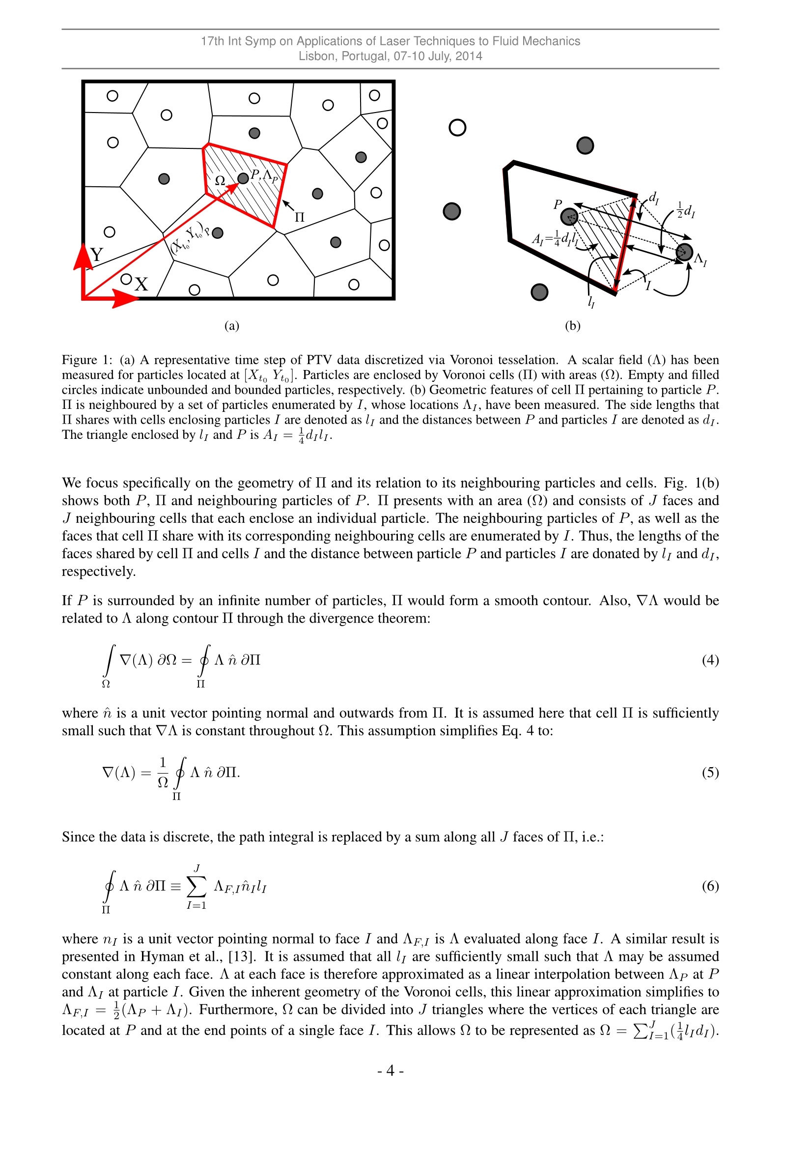
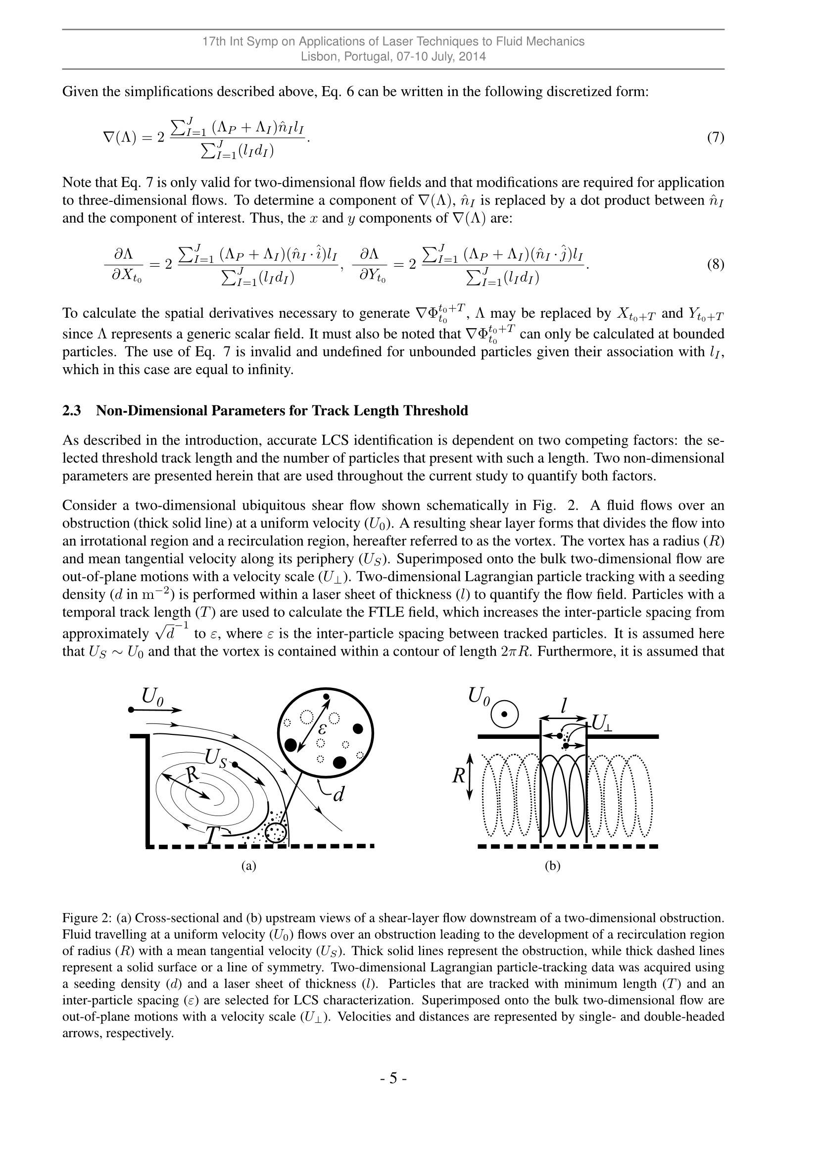
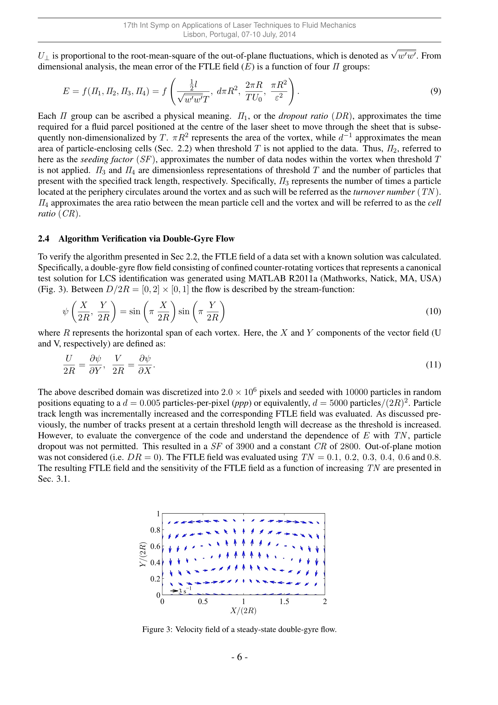
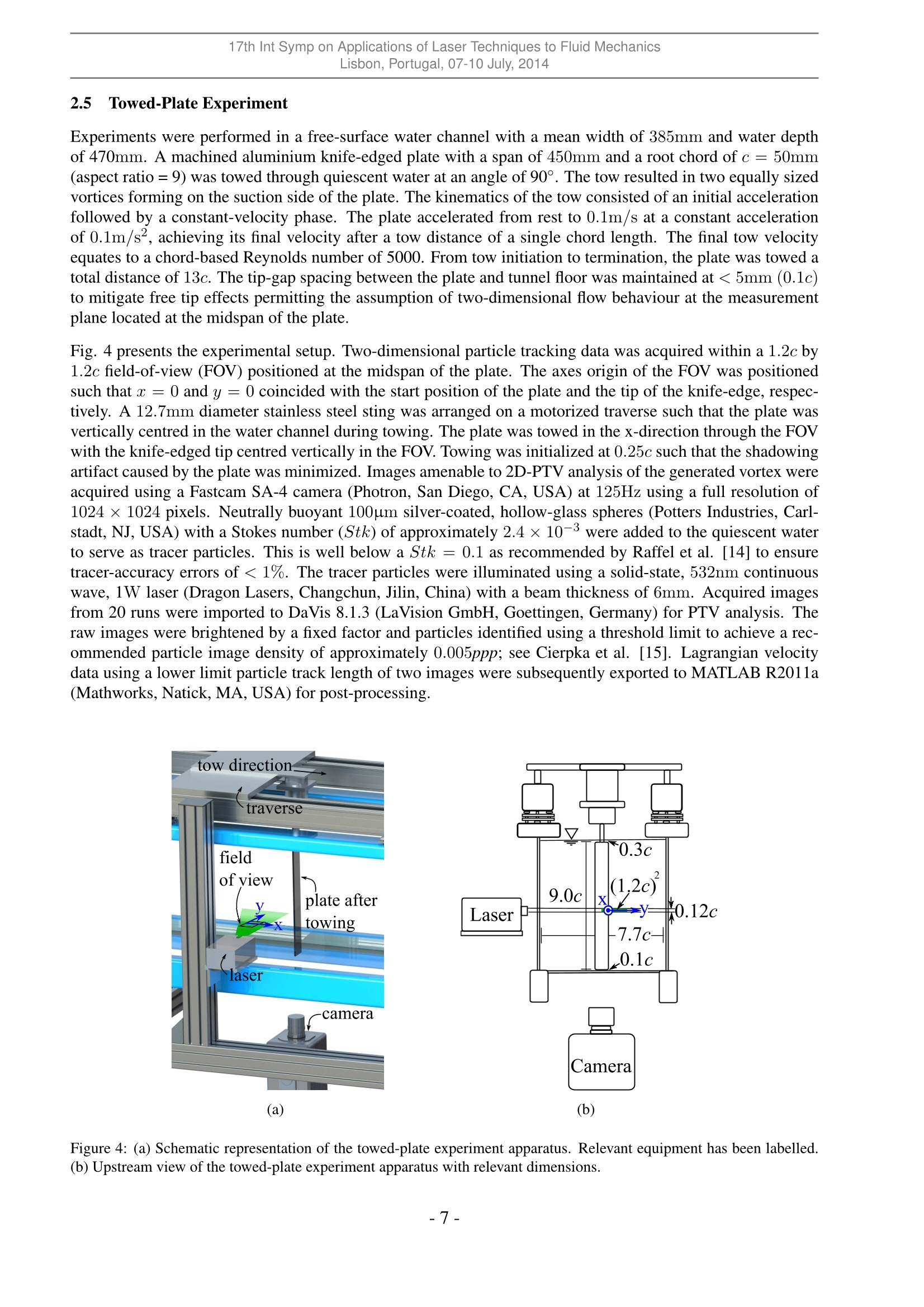
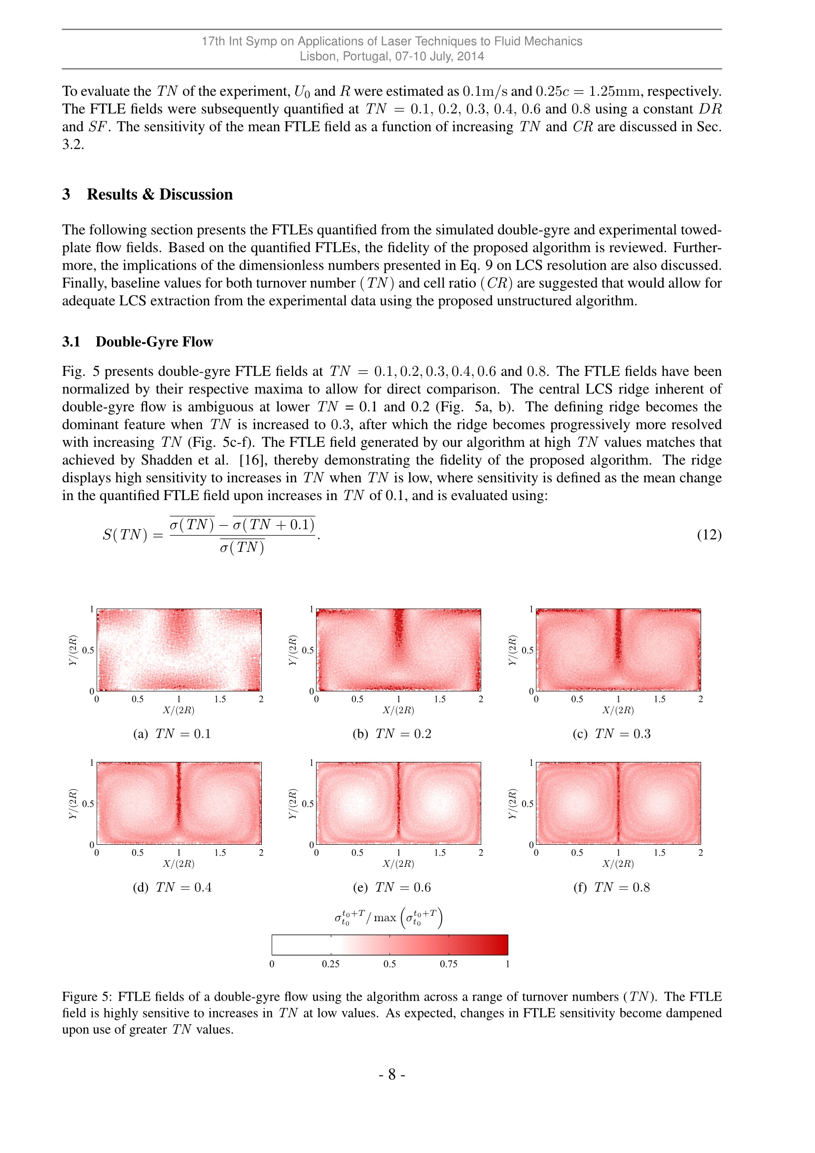
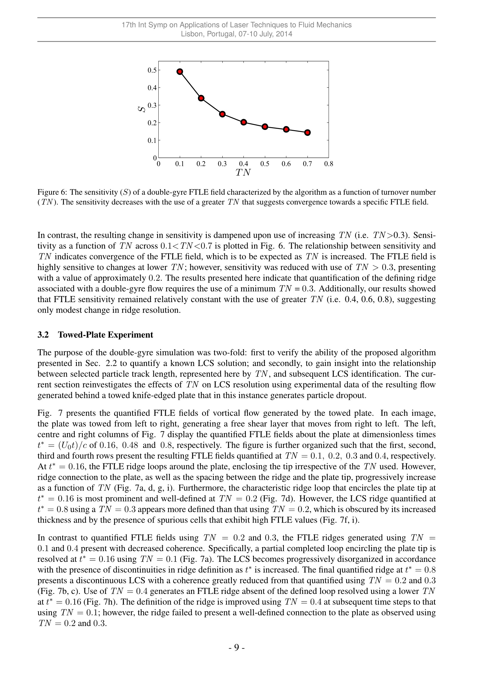
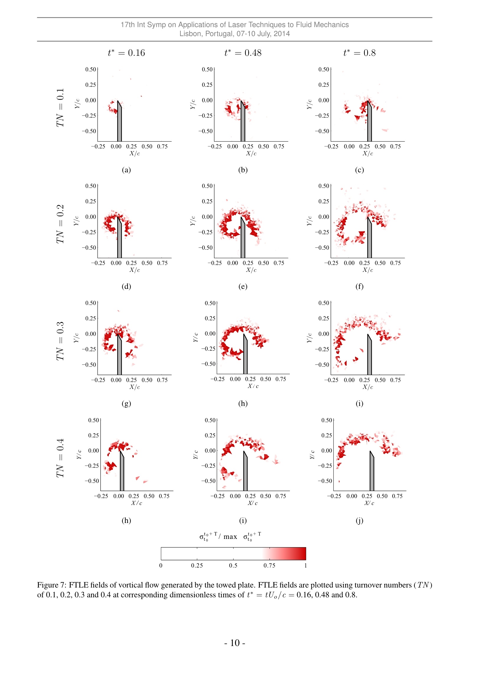
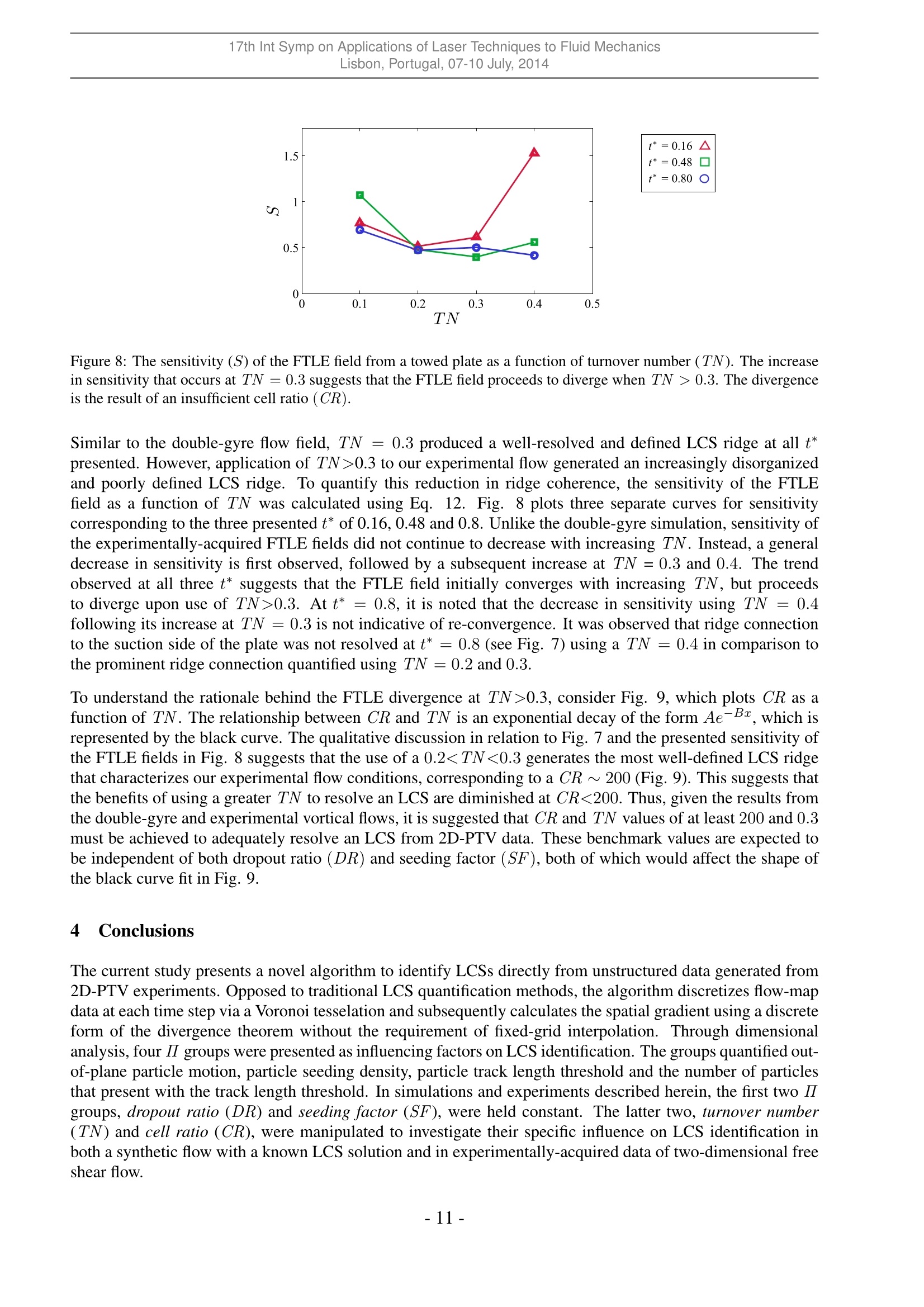
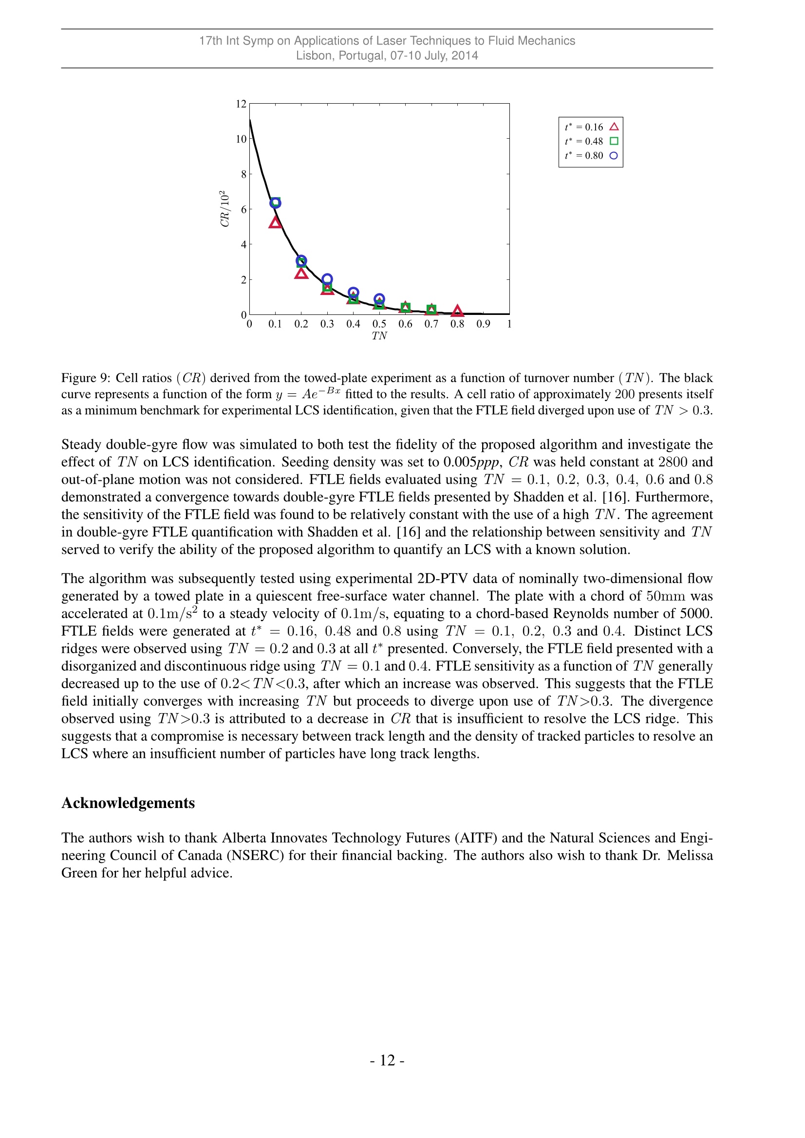
17th Int Symp on Applications of Laser Techniques to Fluid MechanicsLisbon， Portugal， 07-10 July， 2014 The Identification of Lagrangian Coherent Structures in a NominallyTwo-Dimensoinal Shear Flow via Lagrangian Particle Tracking Giuseppe A. Rosil， Andrew M. Walker and David E. Rival 1： Department of Mechanical Engineering， University of Calgary， Calgary， Canada*corresponding author： garosi@ucalgary.ca Abstract： The quantification of Lagrangian Coherent Structures (LCS) has been investigated using a novel algorithmbased on the tesselation of unstructured data points. The applicability of such an algorithm in resolving an LCS wasfirst tested using a synthetically-generated double-gyre flow with a known LCS solution. Subsequently， the algorithmwas tested on experimental data acquired using two-dimensional particle tracking velocimetry (2D-PTV) of a nominallytwo-dimensional free shear flow. To quantify factors linked to accurate LCS identification， dimensionless parameters aredeveloped to characterize their relationship to LCS resolution. Specifically， the study considers turnover number (TN)，which is defined here as the fraction of the particle track length to the vortical time scale， and cell ratio (CR)， whichcan be thought of as the relative density of particles with long track lengths per characteristic vortex length scale. Whenexamining the double-gyre finite-time Lyapunov exponent (FTLE) field， as expected， the resolution of the well-definedridge improved with increasing TN. Upon use of tracks lengths >30% of the overall vortex time scale， only modest im-provement in ridge resolution was observed. The LCS of the experimental data set was well-resolved using track lengthson the order of 20-30% of the vortex time scale. However， the use of greater TN values presented LCSs with an increas-ingly disordered coherence suggesting an inadequate particle count to accurately define the structure. Additionally， anexponential relationship was observed between CR and TN. This suggests that a compromise must be made betweentrack length and the density of tracked particles to adequately resolve an LCS where an insufficient number of particleshave long track lengths. 1 Introduction The ability to identify independent regions of coherent motion， or coherent structures， within temporally andspatially resolved flow data is essential in the study of unsteady flows. Technological limitations of earlyoptical measurements have resulted in the acquisition of flow fields using an Eulerian framework. As a con-sequence， traditional methods of coherent-structure identification relies on the input of Eulerian data. Theoriginal Eulerian-based technique was the Q-criterion developed by Hunt et al. [1]. More recent techniquesinclude the A-criterion developed by Chong et al. [2]， and the swirling-strength and I criteria， both developedspecifically for vortices by Zhou et al. [3] and Graftieaux et al. [4]，respectively. The commonality betweenall Eulerian identification methods is their reliance on the decomposition of the velocity-gradient tensor Vuinto the summation of the rate-of-strain and vorticity tensors， 2 and S， respectively. The eigenvalues of Sand ， and consequentially the coherent structures that the above techniques would identify， are invariant withGalilean-frame changes. Although Eulerian-based coherent-structure identification is widely used， Eulerian coherent structures (ELSs)suffer from three deficiencies. Firstly， ELSs are reference-frame dependent whereupon a change would beobserved for a transformation that involves acceleration； see Haller [5]. ELSs are also subject to user-definedthresholds leading to high subjectivity in structure boundary identification； see Green et al. [6]. Finally， thegeneration and breakdown of ELSs is purely speculative since one lacks the flow history of the fluid that com-prises the structure. In contrast， coherent structures identified from Lagrangian data， known as Lagrangiancoherent structures (LCSs)， do not suffer from the aforementioned deficiencies. LCSs are identified as regionsof extrema or inflection within a frame-invariant quantification of flow-map strain， which results in the iden-tification of structures unaffected by frame transformations， eliminating the need of a user-defined threshold.Additionally， Lagrangian data provides the flow history of particles， which in turn yields further insight into the generation and breakdown of coherent structures. Current state-of-the-art methods of LCS identificationinvolve using the smallest eigenvalue of the Cauchy-Green strain tensor (Peacock and Haller [7]) or the iden-tification of“black-holevortices， which are regions contained by manifolds of invariant tangential strain； seeHaller [8]. Regardless of the selected LCS identification method， the data at one’s disposal must be comprised of tracksof equal length that start and end concurrently， providing temporally homogeneous data. Acquiring such datafrom experiments is currently unfeasible， thus making the identification of LCSs from experimentally acquiredLagrangian data challenging. The inherent inhomogeneity of experimental Lagrangian data sets results ina coarse strain field， which in turn can obscure the LCSs contained therein. In the particular case of two-dimensional particle tracking velocimetry (2D-PTV)， the method is further limited by out-of-plane particlemotion that causes pathline breakage； see Raben et al. [9] and Brunton and Rowley [10]. Three-dimensionalmeasurement techniques can potentially reduce pathline-breakage effects， given that the out-of-plane particlemotion can be accurately quantified. However， there are numerous environments where the acquisition of three-dimensional Lagrangian measurements are highly challenging or unfeasible. Thus， it would be advantageousto discern when the three-dimensionality of nominally two-dimensional flows are negligible such that two-dimensional Lagrangian measurements are capable of accurately capturing LCS structures. Traditional methods of LCS identification from finite-time Lyapunov exponents (FTLE) are associated withhigh computational cost. Raben et al. [9] demonstrated that particle-tracking flow-map compilation (FMC)，which utilizes recorded particle images to represent Lagrangian flow tracers， generates more accurate estimatesof the FTLE flow field， specifically when seeding density is low. Opposed to past approaches that utilizevelocity-field integration， FMC is computationally more accurate through elimination of numerical integration.However， to compute FTLEs， the FMC approach requires interpolation of irregularly sampled spatial data ontoa rectilinear grid. With that in mind， the main thrust of the present study is the development of an FTLEcomputation method that uses unstructured Lagrangian data and excludes the use of interpolation to quantifyan LCS using two-dimensional measurement techniques in a nominally two-dimensional flow. The objectivesof the present study are two-fold. First， we wish to test the performance of our novel LCS identificationalgorithm that incorporates the use of unstructured Lagrangian data. Opposed to traditional approaches thatrely on fixed，structured grid interpolation， we present a new algorithm that utilizes Lagrangian velocity datain its unstructured spatial form to quantify an LCS through FTLE computation. To verify this approach，our developed algorithm is first tested using a synthetically-generated flow field with a known LCS solution.Subsequently， our algorithm is applied to experimental data acquired from flow generated by a towed knife-edged plate through quiescent fluid in a free-surface water channel. The accurate resolution of an LCS from experimental data is predicated on particle track length and the numberof particles that present with such lengths. Ideally， an infinite number of particles would be tracked witha length equal to the full time domain of the measurement. However， in any experiment， the number ofparticles that are tracked across a specific threshold time is both finite and decays exponentially as the tracklength threshold is increased. This exponential decay， from here forward referred to as particle dropout， waspresented by Schanz et al. [11] in reference to their "Shake-The-Box”evaluation approach to particle-basedtomographic data using a three-dimensional measurement approach. It is intuitive then that this exponentialparticle-dropout decay would be more acute using two-dimensional measurement approaches such as that usedhere. Furthermore， the approach of Schanz et al. [11] permits the tracking of individual particles at pixeldensities associated with tomographic PIV， increasing the number of available particles that present with longtrack lengths over traditional PTV approaches. Although an attractive measurement approach， imaging atsuch densities is not feasible in certain environments. We fully expect that our experimental data will presentwith few particle tracks that span the full time domain of our measurement. It is our second objective thento quantify the ability to characterize an LCS using Lagrangian experimental data upon the modification ofparticle track length and correspondingly， particle count. This will be achieved using a sensitivity analysisthrough the modification of track length to identify the minimum， non-dimensional track length required toquantify the LCS of our nominally two-dimensional experimental flow. The following describes our developed method of LCS quantification using a spatially unstructured grid andthe subsequent application of this algorithm to both synthetically-generated and experimental data sets. First， a detailed overview of the method is described followed by a description of both the synthetic data set witha known LCS solution and the experimental methods used to acquire 2D-PTV amenable images. Detailedanalysis and demonstration of this approach to double-gyre and experimental vortical flows is presented alongwith a sensitivity analysis of LCS identification as a function of dimensionless track length. 2Methods The current section explains the workings of our LCS algorithm using unstructured spatial data， followed by adescription of our simulated and experimental test cases. 2.1 FTLE Computation The FTLE measures the maximum linearized growth rate of distance between initially adjacent particlestracked over a finite time period. This requires the calculation of the Cauchy-Green (Cij) deformation ten-sor， which is defined as： where Voto+ is the gradient of the flow map to that maps fluid elements tracked at time to to theirfinal position at time to + T via Lagrangian particle tracking. Note that (V)* denotes the transpose ofvoto+. In two-dimensional flow， Vto+can be represented as： where the vectors [Xt， Yto] and [Xto+T Yto+T] represent the original and final positions of the particles. Subse-quently， identification of the highest eigenvalue (Xmaa) from the deformation tensor corresponds to maximumstretching whereupon the FTLE field (a) is given by： Computed FTLE maxima identified as distinct ridges are used to quantify the LCSs， which represent barriersto fluid flow that partition regions with unique dynamical behaviour (Espa et al. [12]). 2.2 LCS Determination from Unstructured Spatial Data The successful identification of LCSs depends on the accuracy in calculating the spatial gradient of Voto+，see Eq. 2. Thus， the ability to calculate spatial gradients is a necessary precursor to the successful identificationof LCSs using unstructured data. The following describes the development of such an algorithm to calculatethe necessary spatial derivatives. A schematic representative of a PTV time step is presented in Fig. 1(a). At the current time step (to)， Nparticles located at positions [Xto Yto] are tracked and an associated arbitrary scalar (A) is measured. From thedata， the spatial gradient of A (V(A)) is calculated. Voronoi tesselation is performed towards this end， whichresults in a collection of polygoncells that each enclose a single particle located at the centroid of the cell； seeFig. 1(a). Fig. 1(a) focuses on a single particle (P) and its respective cell (II) outlined in red. II in this instancerepresents a bounded cell that is surrounded by particles in such a manner that all cell faces have finite lengths.Along the periphery of any flow field， there will unavoidably exist particles that are insufficiently surroundedby other particles， referred to as unbounded cells where one or more faces have infinite lengths. Bounded andunbounded cells are represented by filled and unfilled circles respectively in Fig. 1. (a) Figure 1： (a) A representative time step of PTV data discretized via Voronoi tesselation. A scalar field (A) has beenmeasured for particles located at [Xto Yto]. Particles are enclosed by Voronoi cells (II) with areas (2). Empty and filledcircles indicate unbounded and bounded particles， respectively. (b) Geometric features of cell II pertaining to particle P.II is neighboured by a set of particles enumerated by I， whose locations Ar， have been measured. The side lengths thatII shares with cells enclosing particles I are denoted as lr and the distances between P and particles I are denoted as dr.The triangle enclosed by lr and P is Ar =drlr. We focus specifically on the geometry of II and its relation to its neighbouring particles and cells. Fig. 1(b)shows both P， II and neighbouring particles of P. II presents with an area (2) and consists of J faces andJ neighbouring cells that each enclose an individual particle. The neighbouring particles of P， as well as thefaces that cell II share with its corresponding neighbouring cells are enumerated by I. Thus， the lengths of thefaces shared by cell II and cells I and the distance between particle P and particles I are donated by lr and dI，respectively. If P is surrounded by an infinite number of particles， II would form a smooth contour. Also， VA would berelated to A along contour II through the divergence theorem： where n is a unit vector pointing normal and outwards from II. It is assumed here that cell II is sufficientlysmall such that VA is constant throughout . This assumption simplifies Eq. 4 to： Since the data is discrete，the path integral is replaced by a sum along all J faces of II， i.e.： where nr is a unit vector pointing normal to face I and AF，I is A evaluated along face I. A similar result ispresented in Hyman et al.，[13]. It is assumed that all lr are sufficiently small such that A may be assumedconstant along each face. A at each face is therefore approximated as a linear interpolation between Ap at Pand Ar at particle I. Given the inherent geometry of the Voronoi cells， this linear approximation simplifies toAF，I =(Ap+Ar). Furthermore， can be divided into J triangles where the vertices of each triangle arelocated at P and at the end points of a single face I. This allows to be represented as 2=Zi=i(lrdr). Given the simplifications described above， Eq. 6 can be written in the following discretized form： Note that Eq. 7 is only valid for two-dimensional flow fields and that modifications are required for applicationto three-dimensional flows. To determine a component of V(A)， nr is replaced by a dot product between niand the component of interest. Thus， the sc and y components of V(A) are： To calculate the spatial derivatives necessary to generate Voto+， A may be replaced by Xto+T and Yto+Tsince A represents a generic scalar field. It must also be noted that Voto+ can only be calculated at boundedparticles. The use of Eq. 7 is invalid and undefined for unbounded particles given their association with lr，which in this case are equal to infinity. 2.3 Non-Dimensional Parameters for Track Length Threshold As described in the introduction， accurate LCS identification is dependent on two competing factors： the se-lected threshold track length and the number of particles that present with such a length. Two non-dimensionalparameters are presented herein that are used throughout the current study to quantify both factors. Consider a two-dimensional ubiquitous shear flow shown schematically in Fig. 2. A fluid flows over anobstruction (thick solid line) at a uniform velocity (Uo). A resulting shear layer forms that divides the flow intoan irrotational region and a recirculation region， hereafter referred to as the vortex. The vortex has a radius (R)and mean tangential velocity along its periphery (Us). Superimposed onto the bulk two-dimensional flow areout-of-plane motions with a velocity scale (U_). Two-dimensional Lagrangian particle tracking with a seedingdensity (d in m-2) is performed within a laser sheet of thickness (l) to quantify the flow field. Particles with atemporal track length (T) are used to calculate the FTLE field， which increases the inter-particle spacing fromapproximately √dto e，where e is the inter-particle spacing between tracked particles. It is assumed herethat Us ~ Uo and that the vortex is contained within a contour of length 2m R. Furthermore， it is assumed that (a) (b) Figure 2： (a) Cross-sectional and (b) upstream views of a shear-layer flow downstream of a two-dimensional obstruction.Fluid travelling at a uniform velocity (Uo) flows over an obstruction leading to the development of a recirculation regionof radius (R) with a mean tangential velocity(Us). Thick solid lines represent the obstruction， while thick dashed linesrepresent a solid surface or a line of symmetry. Two-dimensional Lagrangian particle-tracking data was acquired usinga seeding density (d) and a laser sheet of thickness (). Particles that are tracked with minimum length (T) and aninter-particle spacing (E) are selected for LCS characterization. Superimposed onto the bulk two-dimensional flow areout-of-plane motions with a velocity scale (U_). Velocities and distances are represented by single- and double-headedarrows， respectively. U is proportional to the root-mean-square of the out-of-plane fluctuations，which is denoted as Vw’w’. Fromdimensional analysis， the mean error of the FTLE field (E) is a function of four II groups： Each II group can be ascribed a physical meaning. Ii， or the dropout ratio (DR)， approximates the timerequired for a fluid parcel positioned at the centre of the laser sheet to move through the sheet that is subse-quently non-dimensionalized by T.nR’represents the area of the vortex， while d-1approximates the meanarea of particle-enclosing cells (Sec. 2.2) when threshold T is not applied to the data. Thus， Il2， referred tohere as the seeding factor (SF)， approximates the number of data nodes within the vortex when threshold Tis not applied. IIs and II4 are dimensionless representations of threshold T and the number of particles thatpresent with the specified track length， respectively. Specifically， IIs represents the number of times a particlelocated at the periphery circulates around the vortex and as such will be referred as the turnover number (TN).II4 approximates the area ratio between the mean particle cell and the vortex and will be referred to as the cellratio(CR). 2.4AAlgorithm Verification via Double-Gyre Flow To verify the algorithm presented in Sec 2.2， the FTLE field of a data set with a known solution was calculated.Specifically， a double-gyre flow field consisting of confined counter-rotating vortices that represents a canonicaltest solution for LCS identification was generated using MATLAB R2011a (Mathworks， Natick， MA， USA)(Fig. 3).Between D/2R=[0，2]×0，1] the flow is described by the stream-function： where R represents the horizontal span of each vortex. Here， the X andY components of the vector field (UandV，respectively) are defined as： The above described domain was discretized into 2.0×106 pixels and seeded with 10000 particles in randompositions equating to a d=0.005 particles-per-pixel (ppp) or equivalently， d=5000 particles/(2R)2. Particletrack length was incrementally increased and the corresponding FTLE field was evaluated. As discussed pre-viously， the number of tracks present at a certain threshold length will decrease as the threshold is increased.However， to evaluate the convergence of the code and understand the dependence of E with TN， particledropout was not permitted. This resulted in a SF of 3900 and a constant CR of 2800. Out-of-plane motionwas not considered (i.e. DR=0). The FTLE field was evaluated using TN =0.1，0.2， 0.3， 0.4，0.6 and 0.8.The resulting FTLE field and the sensitivity of the FTLE field as a function of increasing TN are presented inSec. 3.1. Figure 3： Velocity field of a steady-state double-gyre flow. 2.5 Towed-Plate Experiment Experiments were performed in a free-surface water channel with a mean width of 385mm and water depthof 470mm. A machined aluminium knife-edged plate with a span of 450mm and a root chord of c= 50mm(aspect ratio=9) was towed through quiescent water at an angle of 90°. The tow resulted in two equally sizedvortices forming on the suction side of the plate. The kinematics of the tow consisted of an initial accelerationfollowed by a constant-velocity phase. The plate accelerated from rest to 0.1m/s at a constant accelerationof 0.1m/s， achieving its final velocity after a tow distance of a single chord length. The final tow velocityequates to a chord-based Reynolds number of 5000. From tow initiation to termination， the plate was towed atotal distance of 13c. The tip-gap spacing between the plate and tunnel floor was maintained at <5mm (0.1c)to mitigate free tip effects permitting the assumption of two-dimensional flow behaviour at the measurementplane located at the midspan of the plate. Fig. 4 presents the experimental setup. Two-dimensional particle tracking data was acquired within a 1.2c by1.2c field-of-view (FOV) positioned at the midspan of the plate. The axes origin of the FOV was positionedsuch that x =0 and y = 0 coincided with the start position of the plate and the tip of the knife-edge， respec-tively. A 12.7mm diameter stainless steel sting was arranged on a motorized traverse such that the plate wasvertically centred in the water channel during towing. The plate was towed in the x-direction through the FOVwith the knife-edged tip centred vertically in the FOV. Towing was initialized at 0.25c such that the shadowingartifact caused by the plate was minimized. Images amenable to 2D-PTV analysis of the generated vortex wereacquired using a Fastcam SA-4 camera (Photron， San Diego， CA， USA) at 125Hz using a full resolution of1024×1024 pixels. Neutrally buoyant 100um silver-coated， hollow-glass spheres (Potters Industries， Carl-stadt， NJ， USA) with a Stokes number (Stk) of approximately 2.4×10-3 were added to the quiescent waterto serve as tracer particles. This is well below a Stk =0.1 as recommended by Raffel et al. [14] to ensuretracer-accuracy errors of < 1%. The tracer particles were illuminated using a solid-state， 532nm continuouswave， 1W laser (Dragon Lasers， Changchun， Jilin， China) with a beam thickness of 6mm. Acquired imagesfrom 20 runs were imported to DaVis 8.1.3 (LaVision GmbH， Goettingen， Germany) for PTV analysis. Theraw images were brightened by a fixed factor and particles identified using a threshold limit to achieve a rec-ommended particle image density of approximately 0.005ppp； see Cierpka et al. [15]. Lagrangian velocitydata using a lower limit particle track length of two images were subsequently exported to MATLAB R2011a(Mathworks， Natick， MA， USA) for post-processing. (b) To evaluate the TN of the experiment， Uo and R were estimated as 0.1m/s and 0.25c =1.25mm，respectively.The FTLE fields were subsequently quantified at TN = 0.1，0.2，0.3， 0.4，0.6 and 0.8 using a constant DRand SF. The sensitivity of the mean FTLE field as a function of increasing TN and CR are discussed in Sec.3.2. 3 Results & Discussion The following section presents the FTLEs quantified from the simulated double-gyre and experimental towed-plate flow fields. Based on the quantified FTLEs， the fidelity of the proposed algorithm is reviewed. Further-more， the implications of the dimensionless numbers presented in Eq. 9 on LCS resolution are also discussed.Finally， baseline values for both turnover number (TN) and cell ratio (CR) are suggested that would allow foradequate LCS extraction from the experimental data using the proposed unstructured algorithm. 3.1 Double-Gyre Flow Fig. 5 presents double-gyre FTLE fields at TN = 0.1，0.2，0.3，0.4，0.6 and 0.8. The FTLE fields have beennormalized by their respective maxima to allow for direct comparison. The central LCS ridge inherent ofdouble-gyre flow is ambiguous at lower TN= 0.1 and 0.2 (Fig. 5a， b). The defining ridge becomes thedominant feature when TN is increased to 0.3， after which the ridge becomes progressively more resolvedwith increasing TN (Fig. 5c-f). The FTLE field generated by our algorithm at high TN values matches thatachieved by Shadden et al. [16]， thereby demonstrating the fidelity of the proposed algorithm. The ridgedisplays high sensitivity to increases in TN when TN is low， where sensitivity is defined as the mean changein the quantified FTLE field upon increases in TN of 0.1， and is evaluated using： Figure 5： FTLE fields of a double-gyre flow using the algorithm across a range of turnover numbers (TN). The FTLEfield is highly sensitive to increases in TN at low values. As expected， changes in FTLE sensitivity become dampenedupon use of greater TN values. Figure 6： The sensitivity (S) of a double-gyre FTLE field characterized by the algorithm as a function of turnover number(TN). The sensitivity decreases with the use of a greater TN that suggests convergence towards a specific FTLE field. In contrast， the resulting change in sensitivity is dampened upon use of increasing TN (i.e. TN>0.3). Sensi-tivity as a function of TN across 0.1 0.3， presentingwith a value of approximately 0.2. The results presented here indicate that quantification of the defining ridgeassociated with a double-gyre flow requires the use of a minimum TN=0.3. Additionally， our results showedthat FTLE sensitivity remained relatively constant with the use of greater TN (i.e. 0.4， 0.6，0.8)， suggestingonly modest change in ridge resolution. 3.2 Towed-Plate Experiment The purpose of the double-gyre simulation was two-fold： first to verify the ability of the proposed algorithmpresented in Sec. 2.2 to quantify a known LCS solution； and secondly， to gain insight into the relationshipbetween selected particle track length， represented here by TN， and subsequent LCS identification. The cur-rent section reinvestigates the effects of TN on LCS resolution using experimental data of the resulting flowgenerated behind a towed knife-edged plate that in this instance generates particle dropout. Fig. 7 presents the quantified FTLE fields of vortical flow generated by the towed plate. In each image，the plate was towed from left to right， generating a free shear layer that moves from right to left. The left，centre and right columns of Fig. 7 display the quantified FTLE fields about the plate at dimensionless timest* = (Uot)/c of 0.16， 0.48 and 0.8， respectively. The figure is further organized such that the first， second，third and fourth rows present the resulting FTLE fields quantified at TN=0.1，0.2，0.3 and 0.4， respectively.At t* = 0.16， the FTLE ridge loops around the plate， enclosing the tip irrespective of the TN used. However，ridge connection to the plate， as well as the spacing between the ridge and the plate tip， progressively increaseas a function of TN (Fig. 7a， d， g， i). Furthermore， the characteristic ridge loop that encircles the plate tip att* = 0.16 is most prominent and well-defined at TN =0.2 (Fig. 7d). However， the LCS ridge quantified att*=0.8 using a TN =0.3 appears more defined than that using TN =0.2， which is obscured by its increasedthickness and by the presence of spurious cells that exhibit high FTLE values (Fig. 7f， i). In contrast to quantified FTLE fields using TN =0.2 and 0.3， the FTLE ridges generated using TN =0.1 and 0.4 present with decreased coherence. Specifically， a partial completed loop encircling the plate tip isresolved at t* = 0.16 using TN =0.1 (Fig. 7a). The LCS becomes progressively disorganized in accordancewith the presence of discontinuities in ridge definition as t* is increased. The final quantified ridge at t*=0.8presents a discontinuous LCS with a coherence greatly reduced from that quantified using TN=0.2 and 0.3(Fig. 7b， c). Use of TN =0.4 generates an FTLE ridge absent of the defined loop resolved using a lower TNat t*=0.16 (Fig. 7h). The definition of the ridge is improved using TN=0.4 at subsequent time steps to thatusing TN =0.1； however， the ridge failed to present a well-defined connection to the plate as observed usingTN=0.2 and 0.3. t*=0.16 t*=0.48 (a) (b) (c) (d) (e) (f) 0.50 0.25 0.00 -0.25 -0.50 -0.250.000(.250.500.75 X/c (g) (h) (i) 10.50 0.50 0.25 0.25 寸0.00 0.00Ⅱ 之 -0.25 -0.25 -0.50 -0.50 -0.250(.0000.250.500.75 -0.255 0(.000.250.50 0.75 X/c X/c (h) oto+T/ max t 0 0.25 0.5 0.75 Figure 7： FTLE fields of vortical flow generated by the towed plate. FTLE fields are plotted using turnover numbers (TN)of 0.1， 0.2， 0.3 and 0.4 at corresponding dimensionless times of t* = tU。/c=0.16，0.48 and 0.8. Figure 8： The sensitivity (S) of the FTLE field from a towed plate as a function of turnover number (TN). The increasein sensitivity that occurs at TN=0.3 suggests that the FTLE field proceeds to diverge when TN >0.3. The divergenceis the result of an insufficient cell ratio (CR). Similar to the double-gyre flow field， TN = 0.3 produced a well-resolved and defined LCS ridge at all t*presented. However， application of TN>0.3 to our experimental flow generated an increasingly disorganizedand poorly defined LCS ridge. To quantify this reduction in ridge coherence， the sensitivity of the FTLEfield as a function of TN was calculated using Eq. 12. Fig. 8 plots three separate curves for sensitivitycorresponding to the three presented t* of 0.16， 0.48 and 0.8. Unlike the double-gyre simulation， sensitivity ofthe experimentally-acquired FTLE fields did not continue to decrease with increasing TN. Instead， a generaldecrease in sensitivity is first observed， followed by a subsequent increase at TN= 0.3 and 0.4. The trendobserved at all three t* suggests that the FTLE field initially converges with increasing TN， but proceedsto diverge upon use of TN>0.3. At t* = 0.8， it is noted that the decrease in sensitivity using TN = 0.4following its increase at TN =0.3 is not indicative of re-convergence. It was observed that ridge connectionto the suction side of the plate was not resolved at t*=0.8 (see Fig. 7) using a TN = 0.4 in comparison tothe prominent ridge connection quantified using TN = 0.2 and 0.3. To understand the rationale behind the FTLE divergence at TN>0.3， consider Fig. 9， which plots CR as afunction of TN. The relationship between CR and TN is an exponential decay of the form Ae-Bx， which isrepresented by the black curve. The qualitative discussion in relation to Fig. 7 and the presented sensitivity ofthe FTLE fields in Fig. 8 suggests that the use of a 0.20.3. Steady double-gyre flow was simulated to both test the fidelity of the proposed algorithm and investigate theeffect of TN on LCS identification. Seeding density was set to 0.005ppp，CR was held constant at 2800 andout-of-plane motion was not considered. FTLE fields evaluated using TN =0.1， 0.2，0.3，0.4， 0.6 and 0.8demonstrated a convergence towards double-gyre FTLE fields presented by Shadden et al.[16]. Furthermore，the sensitivity of the FTLE field was found to be relatively constant with the use of a high TN. The agreementin double-gyre FTLE quantification with Shadden et al. [16] and the relationship between sensitivity and TNserved to verify the ability of the proposed algorithm to quantify an LCS with a known solution. The algorithm was subsequently tested using experimental 2D-PTV data of nominally two-dimensional flowgenerated by a towed plate in a quiescent free-surface water channel. The plate with a chord of 50mm wasaccelerated at 0.1m/s to a steady velocity of 0.1m/s， equating to a chord-based Reynolds number of 5000.FTLE fields were generated at t* = 0.16， 0.48 and 0.8 using TN = 0.1， 0.2， 0.3 and 0.4. Distinct LCSridges were observed using TN =0.2 and 0.3 at all t* presented. Conversely， the FTLE field presented with adisorganized and discontinuous ridge using TN = 0.1 and 0.4. FTLE sensitivity as a function of TN generallydecreased up to the use of 0.20.3. The divergenceobserved using TN>0.3 is attributed to a decrease in CR that is insufficient to resolve the LCS ridge. Thissuggests that a compromise is necessary between track length and the density of tracked particles to resolve anLCS where an insufficient number of particles have long track lengths. Acknowledgements The authors wish to thank Alberta Innovates Technology Futures (AITF) and the Natural Sciences and Engi-neering Council of Canada (NSERC) for their financial backing. The authors also wish to thank Dr. MelissaGreen for her helpful advice. ( References ) ( [1] J. C. R. Hunt， A. A. Wray， and M. Moin. Ed d ies， str e ams and convergence zones in turbulent flow s .Center for Turbulence Research， 1988. ) ( [2] M . S. Chong， A. E. P e rry， a n d B. J. Cantwell. A general classification of a three-dimensional flow fields.Physics of Fluids， 2：765- 7 77，1990. ) ( [3] J. Zhou， R. J. Adrian， S. Balachandar， and T . M. Kendall. Mechanisms for generating coherent pac k etsof hairpin vortices in channel flow. Journal of Fluid Mechanics， 3 8 7：353-396， 199 9 . ) ( [4] L. Graftieaux， M . Michard， a n d N. Grosjean. Combining piv， pod and vortex identification algorithmsfor the study of unsteady turbulent swirling flow s . Measurement Science and Technology， 12：1422-1429， 2001. ) ( [5] G. H aller. An objective definition of a vorte x .Journal of Fluid Mechanics， 525：1-26， 2005. ) ( [6] M. A. Green， C. W. Rowley， and G. H aller. Detection of l a grangian cohe r ent stru c tures in three-dimensionl turbulence. Journal of Fluid Mechanics， 572：111-120， 2007. ) ( [7] T. Peacock and G . Haller. Lagrangian coh e rent structures： The hidden skeleton of fl u id flows. Physi c sToday， 66(2)：41-47，2013. ) ( [8] G. Haller and F .J. B eron-Vera. C o herent lagrangian vortices： the black holes of turbulence. Journal ofFluid Mechanics， 731：1-10，2013. ) ( [9] S. G. Raben， S. D . Ross， and P . P. V lachos. C o mputation of finite time lyapunov exponents from timeresolved particle image velocimetry data. E xperiments in Fluids， 2013. ) ( [10] S. L. Brunton and C. W. R o wley. Fa s t computation of ftle fields for u n steady flows： A comparison ofmethods. Journal of Chaos， 20：1-12，2010. ) ( [11] D. Schanz， A. Schroder， S. Gesemann， D. Mich a elis， and B. Wieneke. “shake the box”： A highly efficientand accurate tomographic particle tracking velocimetry ( tomo-ptv) method using prediction of particlepositions. Proceedings of the 1 0th International Symposium on Particle Image Velocimetry. ) ( [12] A . E spa， M. G. B a das， S. Fortini， G. Querzoli， and A. Cenedese. A l agrangian investigation of the flowinside the left ventricle. European Journal of Mechanics B/Fluids， 35：9-19， 2012. ) ( [1 3 ] J. M. H yman， R. J. Knapp， and J. C. Scovel. Hi g h order finite volume approximations of differnetial operators on nonuniform grids. Physica D， 60：112-138， 1992. ) ( [14] M.Raffel， C. E . Willert， S . T. Wereley， and J. Kompenhans. Pa r ticle Image Velocimetry： A PracticalGuide. Springer， 2nd edition，2007. ) ( [15] C. Cierpka， B. L i itke， a nd C. J. K ahler. H igher order multi-frame particle tracking velocimetry. Experi-ments in Fluids， 54：1533， 2 013. ) ( [16] S . C. Shadden， F. Lekien， and J. E. Marsden. Definition and properties of lagrangian c oherent structuresfrom finite-time lyapunov exponents in two-dimensional aperiodic flows. Physica D， 212：271-304，2005. ) -- -- The quantification of Lagrangian Coherent Structures (LCS) has been investigated using a novel algorithm based on the tesselation of unstructured data points. The applicability of such an algorithm in resolving an LCS was first tested using a synthetically-generated double-gyre flow with a known LCS solution. Subsequently, the algorithm was tested on experimental data acquired using two-dimensional particle tracking velocimetry (2D-PTV) of a nominallytwo-dimensional free shear flow. To quantify factors linked to accurate LCS identification, dimensionless parameters are developed to characterize their relationship to LCS resolution. Specifically, the study considers turnover number (TN), which is defined here as the fraction of the particle track length to the vortical time scale, and cell ratio (CR), which can be thought of as the relative density of particles with long track lengths per characteristic vortex length scale. When examining the double-gyre finite-time Lyapunov exponent (FTLE) field, as expected, the resolution of the well-defined ridge improved with increasing TN. Upon use of tracks lengths >30% of the overall vortex time scale, only modest improvement in ridge resolution was observed. The LCS of the experimental data set was well-resolved using track lengths on the order of 20-30% of the vortex time scale. However, the use of greater TN values presented LCSs with an increasingly disordered coherence suggesting an inadequate particle count to accurately define the structure. Additionally, an exponential relationship was observed between CR and TN. This suggests that a compromise must be made betweentrack length and the density of tracked particles to adequately resolve an LCS where an insufficient number of particles have long track lengths.