流场中层析PTV和层析PIV检测方案(工作站及软件)

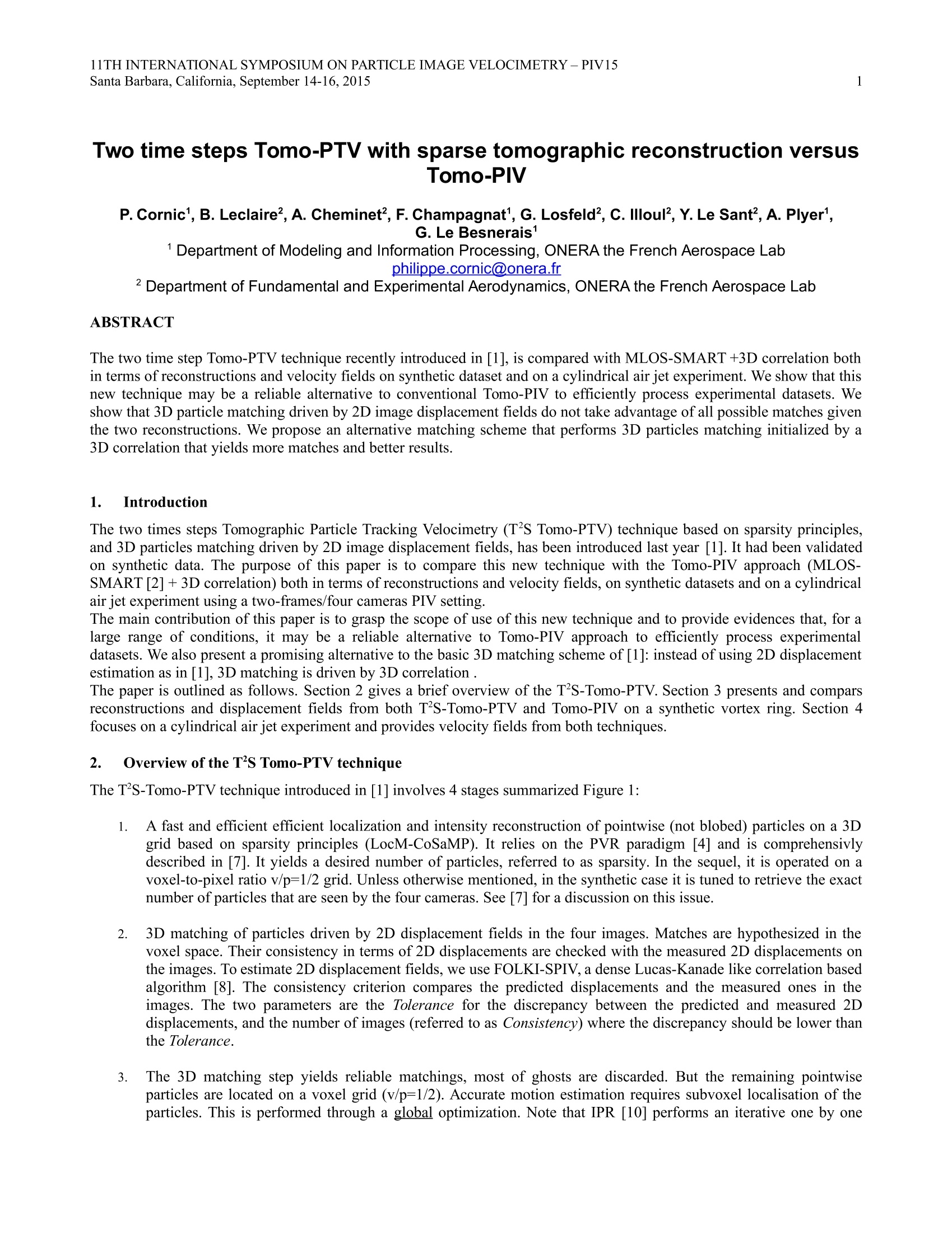
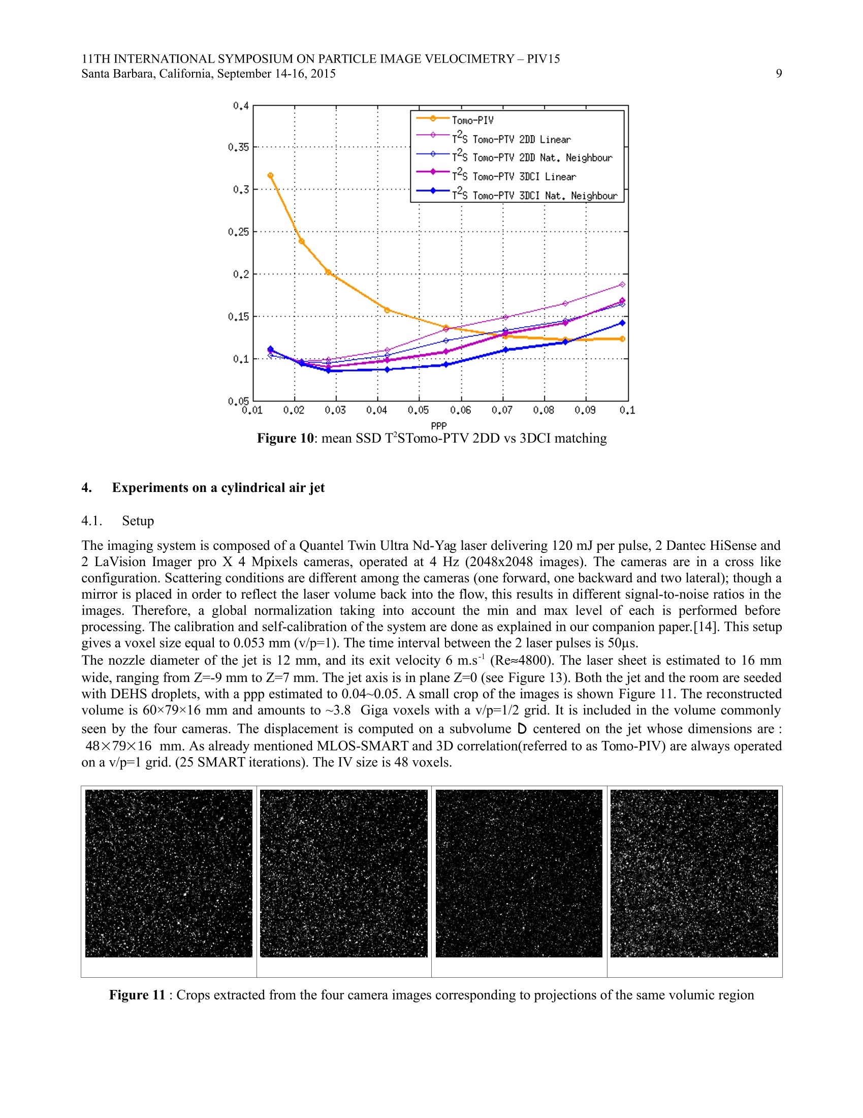
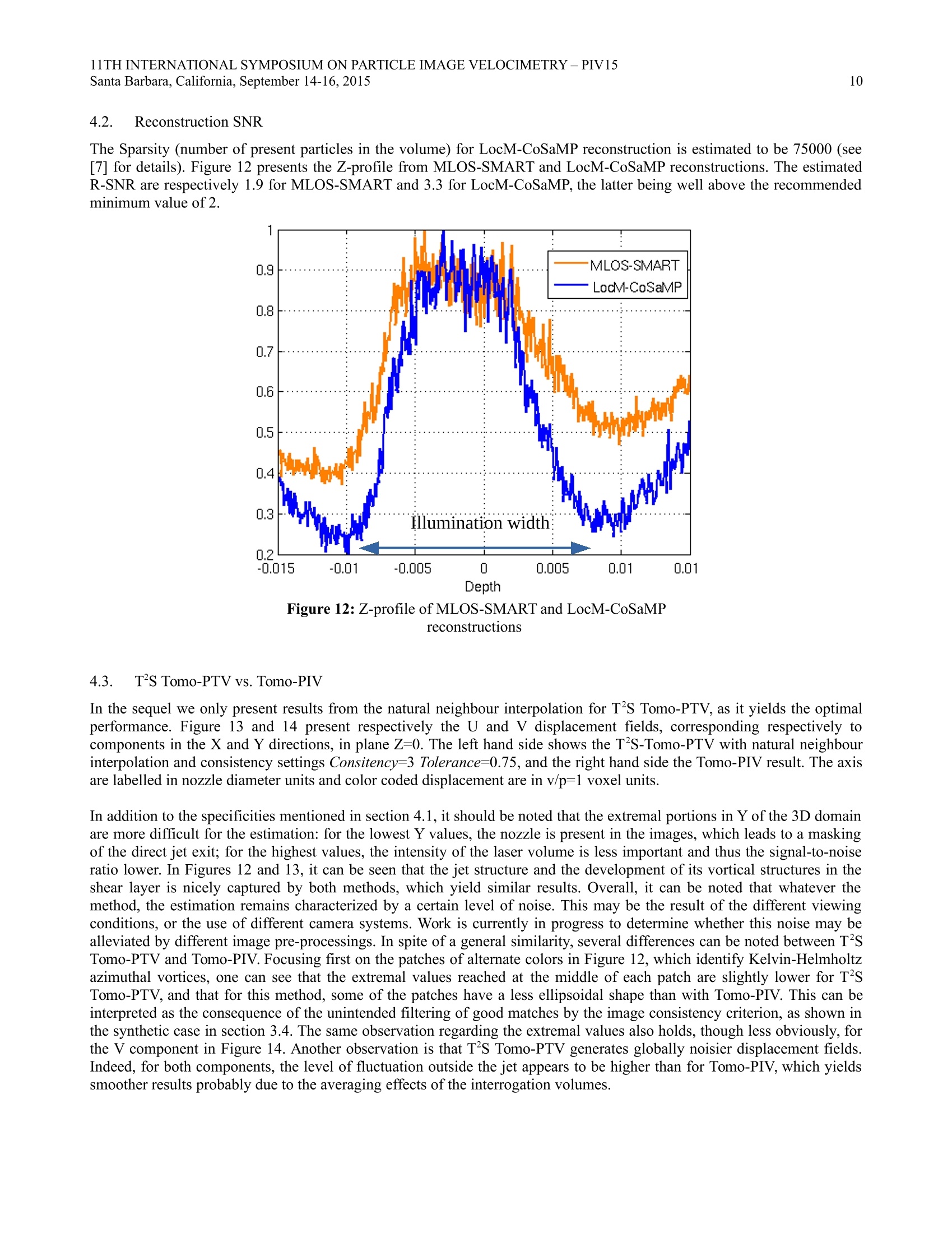
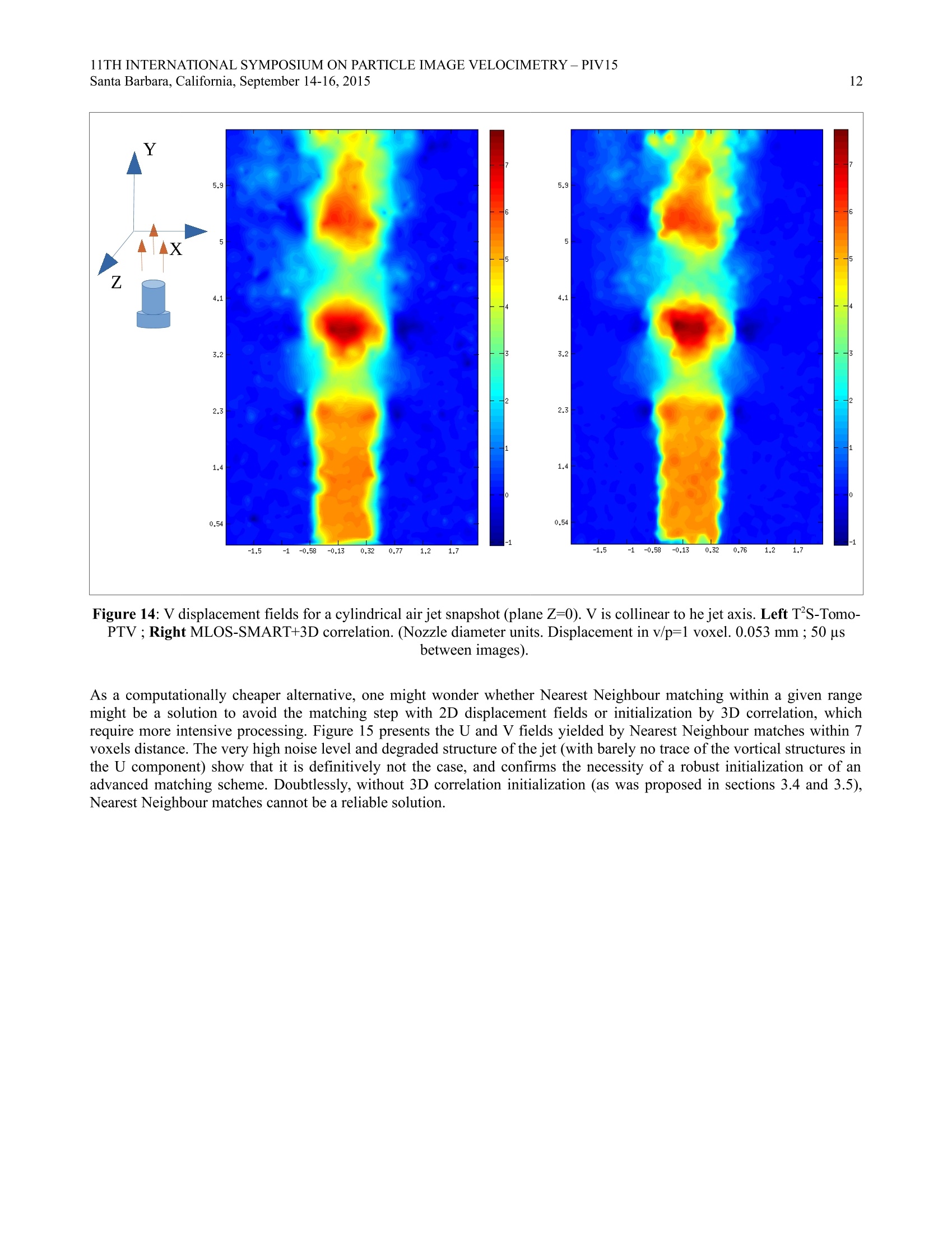
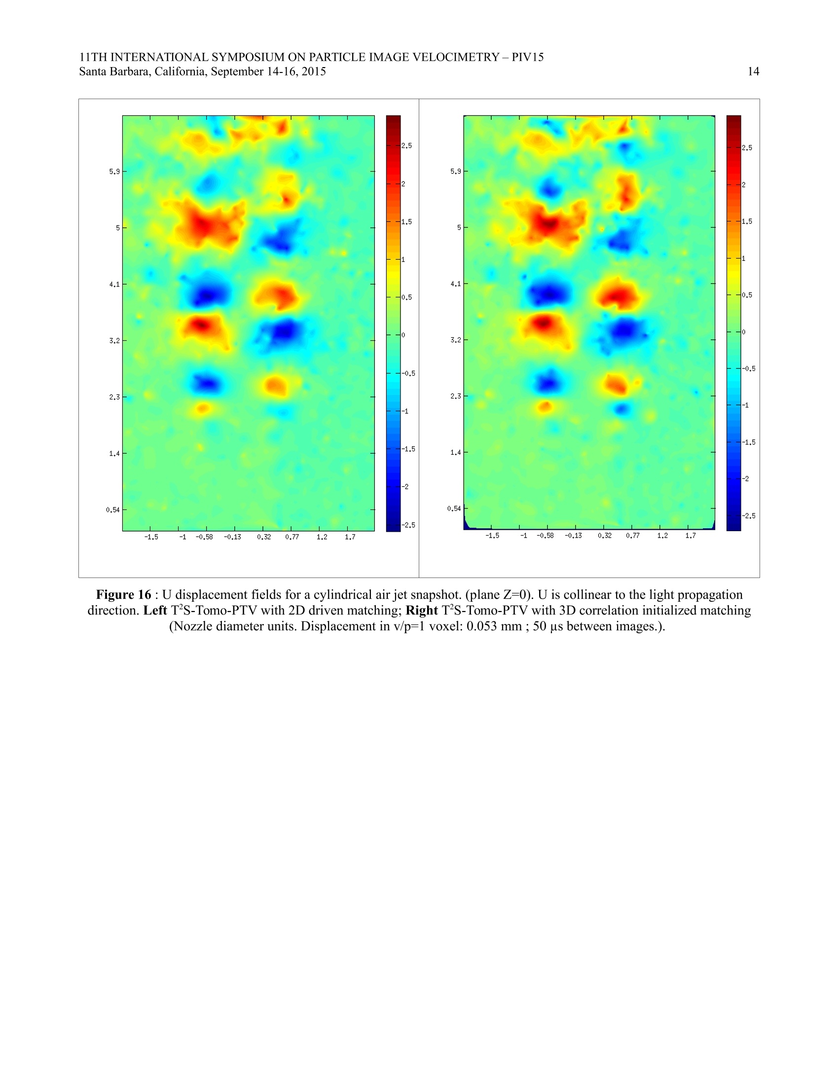
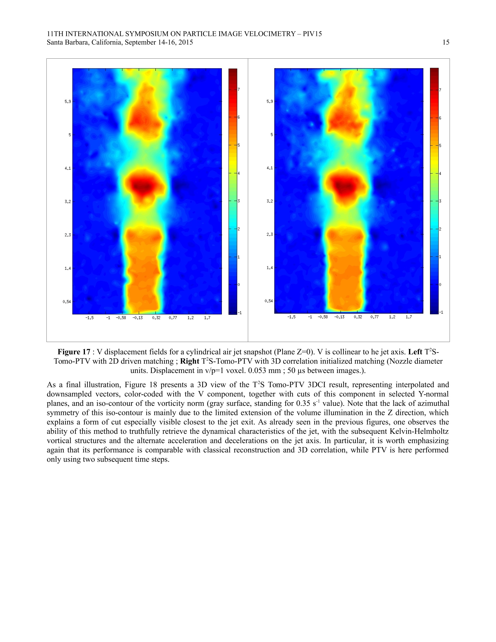
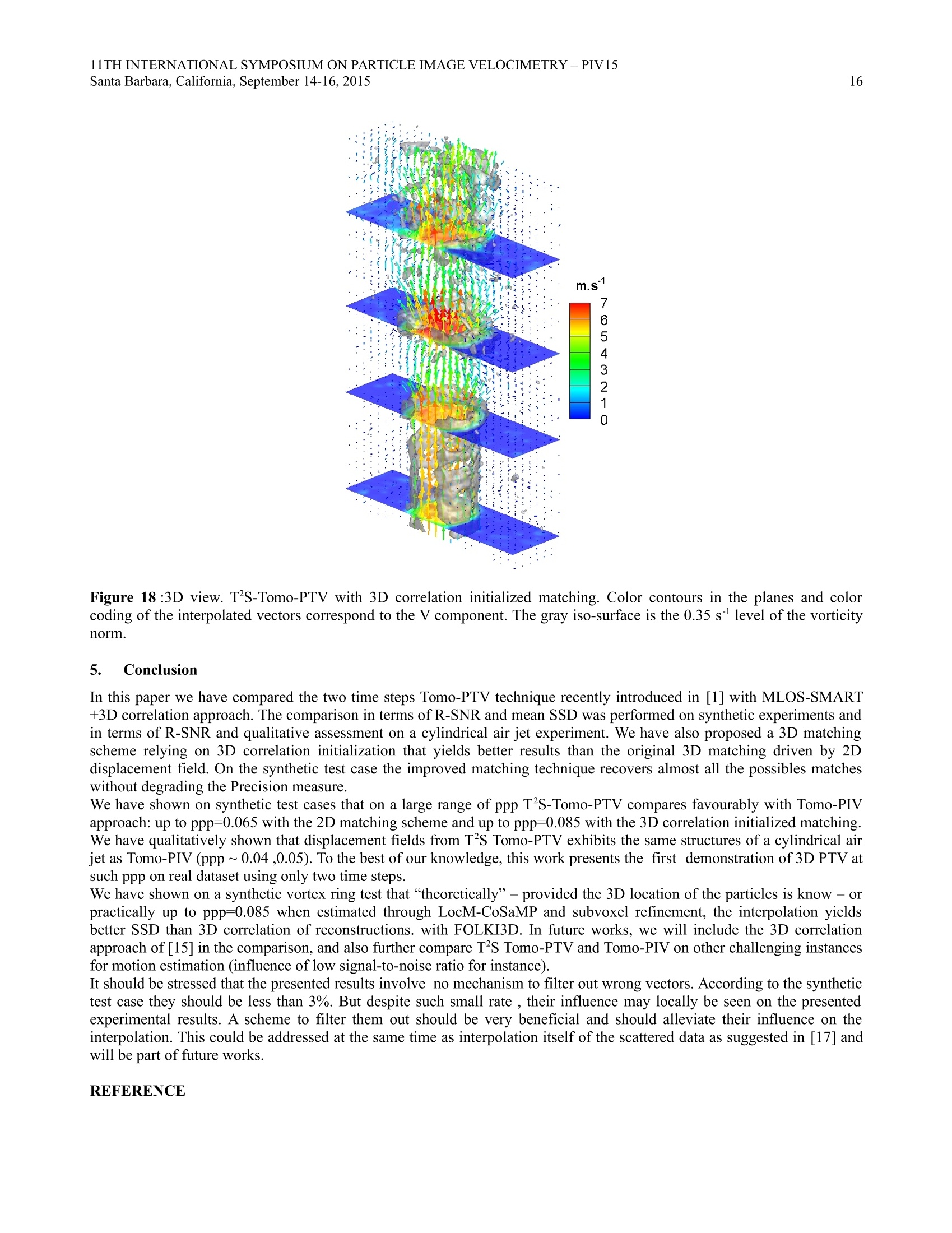
ResearchGateSee discussions， stats， and author profiles for this publication at： https：//www.researchgate.net/publication/282002670 11TH INTERNATIONAL SYMPOSIUM ON PARTICLE IMAGE VELOCIMETRY-PIV15Santa Barbara， California， September 14-16， 2015 Two time steps Tomo-PTV with sparse tomographic reconstruction versusTomo-PIV Conference Paper·September 2015 CITATIONS2 READS158 9 authors，including： Philippe Cornic The French Aerospace Lab ONERA 26 PUBLICATIONS 174 CITATIONS SEE PROFILE Adam Cheminet Sorbonne Universite 15 PUBLICATIONS 68 CITATIONS SEE PROFILE SEE PROFILE Some of the authors of this publication are also working on these related projects： Project 3D Background Oriented Schlieren View project Two time steps Tomo-PTV with sparse tomographic reconstruction versusTomo-PIV P. Cornic， B. Leclaire?， A. Cheminet?， F. Champagnat， G.Losfeld?， C. Illoul?， Y. Le Sant， A. Plyer，G.Le Besnerais1 Department of Fundamental and Experimental Aerodynamics，ONERA the French Aerospace Lab ABSTRACT The two time step Tomo-PTV technique recently introduced in [1]， is compared with MLOS-SMART +3D correlation bothin terms of reconstructions and velocity fields on synthetic dataset and on a cylindrical air jet experiment. We show that thisnew technique may be a reliable alternative to conventional Tomo-PIV to efficiently process experimental datasets. Weshow that 3D particle matching driven by 2D image displacement fields do not take advantage of all possible matches giventhe two reconstructions. We propose an alternative matching scheme that performs 3D particles matching initialized by a3D correlation that yields more matches and better results. Le Introduction The two times steps Tomographic Particle Tracking Velocimetry (T’S Tomo-PTV) technique based on sparsity principles，and 3D particles matching driven by 2D image displacement fields， has been introduced last year [1]. It had been validatedon synthetic data. The purpose of this paper is to compare this new technique with the Tomo-PIV approach (MLOS-SMART [2] +3D correlation) both in terms of reconstructions and velocity fields， on synthetic datasets and on a cylindricalair jet experiment using a two-frames/four cameras PIV setting. The main contribution of this paper is to grasp the scope ofuse of this new technique and to provide evidences that， for alarge range of conditions， it may be a reliable alternative to Tomo-PIV approach to efficiently process experimentaldatasets. We also present a promising alternative to the basic 3D matching scheme of [1]： instead of using 2D displacementestimation as in [1]， 3D matching is driven by 3D correlation. The paper is outlined as follows. Section2 gives a brief overview of the T?S-Tomo-PTV. Section 3 presents and comparsreconstructions and displacement fields from both T'S-Tomo-PTV and Tomo-PIV on a synthetic vortex ring. Section 4focuses on a cylindrical air jet experiment and provides velocity fields from both techniques. 2. Overview of the T’S Tomo-PTVtechnique The TS-Tomo-PTV technique introduced in [1] involves 4 stages summarized Figure 1： 1. A fast and efficient efficient localization and intensity reconstruction of pointwise (not blobed) particles on a 3Dgrid based on sparsity principles (LocM-CoSaMP). It relies on the PVR paradigm [4] and is comprehensivlydescribed in [7]. It yields a desired number of particles， referred to as sparsity. In the sequel， it is operated on avoxel-to-pixel ratio v/p=1/2 grid. Unless otherwise mentioned， in the synthetic case it is tuned to retrieve the exactnumber of particles that are seen by the four cameras. See [7] for a discussion on this issue. 2. 3D matching of particles driven by 2D displacement fields in the four images. Matches are hypothesized in thevoxel space. Their consistency in terms of 2D displacements are checked with the measured 2D displacements onthe images. To estimate 2D displacement fields， we use FOLKI-SPIV， a dense Lucas-Kanade like correlation basedalgorithm [8]. The consistency criterion compares the predicted displacements and the measured ones in theimages. The two parameters are the Tolerance for the discrepancy between the predicted and measured 2Ddisplacements， and the number of images (referred to as Consistency) where the discrepancy should be lower thanthe Tolerance. 3. The 3D matching step yields reliable matchings， most of ghosts are discarded. But the remaining pointwiseparticles are located on a voxel grid (v/p=1/2). Accurate motion estimation requires subvoxel localisation of theparticles. This is performed through a global optimization. Note that IPR [10] performs an iterative one by one optimization. The objective function to minimize is the sum of squared differences between predicted andrecorded images. Let E， and X， be the intensities and IR’ locations of the particles. x=(x，y) denotes any location in the imageplane， h is the compactly supported PSF function. F(x，) is the geometrical image of particle p in image j. Yj arethe recorded images. We look for： When the particles number exceeds a fixed number (a few tens of thousands) we turn to graph partitioning [11] toperform optimization on independent smaller subsets. 4. The displacements which are computed at the location of the particles at the first instant are interpolated on aregular grid through scattered data interpolation technique， to yield the final 3D displacement field. Step 3 ： Subvoxel refinement of matched particles Step 4 ： Interpolation on a 3D regular grid Figure 1： The four stages of the T’S Tomo-PTV technique. 3. Synthetic experiments 3.1. Setup A thorough description of our synthetic setup can be found in [3]，[4]. All our simulations involve four cameras， which arepositioned on a single side of the laser sheet at the vertices11)ofa2'2'2of a square of 1 meter side. They are positioned at 1 meter from the centre of the reconstructed volume located at (0，0，0) and point at it. The voxel-to-pixel ratio v/p=1leads to voxels of 0.1 mm side. The tracers particles are uniformly distributed in the 2cm width light sheet volume. As inreal datasets， a fraction of illuminated particles cannot be seen by all the cameras. The 1024x1024 images Y (j=1..4) are synthesised according to：Y(x)=E，h(x-F(X，))Pwhere x=(x，y) denotes any location in the image plane， h is the compactly supported PSF function， E， and X， are theintensity and 3D coordinates of particle p. E， is distributed according a gaussian law. F，(x，) is the geometrical image ofparticle p. A gaussian noise with zero mean and standard deviation 2 is added to the images (with negative values thresholded to zero).Its amplitude is thus about 5% relative to the maximum particle intensity. The displacement field considered is a vortex ring， similar to that considered by [5]， whose main section lies in the Z=Oplane. The radius of the ring is equal to 393 voxels and the maximum displacement is roughly equal to 3 voxels (in v/p =1unit). 3.2. Reconstruction： LocM-CoSaMP vs. MLOS-SMART The reconstruction of the 3D distribution and intensity of the illuminated particles is the critical step of 3D PIV. [7]compares LocM-CoSaMP and MLOS-SMART reconstructions in terms of quality factor， Precision and Recall. We focushere on the R-SNR defined as the ratio between the plateau and edge values of the reconstruction Z-profile [6]. Inexperiments a recommended minimum value is 2. MLOS-SMART is always operated on a v/p=1 grid with 25 SMARTiterations. The illuminated volume is 2 cm thick， from Z=-1cm to Z=1cm. For this synthetic experiment， the reconstructed volume isthe volume seen by all the cameras between Z=-1.5 cm and Z=1.5 cm. As LocM-CoSaMP yields pointwise particles locatedon a v/p=1/2 grid， they are expanded by gaussian filtering on a v/p=1 grid to compute a Z-profile that might be comparedwith the one yielded by MLOS-SMART. As shown in Figure 2 left by the Z-profile (ppp=0.056) the R-SNR for LocM-CoSaMP is much higher than for MLOS-SMART. It means that the number and mean intensity of ghost particles is indeedmuch lower with LocM-CoSaMP. This is confirmed in Figure 2 right by the R-SNR curves as a function of the ppp. The R-SNR is computed here as the ratio of the mean value in range [-0.5 0.5] cm over the mean in range [-1.5 -1.0]u[1.01.5].Both R-SNR decrease as the ppp grows， but for LocM-CoSaMP， it is clearly much higher than for MLOS-SMART. Whenthe ppp reaches 0.01，LocM-CoSaMP's R-SNR is still 3.4 while MLOS-SMART's R-SNR is only 1.4. The ratio of R-SNRLocM-CoSaMP over MLOS-SMART as a function of the ppp is shown in Figure 3. This ratio reaches its maximum aroundppp=0.05. Figure 2 Left Normalized Z-profile for MLOS-SMART and LocM-CoSaMP (ppp=0.056). Right： R-SNR as a function ofthe ppp. Blue LocM-CosaMP ； orange MLOS-SMART. For ppp=0.1， LocM-CoSaMP is 3.4； MLOS-SMART is 1.4. Figure 3 ：R-SNR ratio： LocM-CoSaMP overMLOS-SMART as a function of the ppp 3.3. Displacement fields： TS-Tomo-PTV vs. Tomo-PIV The reconstructed volume is the volume seen by all the cameras between Z=-10 mm and Z=10 mm. It is embedded in a125.1×117.9×20 mm parallelepiped and amounts to 220 10° effectively reconstructed v/p=1voxels (8 times more withv/p=1/2). For this synthetic experiment， consistency settings for 3D matching are as follow： Consistency=3 andTolerance=1.0. Displacement fields from MLOS-SMART reconstructions are computed through FOLKI3D [12] which is a Lucas-Kanadebased correlation method， actually a 3D extension of [8]. In the sequel， we refer to MLOS-SMART +FOLKI3D as Tomo-PIV. Whatever the ppp， the interrogation window size is 39x39x39 voxels with gaussian weighting (standard deviation=10).For the considered ppp range， the tracers per interrogation volume ranges from 3 to 21. The mid range ppp value of 0.057corresponds to roughly 12 tracers per interrogation volume. Displacement fields are assessed using the averaged norm of error between estimated and ground truth (GT) displacementover a regular grid： where N is the number of points on the grid， X； is any location on the grid， disp(X) is the estimated displacement anddisper(X) is the true displacement. This measure is given in v/p=1 voxels unit. The 157×167×27 displacement vector field is defined in mm as follows： [-41.7 41.7]x[-39.339.3]x[-6.76.7] by stepof 0.5 mm (ie. sampled every 5 voxels). This domain is included in the polyhedron seen by all the cameras. To interpolate displacement fields from 3D particles matching we rely on 2 methods provided by MATLABTM： linear andnatural neighbour interpolation [13]. Figure 4 shows the vector field used in this test. It consists in a vortex ring of radius 393 voxels，whose main section lies inthe Z=0 plane and whose maximum displacement is roughly 3 voxels (in v/p=1 unit). Figure 4 ： Vector field of the vortex ring used in the synthetictests. The red contour corresponds to the w = 0.05 vox/vox Figure 5 ： Vortex ring Ground Thruth displacement . U，V， W components respectively in planes Z=-4.3 mm， Z=-4.3 mm，Z=0. Color coded displacement is given in v/p=1 voxels. Figure 5 shows U，V，W components of the Ground Thruth (GT) displacement in planes Z=-4.3 and Z=0 of this domain. Thespecificity ofthis test case is that it has a fully three-dimensional motion， and besides exhibits strong gradients (which areparticularly visible in the W component in Figure 5)， which are one of the challenging instances for motion estimationalgorithms. Figure 6 shows the mean SSD as a function of the ppp for various possibilities for obtaining the 3D displacement. A firstcategory of curves (dashed lines) corresponds to estimations on the Ground Truth particle distributions， i.e. without anyreconstruction. To provide an optimal performance bound for the TSTomo-PTV， we show the SSD for linear and nearestneighbour interpolation performed on the scattered displacement set of Ground Truth particle pairs (respectively， cyan andgreen dashed lines). The red dashed line corresponds to 3D correlation performed with FOLKI3D on the GT particle distributions. On the other hand， solid curves correspond to complete estimations： T2S Tomo-PTV with either linear ornearest neighbor interpolation， or Tomo-PIV using MLOS-SMART and 3D correlation with FOLKI3D. The first strikingresult is that， for this test case， if the particles location were known exactly， whatever the ppp， it would always be better toperform interpolation than 3D correlation. This is shown by the dashed cyan (linear GT interpolation) and green curves(natural neighbour GT interpolation) for which the displacement is interpolated from the GT particles locations， and whichyield the lowest SSD for this experiment. These 2 curves are almost superimposed： in this case， the interpolation methodhas virtually no influence on the SSD. There are several reasons why 3D correlation from the (gaussian expanded) GTparticles (dashed red curve- GT Folki3D) yields higher SSDs on this test case. Firstly， 3D correlation indeed imposes totake large interrogation windows (IVs) to have a sufficient number of particles inside. Averaging over the IV acts as a lowpass filter on velocity gradients and thus smoothes out the smallest structures. The greater the window， the greater thesmoothing. Secondly， it is important to note that， in its present implementation， FOLKI3D performs 3D correlationiteratively and using volume deformation as standard methods， but with the objective of maintaining exact block matching(see [16] for more details). This is a slight difference with other standard algorithms relying on image or volumedeformation used in the PIV community (such as [15])， which， though subtle may lead to different results in particularwhen strong gradients are present，which is the case here. It can be expected that testing the approach of [15] on this casemay lead to lower SSDs as it has a better modulation transfer function. In future works， we will thus include theseapproaches in the comparison， and also further compareT’S Tomo-PTV and Tomo-PIV on other challenging instances formotion estimation (influence of low signal-to-noise ratio for instance). Still regarding results for 3D correlation based methods， the negative effect of insufficient number of particles in the IVmay also be seen for small ppp， on the dashed red and orange curves. The latter is the result from Tomo-PIV. PPP Figure 6： mean SSD as a function of the ppp. Dashed curves use GTparticles. Solid curves Tomo-PIV and T2S-TomoPTV.(v/p=1) voxelunits. Purple and blue curves are the mean SSD from TS Tomo-PTV with respectively linear and natural neighbour interpolation.In [1] only linear interpolation was reported. Although it is the same test case，SSD results presented here are better thanthose of [1]. Reasons for this are that， on one hand， 3D matching has been improved (see section 3.4)， and on the other handwe have used larger neighbourhoods of size 5x5 pixels- denoted V in (1)- at the expense of longer subvoxel optimizationtime. Please note that there is no filtering of the wrong vectors resulting from the few remaining wrong matches. It can beseen that natural neighbour technique which is smoother yields significantly better results as the ppp grows. It can be seenthat up to ppp=0.065， TS-Tomo-PTV compares favorably with Tomo-PIV. Contrary to 3D correlation techniques or interpolation from GT， on the presented ppp range， the SSD from TS Tomo-PTVdoesn’t get better when the ppp grows. This may be explained by 3 reasons： 1. As iext section， more than 97 % of matches are correct. But consequently there are more wrongvectors when the ppp grows， and it has a detrimental effect on the SSD. The subvoxel optimization might get trapped in local minima when the ppp grows. 233D matching with 2D displacement consistency cannot take advantages of all possible matches as explained in thenext section. 3.4. Missing matches One might wonder if all possible matches given the two reconstructions are fully exploited. A match is referred to as a“good match" if it matches two detections of the same particle at instant t and t+dt. As already introduced in [3][7][4] forreconstruction we define the Recall and the Precision measures for the matching [1]. The Precision metric is the fraction ofgood matches among all detected matches. The Recall metric is defined as the fraction of detected good matches among allpossible good matches (detected or not). With respect to [1] we have gained significant improvement， on the same test case，in Precision without degrading the Recall performance， thanks to a better 2D displacement field estimation and stricterconsistency condition. In Figure 7， the blue curve gives the upper limit Precision and Recall given the reconstruction.Upper limit Precision is obviously 1 because the best performance is to keep only good matches. Upper limit Recall islimited by the missing detections at times t and t+dt. The adopted consistency settings (Consistency=3； Tolerance=1.) yieldthe red Precision and Recall. Figure 7： Precision and Recall of the 3D matching driven by 2Ddisplacement fields Precision is high， over 0.96 whatever the ppp， but the Recall does not reach the upper limit： many good matches are filteredout because 2D displacement fields are not accurate enough. The reason is that when there are contrary displacementsoccurring from different depth in the 2D interrogation window， the estimated 2D displacement cannot be accurate. It'salways possible to increase the Recall by modifying the consistency setting， but it is at the expense of a lower Precisionwith a detrimental effect on SSD measure. It is not satisfactory to know that there are good matches that are not exploited. The 3D matching relying only on imagemeasurements appears to be reaching its limit of effectivness in case of complex flows. An alternative is to use 3D correlation to produce matches. The pointwise LocM-CoSaMP reconstructions are expandedwith gaussian filtering and the displacement field computed using FOLKI3D as done for red curve Figure 6. The particlesat time t are moved with the yielded displacement field and 3D matchings are obtained by nearest neigbour search within al voxel radius (to account for uncertainties in the location of particles and 3 D displacement field). Precision and Recallperformances of this 《3D Correlation Initialized》 (3DCI) matching are given Figure 9. One can see that the Precision isstill over 0.96 and the Recall vitually reaches its upper limit： almost all the possible matches are retrieved. x voxel distance. Figure 8： scheme of 3D matching through 3D correlation Figure 9 ： Precision and Recall of the matching intialized by 3Dcorrelation 3.5. SSD Results with 3D Correlation Initialized matching Figure 10 presents the SSD curves (linear and natural neighbour interpolation) from 3D Correlation Initialized matching(3DCI) and recalls for comparison 3 curves from Figure 6. For sake of clarity， T’S Tomo-PTV using 2D displacement fieldsis denoted 2DD. The impact on the SSD of recovering matches can clearly be seen. T’S Tomo-PTV with 3D correlationinitialized matching and natural neighbour interpolation compares favorably with Tomo-PIV up to ppp=0.085. PPP Figure 10： mean SSD TSTomo-PTV 2DD vs 3DCI matching 4.Experiments on a cylindrical air jet 4.1. Setup The imaging system is composed of a Quantel Twin Ultra Nd-Yag laser delivering 120 mJ per pulse， 2Dantec HiSense and2 LaVision Imager pro X4 Mpixels cameras， operated at 4 Hz (2048x2048 images). The cameras are in a cross likeconfiguration. Scattering conditions are different among the cameras (one forward， one backward and two lateral)； though amirror is placed in order to reflect the laser volume back into the flow， this results in different signal-to-noise ratios in theimages. Therefore， a global normalization taking into account the min and max level of each is performed beforeprocessing. The calibration and self-calibration of the system are done as explained in our companion paper.[14]. This setupgives a voxel size equal to 0.053 mm(v/p=1). The time interval between the 2 laser pulses is 50us. The nozzle diameter of the jet is 12 mm， and its exit velocity 6 m.s(Re=4800). The laser sheet is estimated to 16 mmwide， ranging from Z=-9 mm to Z=7 mm. The jet axis is in plane Z=0 (see Figure 13). Both the jet and the room are seededwith DEHS droplets， with a ppp estimated to 0.04~0.05. A small crop of the images is shown Figure 11. The reconstructedvolume is 60×79×16 mm and amounts to ~3.8 Giga voxels with av/p=1/2 grid. It is included in the volume commonlyseen by the four cameras. The displacement is computed on a subvolume D centered on the jet whose dimensions are ：48×79×16 mm. As already mentioned MLOS-SMART and 3D correlation(referred to as Tomo-PIV) are always operated on a v/p=1 grid. (25 SMART iterations). The IV size is 48 voxels. Figure 11 ： Crops extracted from the four camera images corresponding to projections of the same volumic region 4.2. Reconstruction SNR The Sparsity (number of present particles in the volume) for LocM-CoSaMP reconstruction is estimated to be 75000 (see[7] for details). Figure 12 presents the Z-profile from MLOS-SMART and LocM-CoSaMP reconstructions. The estimatedR-SNR are respectively 1.9 for MLOS-SMART and 3.3 for LocM-CoSaMP， the latter being well above the recommendedminimum value of 2. Figure 12： Z-profile of MLOS-SMART andLocM-CoSaMPreconstructions 4.3. T2S Tomo-PTV vs.Tomo-PIV In the sequel we only present results from the natural neighbour interpolation for T’S Tomo-PTV， as it yields the optimalperformance. Figure 13 and 14 present respectively the U and V displacement fields， corresponding respectively tocomponents in the X and Y directions， in plane Z-0. The left hand side shows the T’S-Tomo-PTV with natural neighbourinterpolation and consistency settings Consitency=3 Tolerance=0.75， and the right hand side the Tomo-PIV result. The axisare labelled in nozzle diameter units and color coded displacement are in v/p=1 voxel units. In addition to the specificities mentioned in section 4.1， it should be noted that the extremal portions in Y of the 3D domainare more difficult for the estimation： for the lowest Yvalues， the nozzle is present in the images， which leads to a maskingof the direct jet exit； for the highest values， the intensity of the laser volume is less important and thus the signal-to-noiseratio lower. In Figures 12 and 13， it can be seen that the jet structure and the development of its vortical structures in theshear layer is nicely captured by both methods， which yield similar results. Overall， it can be noted that whatever themethod， the estimation remains characterized by a certain level of noise. This may be the result of the different viewingconditions， or the use of different camera systems. Work is currently in progress to determine whether this noise may bealleviated by different image pre-processings. In spite of a general similarity， several differences can be noted between T’STomo-PTV and Tomo-PIV. Focusing first on the patches of alternate colors in Figure 12， which identify Kelvin-Helmholtzazimuthal vortices， one can see that the extremal values reached at the middle of each patch are slightly lower for T’STomo-PTV， and that for this method， some of the patches have a less ellipsoidal shape than with Tomo-PIV. This can beinterpreted as the consequence of the unintended filtering of good matches by the image consistency criterion， as shown inthe synthetic case in section 3.4. The same observation regarding the extremal values also holds， though less obviously， forthe V component in Figure 14. Another observation is that T’S Tomo-PTV generates globally noisier displacement fields.Indeed， for both components， the level of fluctuation outside the jet appears to be higher than for Tomo-PIV， which yieldssmoother results probably due to the averaging effects of the interrogation volumes. Figure 13 ： U displacement fields for a cylindrical air jet snapshot (plane Z=0) U is collinear to the light propagationdirection. Left T'S-Tomo-PTV；Right MLOS-SMART+3D correlation. (Nozzle diameter units. Displacement in v/p=1voxel ： 0.053 mm；50 us between images.). Figure 14：V displacement fields for a cylindrical air jet snapshot (plane Z=0). V is collinear to he jet axis. Left TS-Tomo-PTV；Right MLOS-SMART+3D correlation. (Nozzle diameter units. Displacement in v/p=1 voxel. 0.053 mm；50 usbetween images). As a computationally cheaper alternative， one might wonder whether Nearest Neighbour matching within a given rangemight be a solution to avoid the matching step with 2D displacement fields or initialization by 3D correlation， whichrequire more intensive processing. Figure 15 presents the U and V fields yielded by Nearest Neighbour matches within 7voxels distance. The very high noise level and degraded structure of the jet (with barely no trace of the vortical structures inthe U component) show that it is definitively not the case， and confirms the necessity of a robust initialization or of anadvanced matching scheme. Doubtlessly， without 3D correlation initialization (as was proposed in sections 3.4 and 3.5)，Nearest Neighbour matches cannot be a reliable solution. Figure 15 ：U and V displacement field in plane Z=0 using Nearest Neighbour matches within 8 voxels range. Without 3Dcorrelation initialization， Nearest Neighbour matches cannot be a reliable solution. 4.4. 3D Correlation Initialized matching As explained sections 3.4 and 3.5， for the synthetic case even better performances have been reached by replacing the 3Dmatching relying on images by 3D matching based on the displacement field yielded by 3D correlation of the expandedLocM-CoSaMP reconstructions (T2S Tomo-PTV3DCI). In this method， particles at time t are moved according to the 3Dcorrelation field and matching is performed by Nearest Neigbhour search， here within a 1.5 voxel distance. Figure 16 and 17 present respectively the U andV fields in the plane Z=0： on the left hand side the already presented T’S-Tomo-PTV with 2D driven matching， and on the right hand side the T’S-Tomo-PTV with 3D correlation based matching.Overall， both initializations yields very similar results. However， differences can be perceived， especially on the Vcomponent， which globally illustrate the gain in robustness yielded by the 3D correlation initialization (3DCI) instead of the2D displacement (2DD) one. In this field in particular， one observes that the structure of the most upstream part of the jetpotential core is more regular， and more symmetrical with respect to the Y axis with the 3DCI than with the 2DD. 3DCIfields are globally less noisy： for instance， a spurious patch close to (X，Y)=(0，3.2) in the 2DD results is absent with 3DCI，and the zone at rest appears also less spurious. This is true in an average sense， as one may also see in the zone at rest for3DCI the existence of spurious displacements where 2DD yields a close to zero displacement. This illustrates the fact that，in spite of a greater robustness， still intrinsic wrong matches are present with 3DCI. Figure 16：U displacement fields for a cylindrical air jet snapshot. (plane Z=0). U is collinear to the light propagationdirection. Left T'S-Tomo-PTV with 2D driven matching； Right T'S-Tomo-PTV with 3D correlation initialized matching(Nozzle diameter units. Displacement in v/p=1 voxel： 0.053 mm； 50 us between images.). Figure 17 ： V displacement fields for a cylindrical air jet snapshot (Plane Z=0). V is collinear to he jet axis. Left TS-Tomo-PTV with 2D driven matching ； Right TS-Tomo-PTV with 3D correlation initialized matching (Nozzle diameterunits. Displacement in v/p=1 voxel. 0.053 mm；50 us between images.). As a final illustration， Figure 18 presents a 3D view of the T’S Tomo-PTV 3DCI result， representing interpolated anddownsampled vectors， color-coded with the V component， together with cuts of this component in selected Y-normalplanes， and an iso-contour of the vorticity norm (gray surface， standing for 0.35 s value). Note that the lack of azimuthalsymmetry of this iso-contour is mainly due to the limited extension of the volume illumination in the Z direction， whichexplains a form ofcut especially visible closest to the jet exit. As already seen in the previous figures， one observes theability of this method to truthfully retrieve the dynamical characteristics of the jet， with the subsequent Kelvin-Helmholtzvortical structures and the alternate acceleration and decelerations on the jet axis. In particular， it is worth emphasizingagain that its performance is comparable with classical reconstruction and 3D correlation， while PTV is here performedonly using two subsequent time steps. Figure 18：3D view. TS-Tomo-PTV with 3D correlation initialized matching. Color contours in the planes and colorcoding of the interpolated vectors correspond to the Vcomponent. The gray iso-surface is the 0.35 slevel of the vorticitynorm. 5. Conclusion In this paper we have compared the two time steps Tomo-PTV technique recently introduced in [1] with MLOS-SMART+3D correlation approach. The comparison in terms of R-SNR and mean SSD was performed on synthetic experiments andin terms of R-SNR and qualitative assessment on a cylindrical air jet experiment. We have also proposed a 3D matchingscheme relying on 3D correlation initialization that yields better results than the original 3D matching driven by 2Ddisplacement field. On the synthetic test case the improved matching technique recovers almost all the possibles matcheswithout degrading the Precision measure. We have shown on synthetic test cases that on a large range of ppp T2S-Tomo-PTV compares favourably with Tomo-PIVapproach： up to ppp=0.065 with the 2D matching scheme and up to ppp=0.085 with the 3D correlation initialized matching.We have qualitatively shown that displacement fields from T’S Tomo-PTV exhibits the same structures of a cylindrical airjet as Tomo-PIV (ppp~0.04，0.05). To the best of our knowledge， this work presents the first demonstration of 3D PTV atsuch ppp on real dataset using only two time steps. We have shown on a synthetic vortex ring test that “theoretically”- provided the 3D location of the particles is know - orpractically up to ppp=0.085 when estimated through LocM-CoSaMP and subvoxel refinement， the interpolation yieldsbetter SSD than 3D correlation of reconstructions. with FOLKI3D. In future works， we will include the 3D correlationapproach of [15] in the comparison， and also further compare T’S Tomo-PTV and Tomo-PIV on other challenging instancesfor motion estimation (influence of low signal-to-noise ratio for instance). It should be stressed that the presented results involve no mechanism to filter out wrong vectors. According to the synthetictest case they should be less than 3%. But despite such small rate ， their influence may locally be seen on the presentedexperimental results. A scheme to filter them out should be very beneficial and should alleviate their influence on theinterpolation. This could be addressed at the same time as interpolation itself of the scattered data as suggested in [17] andwill be part of future works. REFERENCE [1] Cornic P， Champagnat F， Plyer A， Leclaire B， Cheminet A. and Le Besnerais G. Tomo-PTV with sparse tomographic reconstruction andoptical flow， 17th Int. Symp. on Appl. of Laser Tech. to Fluid Mechanics. Lisbon (2014) [2] Atkinson C. and Soria J. Efficient simultaneous reconstruction technique for Tomographic PIV. Exp Fluids 47. (2009) [3] Cornic P， Champagnat F， Cheminet A， Leclaire B and Le Besnerais G. Computationally efficient sparse algorithms for tomographic PIVreconstruction， in‘Proceedings of PIV13’ [4] Champagnat F， Cornic P， Cheminet A， Leclaire B， Le Besnerais G and Plyer A. Tomographic PIV： particles versus blobs. Meas. Sci. Technol.25.(2014) [5] Elsinga G， Scarano F， Wieneke B and van Oudheusden B W. Tomographic particle image velocimetry. Exp. Fluids 41. (2006) [6] Scarano F. Tomographic PIV： principles and practice. Meas. Si. Technol 24. (2013) [7] Cornic P， Champagnat F， Cheminet A， Leclaire B， Le Besnerais G. Fast and efficient reconstruction on a 3D grid using sparsity. Exp Fluids(2015) 56：62 ( [8] Champagnat F， P lyer A， Le Besnerais G ， L e claire B， Davoust S， L e Sant Y. F a st and accurate PIV computation using highly parallel iterativecorrelation maximization. Experiments in Fluids 50 ， 1169-1182.(2011) ) ( [9] Schantz D， Schroder A， Gesemann S， Mi c haelis D，Wi e neke B. Sha k e the box： A highly efficient and accura t e Tomographic Particle TrackingVelocimetry (T O MO-PTV) method using p rediction of particle positions， in ‘Pro c eedings of PIV13'. ) ( 0] W ieneke B. Iterative reconstruction of volumetric p a rticle distribution. Meas. S ci. Technol. 24 (2013) ) ( 2] ( Cheminet A， L e claire B ， Champagnat F ， Plyer A， Y egavian R， Le Besnerais G . Accuracy assessment of a Lucas-Kanade based correlation method for3D PIV，17th Int. Symp. on Appl. of Laser Tech. to Fluid Mechanics. Lisbon (2014) ) ( 3] S ibson R . A brief description of natural neighbor interpolation (Chapter 2). In V. Barnett. Interpreting Multivariate Data . Chichester： JohnWiley. pp. 21-36 (1981). ) ( [ 1 4] Cornic P， Illoul C， Le Sant Y， Cheminet A， Le Besnerais G， Champagnat F . Calibration d rift within a Tomo-PIV setup and S elf-Calibration. 11 I n t. Symp. On PIV. PIV'15 Santa Barbara (2015). ) ( [15] Schrijer F .， Scarano F.， E ffect of predictor-corrector f iltering on the stability and spatial resolution of iterativ e PIV interrogation， Exp. Fluids 45：927-941 ( 2008). ) ( [16 ] L eclaire B.， Le Sant Y.， Le Besnerais G.， Champagnat F.， On the stability and spat i al resolution of image deformation PIV methods ， 9hInt. Symp. On P a rticle I mage Velocimetry -P I V 11， Kobe， Japan， July 21-23，2011. ) ( [17] ] H . Stiier and S. Blaser， Interpolation of scattered 3D PTV Data to a regular grid. F low，Turbulence and Combustion. 64：215-232 (2000) ) All content following this page was uploaded by Philippe Cornic on September The user has requested enhancement of the downloaded file. View publication stats The two time step Tomo-PTV technique recently introduced in [1], is compared with MLOS-SMART +3D correlation both in terms of reconstructions and velocity fields on synthetic dataset and on a cylindrical air jet experiment. We show that this new technique may be a reliable alternative to conventional Tomo-PIV to efficiently process experimental datasets. Weshow that 3D particle matching driven by 2D image displacement fields do not take advantage of all possible matches given the two reconstructions. We propose an alternative matching scheme that performs 3D particles matching initialized by a 3D correlation that yields more matches and better results.