


采用10赫兹200毫焦单脉冲能量的Nd:YAG激光器做光源,用两台SensiCam PCO相机做成像部件,加上LaVision公司的DaVis7.2和8.0软件平台,构成了一套立体3维粒子成像测速系统(PIV)。用此系统,对马赫数2.75的超音速激波风洞中的三维激波/边界层相互作用的间歇分离和涡结构关系进行了研究。得到了许多重要结果。
方案详情

AIAA JOURNALVol. 54, No. 6, June 2016 1863MORAJKAR ET AL. Relationship Between Intermittent Separation and VortexStructure in a Three-Dimensional Shock/Boundary-LayerInteraction Rohan R. Morajkar,* Robin L. Klomparens,* W. Ethan Eagle, James F. Driscoll, andMirko Gamba- University of Michigan, Ann Arbor, Michigan 48109 and John A. Benek- U.S. Air Force Research Laboratory, Wright-Patterson Air Force Base, Ohio 45433 DOI: 10.2514/1.J053905 The relationship between the three-dimensional vortex structures and flow-separation zones generated by a shockwave/boundary-layer interaction within a low-aspect-ratio duct was studied using stereoscopic particle imagingvelocimetry measurements. In this configuration, the interaction of the incident shock with all walls was important incontrolling the flowfield; the three interactions coupled to produce a strongly distorted flowfield. Conditionalsampling was used to construct the local probability of reverse flow maps, and thus quantify the distribution of regionsofintermittent separation on both bottom-walls and side-walls. The latter regions were found to be significantly largerand more likely to separate than the former. Thus, it was concluded that the sidewall and corner flow interactionsdominate in this configuration. A triple decomposition of motion was used to construct a three-dimensionalrepresentation of the vortex features generated by the interaction. The results indicated that the flowfield wasdominated by three vortex systems: 1) the vortex associated with the sidewall swept-shock interaction;2) a complex,possibly branched, vortex pair induced on the bottom wall; and 3) a vortex pair induced by the flow at the corner,which coupled the two interactions. The role of the three vortex systems on the onset of flow separation was alsoexplored and discussed. Nomenclature Aflow-separation bubble cross-section area A H one-quarter of the cross-sectional area of the duct pure shear tensor of rotated velocity gradient tensor defined by the triple decomposition of motion method M Mach number P undisturbed freestream static pressure R ... fdefined by the triple decomposition of motion methodR; Reynolds number based on boundary-layer thickness;pU..8/pRg = Reynolds number based on momentum thickness;pU..0/p residual tensor of rotated velocity gradient tensor strain rate tensor S strain rate tensor after pure shear is removed using thetriple decomposition of motion method YIS\Ufreestream streamwise velocity component of velocity along the x direction component of velocity along the y direction Presented as Paper 2014-1138 at the 52nd AIAA Aerospace SciencesMeeting, National Harbor, MD, 13-17 January 2014; received 6 September2014; revision received 31 July 2015; accepted for publication 15 November2015;published online 19 April 2016. Copyright C 2015 by the authors.Published by the American Institute of Aeronautics and Astronautics, Inc.,with permission. Copies of this paper may be made for personal and internaluse, on condition that the copier pay the per-copy fee to the CopyrightClearance Center (CCC). All requests for copying and permission to reprintshould be submitted to CCC at www.copyright.com; employ the ISSN 0001-1452 (print) or 1533-385X (online) to initiate your request. *Graduate Student Research Assistant, Dept. of Aerospace Engineering.Student Member AIAA. Currently Sandia National Laboratories, Livermore, CA 94550. MemberAIAA. Arthur B. Modine Professor, Dept. of Aerospace Engineering. FellowAIAA. Assistant Professor, Dept. of Aerospace Engineering. Member AIAA.Director, Computational Sciences Center, AFRL Aerospace SystemsDirectorate.Fellow AIAA. component of velocity along the z direction streamwise flow direction spanwise direction width of the tunnel; 57.2 mm xy (bottom) wall-normal direction height of the duct; 69.3 mm, 99% boundary-layer thickness at the nominal interac-tion point; ≈10 mm 0 二 momentum boundary-layer thickness CC rate of rotation tensor rate of rotation tensor after pure shear is removed usingthe triple decomposition of motion method vorticity vector (defined from Q) ORR rigid-body rotation vorticity vector (defined from Q) Subscripts W quantity evaluated at the wall x,y, Z derivative in respective direction quantity evaluated in the freestream I.Introduction N THIS work, we investigate the properties of the highly inter-mittent three-dimensional (3-D) flow separation and the structureof the vortical features in a three-dimensional incident shock wave/boundary-layer interaction (SBLI) generated in a low-aspect-ratiosupersonic duct flow (width-to-height aspect ratio of 0.83). Becauseof the low aspect ratio, the SBLI is controlled by the shock interactionon both the sides and the floor of the duct. However, the interaction onthe sidewall and at the corner dominates. Stereoscopic particle imagevelocimetry (PIV) measurements on several orthogonal planes dis-tributed around the interaction region are used to extract conditionalstatistics [1,2] on the location and shape of the intermittent separa-tion. A triple decomposition of motion (TDM) [3] is used to identifyregions of large rigid-body rotation vorticity (i.e.,region of swirlingflow), which are then used to construct a 3-D representation of thevortical features generated as a result of the shock interaction. Previous work [4] on this flow configuration used ensemble-averaged measurements and oilflow visualization combined with criti-cal point theory to generate a morphological map of the flowfield,fromwhich the possible structure of the vortical features was inferred. Thiswork builds on and differentiates from that previous work to furtherassess and verify the structure of the flow and the separated regionsusing conditional statistics on the velocity field and TDM. The work isbased on the database first constructed for this flow configuration [5]and later extended to include more measurement planes [6].. The interaction considered in this study is relatively weak (6 degdeflection angle in a nominally Mach 2.75 duct flow) and results inincipient separation on both side-walls and bottom-walls [Z]. Apractical and scientific problem arises in this case if one wants toanalyze the properties of the intermittent flow separation. Some ofthe velocity data from our experiment clearly show that separation isoccurring; for example, the instantaneous three-component (3C)velocity fields indicate that reverse flow (i.e., negative streamwisevelocity) occurs near the wall in local recirculation regions and thatthere is an abrupt increase in the mean velocity away from the wall.However, the ensemble-averaged 3C velocities display no locationswith mean reverse flow. This is because the region of separated flownear the wall is oscillating in space and time. Ensemble-averaged datatherefore fail to identify the locations and magnitudes of the separatedregions. The formulation of maps of local probability of reverse flowand the computation of the separation bubble height [1,2] are used toshed light on the unsteady properties of the separated flow regions inrelation to the vortical features that exist in the flow. There are many examples of flow separation for which the velocityfield is intermittent and highly unsteady [1,2,4-6]. It is not surprisingthat Reynolds-averaged Navier-Stokes computations of these exam-ples show poor agreement with experiments [8]. Large-eddy simula-tions offer a way to capture the unsteadiness and intermittency [9,10].It is somewhat limited to compare values of ensemble-averagedvelocity, since these values often do not indicate if the flow is sepa-rated or if they capture any flow property associated with the unstead-iness of the flow. Instead,parameters that represent a good choice forcomparison include certain conditional statistics as well as probabi-listic metrics quantifying separation and its properties. The primary objective of this study is to establish the dominantflow structures such as the large-scale vortex tubes, flow-separationbubbles, and their behavior in a 3-D SBLI. A global structure of suchvortices is then presented, and the physics responsible for theirbehavior and the effects they have on the flow downstream of theinteraction are then discussed. Specifically, the present work providesnew information on the intermittently separated 3-D SBLI whereinteraction on all walls of the duct controls the overall response of theflow. In particular, here, we provide 1) an assessment of the inabilityof ensemble-averaged and oilflow visualization data to identify thedesired properties; 2) construction of conditional statistics to quantifythe probability, spatial extent, and statistical properties of separatedflow; 3) a comparative measure of the likelihood and relative size ofseparated flow on the bottom wall and side-walls; 4) demonstrationsthat the interaction on the sidewall dominates the overall interaction(in the sense that is mainly responsible for the modifications of theflowfield) and the crucial role of the corner flow on sidewall separa-tion;5)a3-D plot of the measured rigid rotation vorticity pattern fromwhich a representation of the vortical features that are consistent withthe measured vorticity field is constructed and is argued to be one ofthe underlying mechanisms that controls the flow pattern. II. Previous Research Previous studies by Reda and Murphy [11], Bruce et al. [12], Eagleand Driscoll [4], and Benek et al. [13] have shown that, for a shockwave/boundary-layer interaction in a rectangular duct, the sidewall andbottom-wall separation regions will be coupled. Qualitative evidencewas provided by surface oilflow and wall pressure data by Reda andMurphy [11] and Bruce et al. [12]. Recently, Eagle and Driscoll [4],Eagle [5], and Morajkar et al.[6] used stereo-PIV to record a compre-hensive database that included the three components of velocity along25 orthogonal measurement planes. However, there have been no attempts to determine the actual locations where separation begins andthe relative sizes of the sidewall and bottom-wall regions. Previously, Humble et al. [14] and Helmer et al. [15,16] establishedmeasurements of such a system by means of planar two-component PIVon selected planes. However, many previous efforts lacked complete 3-Dflowfield measurements spanning the entire flowfield. In an attempt tofill this gap, the current database was established in a 3-D interactionoccurring in a low-aspect-ratio duct flow in which shock interactions onall walls were important; thus, the overall interaction results from acoupling between the incident and the swept-shock SBLIs. The physics of each unit problem in an unconfined configuration(compression ramp and incident oblique SBLIs) have been exten-sively studied throughout the years by researchers such as Korkegi[Z], Adamson and Messiter [17], Zheltovodov [18], Dolling andClemens [19], Kubota and Stollery [20], and Delery and Dussauge[21,22]; while Alvi and Settles [23], Lu [24], Panaras [25], andKnight et al. [26] have studied the swept-shock interaction, cornereffects have been studied by Burton and Babinsky [26]. Numerousreview papers on the same interactions have also been published[27,28]. However,relatively fewer studies have been conducted on 3-D SBLIs with coupled interactions in low-aspect-ratio ducts. Bruce and Babinsky [8], Bermejo-Moreno et al. [9], Reda andMurphy [11], Benek et al. [13], Helmer et al. [17], Burton andBabinsky [26], Eagle et al. [29], and Morgan et. al. [30] establishedthe importance of the sidewall in three-dimensional low-aspect-ratioduct flows. Previous studies describing the importance of corners inSBLIs have been reported for various configurations, such as thoseby Bruce et al. [12], Burton and Babinsky [26], Eagle et al. [29],Batcho and Sullivan [31], and Cresci et al. [32], whereas recently, theoilflow studies conducted by Doerffer and Dallmann [33] have givenan insight into the flow structure resulting from a shock/corner flowinteraction. Reda and Murphy [11] were among the first to note theregions of separations observed near the corners in such flows. Bruceet al. [12,34] and Benek et al. [13] established the importance of theaspect ratio of the facility in determining the possibility of flowseparation in a SBLI. Handa et al. [35] conducted two-dimensional(2-D) measurements and computations of a 3-D normal SBLI prob-lem; unfortunately, 2-D measurements are not sufficient to generatea complete picture of the dominant dynamics. Helmer et al. [16]conducted 2-D PIV measurements in similarly oriented data planes,which again suffered from the same limitation. Recently, Humbleet al. [36] presented tomographic PIV measurements that made itpossible to view the instantaneous flow structures existing in theinteraction region; however, their measurement domain did not spanthe entire flowfield to extract the structures dominating the flow onlarger scales. Recently, the computational work of Morgan et al. [37],Bermejo-Moreno et al. [9], and Wang et al. [38] demonstrated thecrucial importance of including sidewall and corner regions in orderto correctly capture the properties of a normal shock train flow. III.Experimental Facilities A. Supersonic Wind-Tunnel Facility The work presented in this paper was conducted in our glass wind-tunnel facility [39,40]. A schematic diagram of it is shown in Fig. 1. Itis a vacuum-driven supersonic wind tunnel with a cross section of57.2×69.3 mm(2.25×2.75 in.), which results in a width-to-heightaspect ratio of 0.83. The nominal operational Mach number is 2.75,with the nominal stagnation pressure and temperature near roomconditions. The measured effective conditions of operation alongwith corresponding uncertainties are summarized in Table 1. Theuncertainties given in the table include both run-to-run variability andmeasurement accuracy. Error propagation rules have been used toestimate the uncertainties of derived quantities. Figure 1 also showsthe right-handed coordinate system used throughout this work. Theorigin of the streamwise direction (i.e.,x=0) is defined to be atthe leading edge of the shock generator (to be discussed sub-sequently); the y axis is perpendicular to the sidewall, whereas the zaxis is perpendicular to the bottom wall. The origin of the y- planeis centered at the right lower corner of the duct as one looksdownstream. The supersonic wind tunnel has a one-sided converging-divergingnozzle that terminates in a constant-area 0.85-m-long test section.Details of the design of this facility were given by Lapsa [39]. Thisconfiguration was originally selected to minimize pressure gradienthistory effects on the boundary layer developing on the bottom wall(floor) of the wind tunnel. The resulting boundary layer was found tobe similar to an equilibrium flat-plate boundary layer, as described byLapsa and Dahm [40]. The unit Reynolds number of the experimentwas 8.9×10°/m with an incoming boundary-layer thickness 8 of10 mm, measured by Lapsa and Dahm [40] at x = 76 mm in anempty tunnel; this location was upstream of the nominal location ofthe bottom-wall interaction, which was found at x =96 mm, as willbe explained in the following. In spite of being upstream of theinteraction point, we referred to this quantity to as the “boundary-layer thickness at the nominal interaction point,"and we used it as arelevant length scale to normalize some of the quantities presentedhere. Optical access to the test section was provided from both sidesof the wind tunnel by glass windows that ran along the whole lengthof the wind tunnel, including the nozzle-throat region.Optical accessthrough the floor was also provided by a flush-mounted acrylicwindow located at the nominal location of the incident shock. An oblique shock wave is generated by a 6 deg full-span wedgemounted on the top wall, as indicated in Fig. 1. The resulting obliqueshock wave spans the full width of the wind tunnel and impinges onits floor. As a result, the oblique shock interacts with both theboundary layer on the bottom wall and the side-walls of the windtunnel as a classical incident and swept SBLI, respectively. Althoughthis complex interaction exists for most, if not all, configurationsstudied in the literature, the low aspect ratio of this wind tunnelemphasizes this complex interaction. The wedge geometry is shownin Fig. 2, where relevant dimensions (in millimeters) are reported.The wedge is suspended by a strut (see Fig.2), such that the leading Table 1 Summary of experimental conditions Parameter Value Mach number M 2.70±0.01 Mach number M 2.72±0.03 Freestream velocity U· 593±2m/s Stagnation pressured 98.5±0.2 kPa Stagnation temperatured 294±2K Wall static pressure (x =-85 mm) 4.15±0.05 kPa Static temperature T 119±1K Wedge leading edge x=0mm Mean center of bottom-wall separation x = 96 mm Test section height 69.3 ±0.2 mm Test section width 57.2±0.1 mm Throat height 18.4±0.1mm Throat-to-wedge leading-edge distanced 481.5±1 mm Computed from a direct measure of stagnation and static pressure assuming isentropic expansion (y=1.4).Computed from a direct measure of the ratio of stagnation pressure and testsection pitot pressure (y=1.4). . “Uncertainty estimated from error propagation rule. “Uncertainty includes both measurement accuracy and day-to-day variability Fig.2 Schematic diagram of the wedge geometry used in the study. edge of the wedge is 9.7 mm below the top wall of the wind tunnel andoutside of the top-wall boundary layer. The leading edge of the shockgenerated is located 482 mm downstream of the nozzle’s throat, and itis taken to be atx=0 in our coordinate system. The oblique shockwave thus formed is anchored very steadily to the leading edge of thewedge and is incident on the bottom wall on the centerplane ofsymmetry of the tunnel at a streamwise distance of 96 mm from theleading edge (i.e., at x=96 mm). However, owing to the shock’scurved nature, the point of impingement moves upstream as onemoves away from the centerplane. We will discuss shock curvature inSec. IV.B. The upper surface of the wedge diverges by 2 deg in orderto prevent choking in the channel formed between the wedge and thetop wall by providing expansion. The supersonic wind-tunnel facility was equipped with a standardfolded z-type schlieren system. A continuous high-intensity mercurylamp was used for illumination. A pair of spherical mirrors with a focallength of 1.5 m was used to collimate and focus the light. A high-speedcomplementary metal oxide silicon (CMOS) camera (Vision ResearchPhantom V711) operated at 9000 frames per second with 5 us ofexposure was used to acquire high-speed movies of the flowfieldduring the run of the wind tunnel. B. Stereoscopic Particle Image Velocimetry Arrangement Stereoscopic PIV measurements were made using the setup shownin Fig. 3. Two interline transfer charge-coupled device cameras(SensiCam PCO) recording at 3.33 Hz with a resolution of 1280 ×1024 pixels were used in a forward-scattering stereoscopic mode.The cameras were oriented at 33 deg relative to the measurementplane. The cameras were equipped with a Sigma 70-300f/4-5.6apochromatic (APO) macro lens. The double-pulse illumination ofthe flow was provided by a pair of low-repetition-rate frequency-doubledNd:YAG lasers producing an output of a 532 nm beam with atotal energy of 200 mJ/pulse. The lasers were triggered at 10 Hz witha time delay of 600 ns between the two pulses and with a pulseduration of about 10 ns. The effective time delay between pulseswas measured with a Thorlabs DT10A/M photodiode (1 ns responsetime) and a digital oscilloscope (LeCroy Waverunner 6030,350 MHz), and it was adjusted to the desired valued by adjusting thenominal time delay between the trigger signals to the lasers. In Fig. 3L1 refers to a cylindrical lens focusing in the horizontal plane, L2 is acylindrical lens expanding the beam in the vertical plane and L3 is afocusing cylindrical lens collimating the beam in the vertical plane. To optimize the particle dropout and volumetric effects, the lasersheet thickness was set using expanding-collimating optics to ap-proximately four times the expected maximum out-of-plane dis-placement of a particle within the measurement domain, as suggestedby Adrian and Westerweel [41]. The beam width was measured using Fig. 3Schematic diagram of SPIV arrangement for TV plane (topview). the scanning knife-edge method to be 1.25±0.25 mm, which isapproximately four times the particle displacement in the freestream(approximately 300 um) in 600 ns. Particle seeding of the flow wasgenerated by a TDA-4B portable Laskin nozzle aerosol. Thegenerator consisted of an array of six Laskin nozzles that createdpolydispersed submicrometer particles using poly-alpha olefin oilwith a density of 819 kg/m [3]. The LaVision DaVis 7.2 and DaVis 8 software versions were usedfor the acquisition of the measurement and the processing of the data.The three-component velocity fields were reduced from the particleimages using the DaVis software using a multipass scheme withwindow deformation and offset. Two passes were first conducted witha 64×64 pixel window size with 50% overlap, followed by two passesat a reduced 32×32 pixel window size with Gaussian weighting and50% overlap. The final 32×32 pixel window size corresponded to aprojected physical size ranging from about 0.2×0.2 mm to0.7×0.7 mm, depending upon the measurement plane orientationand location (the resolution on each plane is summarized in Table 2).Vectors were validated using the DaVis software using the median test.Valid vectors were found more than 95% of the time. Missing orrejected vectors were interpolated using the method by Garcia [42]. Three-component velocity measurements were made on severalplanes parallel to the three principal orthogonal planes. Here, we referto them as streamwise-horizontal (SH) planes, streamwise-vertical(SV) planes, and transverse-vertical (TV) planes. In particular, SHplanes are planes parallel to the x-y plane; SV planes are parallel totOx-z planes; and TV planes are parallel to y-z planes. Figure 4 showsthe locations of the data planes with respect to the global configu-ration and theoretical (inviscid) location of the incident and reflectedshocks, as well as the expansion fan. A summary of the location,dimension, and spatial resolution of different stereoscopic particleimage velocimetry (SPIV) data planes is given in Table 2. Planes TV1and TV2 are located well upstream of the location of the shockgenerator, whereas plane TV3 is located at the leading edge of theshock generator (i.e., x=0). These three initial planes are used todefine the initial flow entering the interaction region that evolvesfurther downstream. The remainder of the TV planes and all otherplanes are located around the nominal interaction point, which is heredefined to be at x = 96 mm. The velocity fields obtained from the DaVis were then analyzedusing the PIVMAT toolbox [43] to obtain various scalar and vectorfields, such as mean velocity components, components of the strain rate tensor, Reynold’s stress gradients, and root-mean-square fluctu-ation velocity components. The data were low-pass filtered and miss-ing vectors interpolated using the smoothing-interpolating method ofGarcia [42], which is a penalized least-squares method based on themethod by Whittaker [44] and on discrete cosine transform. C. Pressure Measurements Static pressure measurements were obtained at bottom-wall andsidewall locations instrumented with pressure taps. Pressure tapsizing was based on the results of Mckeon and Smits [45], Chue [46],and Shaw [47] in order to minimize measurement errors and theeffects of the presence of wall pressure tap on the fluid flow. Recess-mounted pressure taps were used where the tap diameter and lengthwere 0.8 and 7.6 mm, respectively (depth-to-diameter ratio of ap-proximately nine);stainless-steel tubing (inner diameter of 0.8 mm,and outer diameter of 1.6mm) was press-fitted into the walls to connectthe pressure tap to the pressure transducer. Different tap spacings wereused:25 mm upstream of the interaction, 6.35 mm around theinteraction region, and 12.7 mm downstream of the interaction. TygonB-44-4X flexible tubing (inner diameter of 1.6 mm, and outer diameterof 3.2 mm) was used to connect the pressure taps to a differentialpressure sensor array scanner (Scanivalve model DSA 3217). Theaccuracy of the pressure sensor array was 0.009 kPa. A reference wall pressure tap was located on the top wall atx=-85 mm. Measurements at this location were used to referenceand monitor all runs (see also Table 1),as well as to reference all otherdifferential measurements. Absolute pressure measurements wereperformed at this location with two different transducers: a pressuregauge (Omega modelDPG2001B-30A, with an accuracy of0.5 kPa),or a vacuum capacitance manometer (MKS Baratron 627D, with anaccuracy of 0.12% of the reading). All pressure measurementsreported here are time-averaged measurements over a minimumaveraging time of 30 s. Because the test section has a constant area, the static pressureincreases along the (empty) tunnel as a result of boundary-layergrowth. The increase in pressure is quantified by the pressure gradientparameter defined as β=(8/pU)(0P/0x) and was calculated fromthe sidewall pressure measurements conducted in the empty tunnel athalf the tunnel height. The value of this parameter was found to be5×10-4for this experiment. Table 2 Summary of data planes Plane x,mm Y. mm z,mm Resolution, mm Transverse-vertical planes Ay ×Az TV1 -144 1.3-45 1.3-68 0.648×0.648 TV2 -72 1.8-44 1.6-68 0.637×0.637 TV3 1.2-4.5 1.2-38 0.602×0.602 TV4 1.5-35 1.1-27 0.213×0.213 TV5 1.5-35 1.1-27 0.213×0.213 TV6 1.5-35 1.1-27 0.213×0.213 TV7 1.5-35 1.1-27 0.213×0.213 TV8 1.5-35 1.1-27 0.213×0.213 TV9 1.5-35 1.1-27 0.213×0.213 TV10 1.1-45 1.2-41 0.338×0.338 TV11 107 1.6-45 1.4-35 0.576×0.576 TV12 1.6-44 1.4-41 0.677×0.677 TV13 130 1.8-44 1.5-41 0.677×0.677 TV14 137 1.5-45 1.2-41 0.683×0.683 TV15 145 1.5-45 1.2-41 0.683×0.683 TV16 150 1.5-45 1.2-41 0.683×0.683 TV17 155 1.6-45 1.4-41 0.683×0.683 Streamwise-vertical planes x×Ay SV1 72-122 1.6-28 0.603×0.603 SV2 51-96 1.2-30 0.298×0.298 SV3 61-113 1.2-30 0.631×0.631 Streamwise-horizontal planes Ax ×Ay SH1 91-141 14-45 0.623×0.623 SH2 77-125 11-42 0.631×0.631 SH3 59-107 12-44 0.652×0.652 Fig.4Location of SPIV planes: a) side and b) top view of the test section. IV.. Analysis and Results A..IIncoming Mean Flow To set the stage for the observations that will be discussed, andbecause it is important to understand the incoming baseline flow, wewill first briefly describe the properties of the flow generated by thewind tunnel coming into the interaction region. Figure 5 shows a time-averaged schlieren image of the flow aroundthe interaction region where the main flow features are labeledand introduced in the discussion that follows. Ci and C2 indicatethe incident and reflected shock waves, respectively; E indicatesthe expansion wave from the shoulder of the shock generator; W isthe expansion wave associated with the interaction; and U is theupstream shock that results from the disturbed (thickened and/orseparated) boundary layer, which continues as the reflected shock C.I is the nominal interaction point, which is defined as the intersectionpoint of C and C2. D is a weak disturbance wave generated by aslight mismatch between the floor and the bottom access window;this wave is found to be inconsequential to the flow properties. Theexpansion wave E is sufficiently downstream of the interaction sothat it does not disturb the flow at the interaction point I. The wedge that generates the incident oblique shock is positionedsuch that the incident shock reaches the nominal interaction pointnearly 582 mm downstream of the throat; this location corresponds tox=96 mm in our coordinate system (plane TV9). Lapsa [39]showed that this location was sufficiently downstream of the throatfor the incoming turbulent boundary layer to reach an equilibriumstate with properties similar to those of a zero-pressure-gradientflat-plate turbulent boundary layer. In particular, Lapsa and Dahm[39,40] performed high-resolution stereoscopic PIV measurementsin the empty tunnel at two downstream locations to characterize theboundary-layer properties.Just upstream of the location of the nomi-nal interaction point, and specifically at x= 76 mm (which corre-sponded to the location of plane TV7), they estimated a (99%)boundary-layer thickness 8 of 10 mm with a friction velocity ofur= 30.9 m/s. This corresponds to local Reynolds numbers ofRe;=89,000 and Reg =9600, where the momentum thickness 0here is based on the incompressible form. Their assessment, however, was only limited to the state of theboundary layer near the symmetry plane of the test section. Becauseof the importance of the incoming flow to the properties of the Fig.5 Average schlieren image of the SBLI (side view). interaction, the properties of the incoming flow, and particularly nearthe corner and sidewall, will be investigated first. Planes TV1, TV2,and TV3 are well upstream of the interaction region, and thereforecan serve to quantify the state of the incoming flow, as well as serveas inflow boundary conditions for possible computational fluiddynamics computations. Planes TV1 and TV2 span the full width andheight of the wind tunnel, whereas plane TV3 only spans the lowerright quadrant (as one looks downstream) and is located atx=0 (i.e.,at the leading edge of the shock generator). As the TV3 plane is theclosest of these three undisturbed planes to the interaction region, itwill be discussed in more detail here. Although we, here, discuss onlythe mean fields, the statistics of the turbulence quantities are alsoavailable but not discussed here, and they can be made available to theinterested reader. The mean velocity field on the TV3 plane is shown in Fig. 6, wherethe mean in-plane velocity components are shown as vectors and the1SFout-of-plane component (streamwise velocity) is shown as a colorcontour. The solid black line indicates the local (99%) boundary-layer thickness. All velocity components shown here are normalizedby the freestream undisturbed value U. The flow outside of theboundary layer is uniform. The boundary layers on the bottom-wallsand side-walls develop differently. A similar trend is observed for theTV1 and TV2 planes, although the nonuniform corner region growsin size from TV 1 to TV3. Wall-normal and spanwise streamwise(mean) velocity profiles taken at different distances from the side-walls and bottom-walls are shown in Figs. 7a and 7b, respectively. Onthe bottom wall, the boundary layer remains similar to the centerlineprofile up to y = 11.5 mm; its (99%) thickness varies from about7.7 mm on the centerline to 8.5 mm at y= 11.5 mm. Conversely, theboundary layer on the sidewall has a similar profile in the upperportion of the plane (z>34.6 mm), but it quickly thickens as thecorner (y=0, z=0) is approached. In particular, the sidewallboundary layer is 6.4 mm thick at z= 34.6 mm and 11.1 mm atz= 10.5 mm. Thus, the sidewall boundary layer is thinner (~17%) Fig.6Mean velocity field on TV3 plane. Fig. 7Mean streamwise velocity profiles on plane TV3 at different a) y and b) z-locations. than that on the bottom wall far from the corner but thicker as thecorner is approached. The difference in boundary-layer thicknessbetween the side-walls and bottom-walls is possibly due the one-sided nature of our nozzle, which induces different pressure timehistories and gradients experienced by the boundary layer on the side-walls and bottom-walls, and thus result in different boundary-layerprofiles on the different walls of the tunnel[48]. B. 3-D Mean Flowfield Around the Interaction Region and ShockStructure In this section, we will discuss the global flow structure of theinteraction from ensemble-averaged velocity fields. Figure 8 showsthe mean velocity field on two SV planes where the streamwisevelocity is indicated in the color contour with superimposed in-planestreamlines. The sonic line, which is here defined as the isocontourline of streamwise velocity equal to the speed of sound evaluated atthe stagnation temperature, is also shown as a dashed line for refer-ence as a convenient way to approximately indicate the extent overwhich the boundary layer is affected by the interaction: no particularphysical meaning is necessarily attached to this isocontourline.Figure 8a shows the SV1 plane, which is on the centerplane of theduct and is centered on the interaction region (I in Fig. 5). On thisplane, the overall flowfield resembles the classical two-dimensionalinteraction described by Babinsky and Harvey [49] and Delery andDussauge [21], and it is generally consistent with the schlieren imageof the flow in Fig. 5. The labels in Fig. 8a follow the flow featuresdescribed in Fig. 5. Note that the ensemble-averaged field presentedhere is compiled from all realizations and does not show meanseparation on the centerplane (at least within the measurementregion). In the SV3 plane (Fig. 8b), which is located at about y= 17 mmfrom the sidewall, the overall flow structure begins to change as aconsequence of the sidewall, as observed by Helmer et al. [16]. Inparticular, the effect of the reflected shock begins to smear out. Furthermore, the projected point of incidence of the incident shock onthe bottom wall moves upstream relative to SV1 (from about x =120 mm to x = 110 mm, respectively), although the shock angleremains unchanged. It has to be pointed out that both the incident andreflected shock angles are somewhat larger than the inviscid solution,whereas the flow deflection past the incident shock is estimated fromthe velocity measurements to be about 5.2 deg on centerline andreduces to 3.8 deg as the wall is approached (y=17 mm plane).Furthermore, the two-dimensional streamlines on planes approach-ing the sidewall becomes curved past the incident shock, unlikeinviscid theory would predict. This deviation, which is contrary to theobservation by Helmer et al. [16], is most likely due to the lateral floweffects caused by the swept-shock/corner flow interactions. The free interaction theory [50] predicts that, for our flowconfiguration, the pressure increase across the interaction region forincipient flow separation is about 2.2: a pressure ratio which is alsoequal to the value of an inviscid 2-D interaction. A similar conclusionis also valid for the sidewall interaction that is described by Korkegi[51]. Figure 9 shows the pressure distribution measured along thewind tunnel at different locations on the bottom-walls and side-walls.Consider first the pressure profile measured on the bottom wall. Itwas measured along the centerline (corresponding to SV1; Fig. 8a).The wall pressure is seen to rise smoothly across the interactionregion, peaks at a value of about 2.3 near x= 105 mm, drops andremains constant at about 2.2 up to x=140 mm, and then decreases.The decrease afterward is attributed to the presence of the expansionwave originating from the end of the compression surface on theshock generator (see E in Fig.5). Therefore, although significantthickening of the boundary layer near the centerline is observed,mean flow separation does not occur. In this respect, the interactioncan be classified as weak on the centerline; overall, it has featuressimilar to a purely two-dimensional interaction. We will see, how-ever, that, overall, the interaction is highly three-dimensional and theproperties of the interaction on the SV1 plane are the result of SV1 a b) Fig.8 Ensemble average streamwise velocity field on a) SV1 (y=28 mm) and b) SV3 (y=17 mm) planes, respectively. a) b) Fig.9Average pressure distribution on the a) centerline of the bottomwall and at b) various wall-normal locations on the sidewall (y=0) of thewind tunnel. Pressure data at z=35.3 mm have been offset vertically byone unit for clarity. being a plane of symmetry. On the sidewall, the pressure distributionfollows a profile similar to the one on the bottom wall as if thepressure increase due to the interaction is spread equally across thespan. The main difference is the presence of a local minimum at aboutx=120 mm, which is attributed to the intersection of expansionwave W, E with C2. After the interaction region, the pressuredistribution decreases again due to expansion wave E. The effect on the flowfield of the sidewall and corner region isbetter visualized by the set of measurements on selected TV planes,shown in Fig. 10. The selected TV planes span the region immedi-ately upstream and downstream of the nominal interaction region. Inparticular, Fig. 10 shows planes TV6 through TV11, which cover aregion from 15 mm (1.58)upstream of I to 10 mm (18) downstream ofI (see also Fig. 4). In these figures, the white dashed line indicates thesonic line as defined previously, whereas the black solid line indicatesthe edge of the separated flow h, to be defined in the following. Themeasurement region on these planes approximately spans the lowerright corner of the wind-tunnel cross section when looking in thedirection of the flow. Plane TV6 (Fig. 10a) is approximately locatedat the beginning of the region of upstream influence, where theboundary layer near the centerline has not yet thickened (see Fig. 8a).With reference to the earlier Fig. 6, we observe that the flow at thecorner has strongly evolved: from just a thickening of the boundarylayer at the corner (Fig.6)into a bulge with a strong velocity defect onthe sidewall that protrudes into the core flow. The modification of thecorner flow region into what we observe is primarily due to thepresence of the incident shock wave interacting with the sidewallboundary layer and the corner flow itself. As the flow evolvesdownstream,the velocity defect bulge grows deeper into the flow,reaching about one-quarter of the span by TV10. In plane TV7,alow-velocity region near the tunnel’s centerline also begins to appear andgrows up to plane TV9, after which it collapses and disappears byTV11. This is the region on the bottom wall affected by theinteraction (which does not separate in the mean, as we will assesssubsequently), and it is consistent with that shown by the field in plane SV1 (Fig. 8a). Note also that this region is located only aroundthe centerplane of the tunnel, butit does not reach the sidewall. In fact,it appears to close as the low-velocity bulge near the corner is reached.Thus, at least in the specific case of this study, the bottom wall andsidewall boundary-layer interactions are not directly connected toeach other. To further investigate the flowfield structure in relation to theincident/reflected shocks, the shock structure is extracted from ameasure of the in-plane strain inferred from the in-plane spatialgradients that the measurements allow. In particular, the norm of thein-plane strain rate is defined as where Syy=0V/oy, Szz=0W/oz, andSSyz=0.5(0V/oz+0W/dy) are the in-plane strain components obtained from themeasurements. Figure 11a shows the norm of the in-plane strain rate on the TV6plane, with the major shock and flow structure identified by blacklines. Theincident shock wave is identified as the region of maximumstrain. Unlike a truly 2-D interaction, the incident shock is somewhatcurved, as has been studied by Alvi and Settles [23], Kubota andStollery [20],Lu [24],Panaras [25], Wang et al. [38],and Knight et al.[52]; it does not extend to the sidewall but, rather, it dies out at aboutone-quarter of the span from the sidewall. This is consistent with theprevious observation that the bottom-wall interaction extends only upto about one-quarter of the span. The sidewall does not appear to beaffected by regions of concentrated large strains. This effect could beattributed to the existence of shock waves. In general, the incidentshock exhibits characteristics similar to those shown for plane TV6(Fig. 11) on TV planes up to plane TV9. Below the incident shock, we can also observe the formation of thereflected wave induced by the thickening of the boundary layer on thecenterplane, which begins at about x=86 mm. The reflected wavein Fig. 11 would form the upstream part of the incident shock lambdastructure reported in many previous studies [17,19,21]. In contrast tothe incident shock, the reflected wave is highly curved upward andterminates at the incident shock. To the left of the point where theincident and interaction waves meet, the flow is disturbed by thepresence of the sidewall and, more importantly, by the low-velocityregion (bulge) identified in Fig. 10. Between the incident andreflected shock is the undisturbed flow, which at this location onlycovers a small area of the full cross section of the wind tunnel(see alsoFig. 10a). For example, at this location, if the interaction of theincident shock were 2-D and inviscid, then the region of undisturbedflow would be the region below the z = 18 mm line, or about fivetimes the size (area) of what we observe in this 3-Dinteraction. Thus, the strong three-dimensionality of the interaction results in a signif-icantly reduced core cross-sectional area, even at the early stages ofthe interaction. The general shock structure shown on plane TV6 isalso observed for planes upstream of the nominal interaction location,i.e., up to TV8. At plane TV8 (not shown), the incident and reflectedwaves intersect and cross. The distortion of the flowfield resulting from confinement effectscan also be further visualized by the u-and w-velocity color contoursof Figs. 11b and 11c (superimposed on the shocks identified inFig. 11a). With reference to Fig. 11b, the presence and evolution ofthe low-velocity region at the corner induces a strong inward (i.e.,from the sidewall toward the centerplane) flow; this inward flowregion does not reach the centerplane, but it is bounded by the in-cident and interaction waves. Similarly, the interaction of the incidentshock on the centerplane induces an upflow from the wall into thecore flow; the region of upflow is bounded by the bottom wall and theupwardly curved interaction wave. Similarly, the incident shockinduces a downflow (bounded by the wedge surface) in the regionaround the centerplane only. Finally, a strong downflow (about 10%of the undisturbed streamwise speed) on the sidewall is also present.This region is bounded in a narrow region at the sidewall for z largerthan 21 mm in this case. Although the 2-D strain field computed fromthe measurements does not reveal the presence of a sidewall shock,we conjecture that this downflow is induced by the presence of aswept-shock-like interaction on the sidewall generated by theincident oblique shock. Many of these wall-normal velocity featureswere also observed by Helmer et al.[16]. C.. Intermittent Flow Separation and Separated Flow Bubble Height The boundary layers on the bottom-walls and side-walls do notseparate in the mean but only intermittently. The characteristics of theintermittent separation are investigated by extracting the edge of theseparated flow from the set of uncorrelated instantaneous measure-ments used to construct the ensemble-averaged fields shown previ-ously. Two different methods have been used. In the first method, anintermittency of separation map was constructed by computing the localprobability of finding an instantaneous streamwise velocity less than athreshold value indicative of separation [i.e., by defining a probability of0Ireverse flow (PRF)]. Different threshold values ranging from 0 to60 m/s (~0.1U。) were considered, but all cases showed similarresults. Here, we show a case with a threshold value of 25 m/s,which isabout twice the minimum velocity we can measure with our setup andinstrumentation. This value was selected to account for limitations ofour measurement configuration in measuring low velocities. In the second method, we use the definition of the separated flowbubble height profile as defined by Piponniau et al.[1] and Souvereinet al.[2], who used it to study flows that were attached in the mean but b) c) Fig. 11 Average fields at TV6 showing a) planar strain norm s, b), and c) velocity components V, W. Fig. 1I2nstantaneous U/U。 field superimposed by separation bubble profile at a) TV6 (x=81 mm), and b) TV11 (x=107 mm). were incipiently separated. They defined the separation height profileh(t) of the kth image as where t and n are dummy variables that indicate the direction tangentand normal to the wall contained by the measurement plane (i.e., a TVplane),respectively; e.g., t=y and n =z for the bottom wall,whereas n=y andt= z for the sidewall on a TV plane. The localstreamwise velocity at the (t,n)point for the kth realization isuk (t,n). The quantity h is computed for each measurement instant k,and it is denoted by hk. By definition, if separation is not detected,hk =0. icThe ensemble-averaged quantity, here denoted by h, iscomputed by averaging the set of local values hk. This parametereffectively tells us how much of the wall-normal space is effectivelyreduced because of separation. It is equivalent to the region beingunavailable to the incoming flow. It must be noted that the currentdefinition does not include the effect of density; thus, it is an"incompressible flow"equivalent. This quantity is limited by theaccuracy of velocity measurements near the wall and by the overallspatial resolution of the measurements. As a result, vector validation,interpolation, and low-pass filtering are performed as describedpreviously. From each instantaneous hk profile, the maximum value of theprofile is extracted and denoted by H. H is simply referred to as theseparation bubble height and provides a global instantaneousmeasure of the wall-normal extent of the separated flow. Unlike thequantity hk, which is a function of one coordinate direction, His aconstant for a particular image. The ensemble-averaged separation bubble height H is then computed from the set of instantaneousvalues. The total area under the hk profile is referred to as the area ofseparated flow. Finally, we define the local separated flow to pertainto the sidewall if it occurs in aregion for y < 10 mm(i.e.,18), andit isattributed to the bottom wall otherwise. By this definition, flowseparation in the corner region belongs to the sidewall (corner flowseparation is not observed to stretch for more than 18 away from thesidewall). TV5 to TV13 planes, which lie around the interaction region, areanalyzed for detecting separated flow. Transverse-vertical planes arechosen for this analysis, since they provide for a cross-sectionalprojection of the separation bubble perpendicular to the core flowdirection, which is then used to infer the effective area unavailable tothe flow. Figures 12a and 12b show a representative instantaneous view ofthe separation bubble height profile h (black solid line) superim-posed on the streamwise (out-of-plane) velocity color contour ofplanes TV6 (1.58upstream of the incident shock impingement) andTV11 (18 downstream of the incident shock impingement). The firstobservation to be made is that the region of separated flow on thesidewall is larger than that on the bottom wall, and it is mostprominent near the corner of the tunnel. For the location and specificinstant shown for plane TV6, the sidewall separation close to thecorner is already developed, whereas the bottom-wall boundary layernear the centerplane of the tunnel is not strongly influenced by theincident shock yet. It is apparent from comparing Figs. 12a and 12bthat the region of separated flow on the sidewall in TV11 is larger thanthat inTV6, indicating growth of the separation through the SBLI.This result is also seen in the ensemble-averaged profile h (shown bysolid lines in Fig. 10) and from inspection of the probability ofreverse-flow maps (shown subsequently in Fig. 13). Fig.13Probability of reverse flow (PRF) contours superimposed by plane projected streamlines, velocity vectors and h at a) TV6,and b) TV11. The ensemble-averaged separation bubble height profiles h corre-sponding to the planes of Figs. 12a and 12b are indicated in Fig.10aand 10f by the solid black line. The ensemble-averaged bottom-wallseparation bubble height was found to be negligible (at least withinthe limitations of the current measurements) and is not visible in thefigures, whereas the corresponding profile on the sidewall has anonnegligible value in the mean. The area under these curves is arepresentation of the region in the wind tunnel where there is no netflow on average. Comparing Figs. 10a and 1Of, flow blockage islarger in the TV11 plane than in TV6, as the instantaneous case hasalso shown. Most of the contribution to the blockage comes from thesidewall separation in both planes. The bottom-wall separation isnearly nonexistent in the mean at these two locations and only ap-pears in the immediate vicinity of the expected centerline interaction.This behavior can be ascribed to the significant three-dimensionaleffects arising as a result of the low aspect ratio of the wind tunnel andthe complex curved shock structure of the incident shock as thecorner flow is approached. incoming flow by separation. Flow is considered attached if A= 0.The upstream plane (TV6) has a smaller sidewall separated flow area,and separation is more intermittent than sidewall separation at thedownstream location (TV11), as inferred from Fig. 14a. ComparingFigs. 14a and 14b,we conclude that, on the sidewall, the flow state atTV6 is more likely to be attached, whereas the flow is alwaysseparated in TV11.On the contrary, the bottom wall is more likely tobe attached at both locations. However, note that the finite resolutionof the measurements (relative to the boundary-layer thickness and,possibly, to the size of separation that might be present) and practicallimitations in measuring the flow velocity as the wall is approachedcould bias the measurement toward higher velocity, thus preventingcorrect detection of negative velocities for thin (compared to the sizeof the PIV interrogation window) reverse-flow regions. Further downstream, the most probable value of the sidewallseparated flow area in the TV11 plane is about 3% of the quarter-tunnelcross-sectional area AT, and there is no case of nonseparated flow, asseen in Fig. 14a. At the most, the sidewall separation on the TV11 planeamounts to up to 6% of the wind-tunnel quarter-cross-section area. To quantify the likelihood of observing flow separation, theprobability of reverse flow for planes TV6 and TV11 is shown onFig. 13. The figures show the probability superimposed on the meanh profile (thick, black, and dashed line), in-plane velocity vectors,and two-dimensional (projected) streamlines. We observe that, onTV6, the probability of finding separated flow on the bottom wallnear the tunnel's centerplane is much less than 50% (within themeasurement region); whereas on the sidewall, we can have flowseparation up to 50% of the time within the region where the low-velocity bulge identified previously is found. For the TV11 plane, noseparation is, in practice, observed on the bottom wall, whereas thesidewall and corner experience flow separation a significant fractionof the time. In the corner region, for example, flow separationapproaches 100%. In both cases, the separation bubble height profileh is a good indicator of separated flow and agrees well with theprobability map. PDF distributions of the bottom-wall separation area for the TV6and TV11 planes are shown in Fig. 14b. It is evident that the bottom-wall separation is more probable at the upstream location of TV6;although, at both locations, the predominant state is attached flow.The hypothesis put forward by Delery and Dussauge [21] to explainreattachment is that the incident shock wave impinges on the flowaround a separation bubble, which acts as a free boundary, causing anexpansion wave to be reflected in the downstream direction. Theexpansion wave curves the detached shear layer toward the wall,eventually reattaching it downstream of the interaction. At the sametime, the influence of high pressure developed behind the shockis propagated upstream through the viscous boundary layer. Thissmears the adverse pressure gradient upstream of the point where theshock impinges the boundary layer on the bottom wall and causesthe flow to separate. In Figs. 14a and 14b, it can be seen that most ofthe flow separation in our flow configuration comes from the inter-action of the shock with the sidewall boundary layer and the cornerflow, and not from the interaction with the bottom wall. Figure 14a shows the probability density function (PDF) distri-bution of sidewall separated flow area A (normalized by A, which isone-fourth of the cross-sectional area of the tunnel) compiled over allinstants for the TV6 and TV11 planes. The results are normalizedwith one-fourth of the tunnel cross-sectional area, as only the bottomquarter of the tunnel is studied in detail in this work; this choice givesthe equivalent fraction if computed over the full cross-sectional area.The ratio A/Ar indicates the fraction of the total area blocked to the PDF distributions computed for the total separated flow area(i.e., the sum of the separated area on the side-walls and bottom-walls) from all the images of the TV6 and TV 11 planes are shown inFig. 14c. For the most part, these PDF distributions follow the profilesfor the corresponding sidewall separated flow area. Separation is Fig.14 PDFs of various separation charcteristics at TV6 and TV11 planes. more probable and larger in the region downstream of the interactionthan the upstream plane. Figure 14d shows the PDF distribution of the sidewall (maximum)separation bubble height H (normalized by ) for the two planesconsidered here. This quantity represents how far the region ofseparated flow stretches into the undisturbed flow. A value of Hequal to zero corresponds to a nonseparated case. It is worth notingthat, past the interaction zone, the separation bubble is more likely tostretch toward the core flow than in the upstream region. On theupstream plane, the separation bubble height extends up to 0.58;whereas on the downstream plane, it reaches one boundary-layerthickness. The analysis presented previously was repeated for the planesaround the interaction region to obtain the variation of separated flowproperties with respect to the streamwise direction x. The streamwisevariations of the ensemble-averaged total, bottom wall, and sidewallseparated flow areas (computed over all instances) are shown inFig. 15. Since the relevant measurements started at a streamwiselocation of x = 76 mm, the data are linearly extrapolated to zero(solid lines)to obtain the upstream point of separation, which is foundto be around x~ 70 mm. It can also be seen that the bottom-wallseparation bubble reattaches upstream of the sidewall reattachment atabout x~110 mm. These values are also supported by the static wallpressure measurements made on the bottom-wall centerline, asshown in Fig. 9. It can be seen from the pressure measurements that asharp adverse pressure gradient is developed at about x≈ 75 mm,causing the flow to (intermittently) separate, whereas a strong favor-able pressure gradient between x ≈ 100 and 120 mm causes the flowto reattach on the bottom wall. The static wall pressure measurementson the sidewall follow the same trend of the streamwise variationof separated flow area. In particular, the decrease in the sidewallseparated flow area aroundx≈ 90 mm corresponds to the local dip inpressure and the favorable pressure gradient observed about thevertical midplane (z=34.7 mm), whereas the maximum of thesidewall separated flow area corresponds to the second peak in thepressure plots observed about the vertical midplane (z =34.7 mm)around x~ 110 mm. Note that the local minimum around x 90 mm is not observed in the pressure plots taken at z = 15.2 mm.The absence of the pressure minimum at this position could be causedby corner effects and the resulting shock system that may tend tosmear out pressure variations. It can be seen from Fig. 15 that most of the contribution to the totalseparated flow area comes from the sidewall separation. This is par-ticularly true after the nominal interaction. The area of separated flowon the bottom wall grows from x= 70 mm, peaks around thenominal interaction location (x≈96 mm), and then decreases to zeroimmediately after the interaction. On the other hand, the sidewallseparated flow area increases above the value for the bottom wall inthe region leading to the nominal interaction region, drops to a localminimum value around the nominal interaction region, and thenfurther increases after the nominal interaction location. At the nomi-nal interaction location, where separation on the bottom wall is at itsstrongest, the bottom-wall separated flow area accounts for about35% of the total separated flow area. Thus, overall, separation on thesidewall is the largest contribution to areas of separated flow. We note Fig. 15 Streamwise distribution of mean separation area. that, at least for a low-aspect-ratio duct, this result could impact theplacement and testing of various boundary-layer control devices andinjection systems that have previously been installed primarily on thebottom-walls of supersonic inlet geometries, such as in the studies byBruce and Babinsky [8],Lapsa [39], Lu et al.[53], and McCormick[54], to name a few. The dominance of separated flow on the sidewall is attributed to thestrong three-dimensionality of the flow caused by the SBLI. In theregion just before the nominal interaction location, the bottom-wallseparation zone strengthens due to the adverse pressure gradient fromthe shock that is felt upstream, and it may cause the sidewall sep-aration zone to weaken (relative to the incoming state) in the sameregion. Nevertheless, the contribution of sidewall separated flow tothe total separated flow remains greater than the contribution ofbottom-wall separated flow. After the nominal interaction location,the bottom-wall separation reattaches due to the expansion fanreflected from the incident shock. But, at this position, the 3-D effectsof the interaction associated with sidewall-induced flow deflectiontoward the center of the duct (and, overall, important because of thelow aspect ratio of the tunnel) dominate. As the centerline interactionis diminishing, the separation bubble size on the sidewall continues togrow in the downstream direction. The strengthening of one separa-tion and the weakening of the other seem to indicate the existence ofsome coupling between sidewall and bottom-wall separated flowregions. Analysis of the separated flow size among instantaneousimages did not yield any correlation between sizes, however. Anotherbehavior worth noticing from the extrapolated curves is that thesidewall separation bubble seems to start much further upstream(aroundx≈ 68mm) of the central interaction, whereas the bottom-wall separation bubble starts at around x~ 72 mm. It is postulatedthat this result may be caused by the shock being curved upstreamtoward the side-walls, along with viscous effects introduced by thesidewall boundary layer that tend to smear the pressure rise furtherupstream, thus inducing flow separation on the sidewall earlier thanon the bottom wall. D. Vortical Features To better identify vortical structures, we compute from the avail-able velocity measurement a quantity called the rigid-body rotationvorticity ωRR, which is one component of the vorticity field. Basicfluid motion can be categorized into rigid-body rotation, irrotationalstraining, and pure shearing [55]. The traditional Cauchy-Stokesdecomposition of the velocity gradient tensor Vu separates the flowinto two parts: the rate of strain S, and rate of rotation Q tensors: where the rate of rotation tensor is related to vorticity ω. However,in this form, we cannot differentiate between vorticity contributiondue to pure shear with that due to rigid-body rotation about an axis(swirling). In the flowfield studied here, shear dominates the flow-field, and thus makes rigid-body vorticity detection difficult. Thus, analternative decomposition used for vortex identification is used. Inparticular, we choose the triple decomposition of motion method ofKolat [3], from which rigid-body rotation vorticity ωRR can then bedefined. Other vortex identification strategies have been proposedand used in the literature [56-59]. Here, we use a 2-D surrogate of theTDM because it provides us a representation of rigid-body rotation(vortical features) analogous to other vortex identification schemes(e.g., swirling strength) while preserving the sense of rota-tion (i.e., sign of the rigid-body vorticity), unlike other methods. Inthe following is a brief summary of the TDM, adapted to a 2-D field toreflect the planar nature of the measurements, taken from the originalwork of Kolar [3]. It has to be emphasized that the TDM applied hereis a planar (2-D) surrogate of the full 3-D form. 1. Planar Surrogate of Triple Decomposition of Motion Triple decomposition allows one to decompose the flowfield mo-tion into an irrotational straining rigid-body rotation and a pureshearing motion. Thus, it allows one to extract the rigid rotation component, which is used here to identify vortical flow structures.The decomposition into these three components is effective inidentifying rigid rotation only in a particular frame of reference inwhich pure shear is maximum. The TDM method first requiresidentifying this particular frame of reference, and only then extractingrigid rotation. Consider the 2-D surrogate of the true 3-D velocity gradient tensordefined on a TV plane as which can be computed from the gradient components available fromthe planar measurements on our TV planes. The term 0, indicates"0jthe derivative along direction j for any quantity. We can apply therotation operator Qu to Vu to introduce an arbitrary rotation by anamount a to the laboratory frame of reference, and we obtain thevelocity gradient tensor in the rotated frame of reference Vu': The rotation operator is defined as Equation (4) can also be simply written as where S'and Q'are the rate of strain and rate of rotation tensors in therotated frame of reference obtained from applying the Cauchy-Stokes decomposition to Vu’. We can then find the particular frameof reference rotated by an angle a=0 such that pure shear in thisrotated frame of reference is maximum. It can be shown [3] that thiscondition corresponds to finding the angle 0 such thats ismaximum, or simply In this particular rotated frame of reference, the velocity gradienttensor can be decomposed in two terms (tensors): a pure shear tensorH (which is maximum), and a term that is referred [3] to as theresidual tensor R: The residual tensor R in this frame contains motion associated onlywith rigid-body rotation and irrotational straining. It can either be asymmetric or an antisymmetric tensor. For the2-D case, the residualtensor is given by where the primed terms are the components of Vu' that are knownonce 0 has been found. Once the residual tensor is known, it is rotated back to the originallaboratory frame of reference where it is decomposed further intopure strain S (symmetric part) and pure rotation Q (antisymmetricpart) using the Cauchy-Stokes decomposition: Finally, the cross-diagonal term of the pure rotation tensor givesthe x component of rigid-body rotation vorticity, which we define asωRR,x. This quantity is used to mark the vortical flow features inour flow. Note that the definition of solid-body rotation vorticity ωRR[Eq. (6)] is similar to that of vorticity ω [Eq. (3)], but vorticity isdefined directly from Vu (through Q), whereas rigid-body rotationvorticity is defined from Vu after the pure shear component isseparated from it using the TDM method (i.e, from ). Thus, therigid-body rotation vorticity computed by this method is differentthan the corresponding vorticity computed directly from Vu, i.e.,@RR,x @x. Although the description of the method is given for the specificcase of measurements on a TV plane, it can be applied to any otherplane. The method was applied to all the mean TV planes to obtainωRR,x, the mean SV planes to obtain WRR,y, and the mean SH planes toobtain @RR,z, respectively. 2.Identification of Vortical Features A few examples of the rigid-body rotation vorticity wRR,r, asdefined in Eq.(6) through the TDM approach outlined in the previoussection, are shown in Fig. 16 for TV planes TV5,TV9,TV12,TV13,and TV14. The TV5 data plane (Fig. 16a) was chosen, as it offers aclear view of the incoming vortices. At this location, the flow ischaracterized by three primary vortices. Vortices A and B correspondto a counter-rotating corner vortex pair. Vortex A rotates counter-clockwise (positive vorticity), whereas vortex B rotates clockwise(negative vorticity). These are consistent with the findings of DavisGessner [60], who observed a similar vortex pair. The geometry of thevortices in our case is skewed because the wind-tunnel nozzle iscontoured only on the top side. Vortex C is caused by the swept-shockinteraction with the sidewall boundary layer. A description of theproperties of a swept-shock/boundary-layer interaction can be foundin the work by Alvi and Settles [23]. As the flow evolves downstream,it is observed that, as the incident shock wave approaches the bottomwall, the clockwise rotating vortex B is constrained by the corner andits magnitude increases. Figure 16d shows that, as the flow further develops downstream,vortex C, which is associated with the swept shock, is reflectedupward from the corner vortex B, and it is then further deflectedupward by the reflected shock. From Figs. 16d and 16e, it appears thatthe expansion W deflects the vortex, which then strengthens and isconvected downward by the stronger expansion fan E that follows.The results of Fig. 16 also show that the corner vortex A movestoward the center, whereas vortex B is strengthened and remains nearthe corner. The bending of vortex A away from the sidewall woulddivert the core flow away fromit, which is consistent with the oilflowvisualization and the surface streamlines described by Burton andBabinsky [26] and Benek et al. [13]. Figure 17 shows the z-vorticity contour map on the SH1 plane(z =9.5 mm). The negative vorticity toward the sidewall is theprojection of the vorticity associated with the incoming swept shock(vortex C) on the streamwise/horizontal plane. The close proximityof this vortex to the bottom wall is thought to be responsible for theincreased sidewall separation in the corner region. A fourth vortex, labeled D, is identified on plane TV12 and thefollowing planes. This vortex is seen to persist downstream andevolve while remaining close to the bottom wall. To better identify theorigin of this vortex, we compare it with the vorticity field extractedon other planes. In particular, Fig. 18a shows rigid-body rotation yvorticity on plane SV1, and we can identify a strong region of concen-trated vorticity (indicated by D, in Fig. 18) about 18 downstream ofthe nominal interaction region. This region of concentrated vorticityis not associated with the (intermittent) separation on centerline,but itis associated with the flow passing through the interaction above theregion of separated flow. As shown in Fig. 12, the height of the regionof separated flow extends, at most, up to z=1.7 mm, whereasthe region of intense vorticity is centered around y = 5.7 mm andextends outward up to y=8.6 mm while remaining within theboundary layer. We speculate that vortex D and vortex D, observedon SV1 are somehow related. Specifically, our assessment suggeststhat they are the same vortex that forms near the centerline of the ductas a spanwise vortex (positive yvorticity), and it is then tilted sym-metrically with respect to the duct centerline to aligned itself in thedirection of the flow downstream to form a counter-rotating vortex pair. What we observe in Fig. 18 is the cross section of the vortexprojected on the symmetry plane as the vortex is formed at theinteraction, whereas Fig. 16e captures both legs (feature D and D') ofthe deflected and tilted vortex on a cross-sectional plane. Note thatmeasurements on this plane are full span and capture the counter-rotating nature of the vortex pair D-D'. (Note also the nearsymmetry of the flowfield and vortex distribution.) The observedalternating negative-positive-negative vortex tubes conforming thebottom-wall would cause alternating separation and reattachmentlines, as proposed by Kornilov [61], downstream of the obliqueincident SBLI. The overall structure of vortex D - D'is similar tothat of a horseshoe vortex formed around a bluff body in a flow. In thisflow, we can relate the intermittent separation bubble on the bottom Fig.17Rigid rotation z-vorticity contours with in-plane velocity vectorson SH1. e) Fig. 18Rigid rotation y-vorticity contours with in-plane velocity vectors on a) SV1(y=28 mm) and b)SV3 (y=17 mm) planes. wall or even the local thickening of the boundary layer near thecenterline of the duct as the bluff-body disturbance that generates thehorseshoe vortex we identify in the vortex pair D -D’. To conclude,note that, from a comparison of consecutive TV planes, we can alsoobserve that the counter-rotating vortex pair D-D’tends to movetoward the bottom wall because the vortex dynamics drives themdownward. As a result, they cause a net downward velocity on thecenterline, which may then promote flow reattachment or delay anyfurther separation on the bottom wall. V. Discussion As can be seen from Fig. 16a, the incoming flow is essentiallycharacterized by two dominant vortex systems: 1) the corner vortex pairA/B; and 2) the stronger vortex C resulting from the swept SBLI on thesidewall [52,23]. Downstream of the interaction region, a third vortex,which we have identified as vortex D, becomes important. A schematicdiagram that summarizes the possible 3-D structure,distribution, anddependencies of the vortex systems is shown in Fig. 19. A. Vortex Pair A/B Vortex pair A/ B is associated with secondary flows developing inthe corner (described in detail by Gessner et al. [62] and Davis andGessner [60]) that originate from the full time history of the corner flowforming the flow coming into the interaction. Thus, it is reason-able to assume that the details and response of the vortex pair to a shockmay differ from one duct flow to another one. For example, recallingFig. 6 and the description of the incoming flow properties, the cornerflow in our wind tunnel is not symmetric about the corner bisector dueto the nonsymmetric nature of our nozzle that induces differentpressure gradient and time histories on the developing boundary layerdeveloping on the side and floor of the tunnel merging into the corner[48]. Because the corner vortex pairevolves in a flowfield controlled bytwo opposing shock interactions on either side of the corner, theevolution of the vortex pair is strongly linked to and responds to theevolution of the other two vortex systems (C and D). Fig.19 Schematic diagram of vortex systems structure in the 3-D shockwave/boundary-layer interaction in a duct flow. B. Vortex C Vortex C develops on the sidewall and assumes the shape seen inFig. 16c, which is comparable to what was observed by Panaras [25]in his computations. The curved nature of the incident and reflectedshocks is also apparent in Figs. 16a-16c, which is caused by thesimultaneous existence of the two coupled shock interaction systems(swept and oblique SBLIs) and the low aspect ratio of the duct. VortexC is associated with the relatively weak swept-shock interaction onthe sidewall that develops as the incident shock approaches the: as ubottom wall and then continues as part of the reflected shock system. Using the physical model of the free (i.e., not confined by orreflected from walls) swept-shock interaction of Alvi and Settles [23]for a Mach 2.7 and 6 deg flow deflection angle, it would be expectedthat the interaction results in what they referred to as a “primaryseparation”case in which flow separation consists of a single flat-tened spiral vortex. In our case, the interaction is relatively weak com-pared to the range of cases they studied,but it still falls under theprimary separation case as they defined it. A schematic diagramshowing the flow structure generated by a swept shock is shown inFig. 20. It has been adapted starting from the description of Alvi andSettles, with the addition of the confinement of the bottom wall andthe other vortex features that resulted from the interaction. Because ofthe conical symmetry of the swept-shock flowfield, it is moreappropriate to describe the flowfield in a plane perpendicular to theincident swept shock and in a conical coordinate system (,0). Whatis shown in Fig. 20 follows this view. In a swept-shock interaction with primary separation, the pressureincrease due to the incident shock lifts the boundary layer (S inFig. 21) and folds it into the spiral vortex once it reattaches(reattachment R in Fig.21). The influence of the formation of thisvortex propagates upstream to some point U. The separation andreattachment lines are conical, and thus is the spiral vortex itself.Because of the conical structure of the flowfield, reverse flow in thelaboratory frame of reference (i.e., negative streamwise velocity)hSmight not be expected at all times, especially for weak interactions(“reverse"flow is, however, present in the conical coordinate systemand refers to flow moving away from flow coming into the interac-tion, as seen in the conical coordinate system). In this respect, theconical vortex might be considered a form of open-type separationregion [63-66], as discussed by Alvi and Settles [23]. The separationvortex then induces a branching of the incident shock (i.e., thecreation of a A foot) with a front and a rear shock wave. In our flow, weidentify vortex C as the primary separation conical vortex in the freeswept-shock interaction. In our case, we do not have a free swept-shock interaction becauseof the presence of the corner and bottom wall. Furthermore, the twoother vortex systems interact with vortex C, and the swept shock(along with vortex C itself) ultimately reflects from the bottom wall.To reconcile the free swept-shock model with our more complexflowfield, consider the following (refer also to Figs. 19 and 20).Earlyin the evolution, the incident swept-shock flowfield forms andevolves independently and undisturbed by the constraints imposedby the corner and bottom wall. We observe the presence of vortex Con planes upstream of the interaction close to the sidewall and cen-tered at about z = 20 mm from the bottom wall (see Fig.16), but wedo not observe reverse flow (in the laboratory frame of reference) atthis location (Figs. 10 and 13). This would be consistent with vortex Fig. 20Schematic SBLI structure on a plane perpendicular to theincident shock. C being a conical spiral vortex induced by the swept shock on thesidewall and providing a region of open-type separation. Belowvortex C, we do observe the low streamwise velocity bulge and (inter-mittent) flow separation in a region close to the sidewall centered aty=7mm (Figs. 9 and 12); but, this feature is associated with theasymmetric corner vortex pair,and its role in weakening the flow atthe corner (i.e., by making it more prone to separation) by asym-metrically reorganizing high- (into the lower portion of the cornerclose to the bottom wall) and low-momentum (away from the corner,in the upper part of it) fluids. As a result, the flow weakly separates inthe bulge region upstream of the nominal interaction point away fromthe bottom wall (Figs. 10a and 13a). Separation in this region isinitiated by the adverse pressure gradient associated with the incidentshock interaction (see Fig.9). Then, the flow more strongly separatesright at the corner once the incident shock reaches the bottom walland the corner (Figs. 10fand 13b). This larger and stronger separationappears to be associated with fluid originating from the regionof separated flow starting upstream and being swept down towardthe corner vertex. Note that the point of maximum wall pressure isobserved near TV11, which is where strong flow separation at the Fig. 21 Three-dimensional plot of PRF and separation bubble height haround the SBLI. corner vertex is observed in Figs. 10f and 13b. Note also that thisregion of separated flow in the corner region is of the closed type(the methods based on defining the separation bubble height profile hand the probability of reverse-flow map,shown in Figs.10 and 13, arecapable of identifying closed separation only). Thus, vortex C definesa sidewall open separation due to the swept shock, whereas vortexpair A/ B indirectly induces a closed separation in the corner itself.Vortex C and the vortex pair A/ B mutually interact as the incidentshock closes on the bottom-wall corner to create the conditions forgenerating and sustaining the region of stronger separated flow at thecorner vertex. The interaction between the two vortex systems also affects theirtrajectory. From the set of vorticity plots in Fig. 16, we can alsoobserve that the trajectory of vortex C is downward toward the bot-tom wall (see also Fig. 19). As vortex C approaches the bottom wall,it displaces vortex B further down toward the bottom wall, which thendrives vortex A toward the centerline of the tunnel, and which isultimately bounded by vortex D and the plane of symmetry (the cen-terplane of the duct). Then, as the flow proceeds through the interac-tion, vortex C begins to follow an upward trajectory and induces asecondary counter-rotating vortex bounded by the sidewall (Fig.16e).Thus, this vortex dominates the vortex system associated with thereflected shock wave near the corner (Fig. 16d). C..Vortex D and Vortex Branching The first two vortex systems discussed so far are associated withthe swept-shock interaction of the incident shock on the sidewall, thepresence of the corner, and the corner vortex pair. As the incidentshock finally reaches the bottom-wall boundary layer, a third vortexsystem is formed. A signature of this third vortex system wasidentified by vortex D in Fig. 16 and vortex D, in Fig. 18in both SV1and SV3. We also observe that vortex D, appears to split in SV3.Because of the somewhat limited set of measurements, we do nothave a complete view of the origin of this third vortex system.However, starting from what we discussed so far, we here attemptto reason about its origin and the overall structure from theavailable data. Vortex D appears to be relatively decoupled from the flow evolu-tion on the sidewall and at the corner, although its presence may limitthe evolution of the vortex pair A/B, which tends to be displacedoutward toward the centerplane by vortex C. Combining the informa-tion inferred from Figs. 16 and 18 about vortex D in the previoussection, we speculate that vortex D may be part of a horseshoe vortexsystem generated by the boundary-layer thickening or separationnear the centerline of the tunnel. However, even this interpretationmight be incomplete. Previous work in our tunnel by Eagle et al. [30] focused on thestudy of the topology of the flowfield primarily through oilflowvisualization. That work identified some of the vortex featuresstudied in more detail here, but it also identified a region of re-circulation on the sidewall near the bottom-wall interaction point.This region was associated with a focus point existing on the sidewall,and it was observed that the size of the swirling region increased withthe strength of the interaction (i.e., with increasing flow deflectionangle of the shock generator). Its origin was not clear, but wecurrently have two hypotheses about its relation to the vortex Dsystem. The first hypothesis is that the swirling observed at the sidewall isassociated with the closed recirculation region observed at the corner,and it is solely a result of the corner flow; whereas vortex D is thehorseshoe vortex described previously. If this were true, we wouldexpect that a similar recirculation region exists on the bottom wall at acorresponding position. Thus, the closed recirculation region wouldhave a shape of a toroidal sector that terminates on the bottom-wallsand side-walls, with one focus on either wall. Unfortunately, theoilflow visualization does not show the existence of a second focuspoint on the bottom wall (may be due to unsteadiness or intermittencyof the flow), nor do we have stereo-PIV measurements available closeto and parallel to the bottom wall that could provide more insight onthis possibility. The second hypothesis we consider is that the focus point on thesidewall observed from the oilflow visualization, the vortex D, inSV1 and SV3, and vortex D are somehow linked, as schematicallyshown in Fig. 19 through a vortex branching process. The hypothesisis that a vortex spans the full width of the duct and it is anchored on thesidewall; whereas a symmetric U-shaped branching occurs some-where between the centerplane of the duct and the side-walls to formvortex D, which we observe on TV planes. The direction of rotationof the vortex pair D -D'observed in TV planes is consistent withthis hypothesis. The vortexD, spanning the bottom wall along the ydirection observed in the SV planes has a positive y vorticity. If thisvortex tube were turned by 90 deg in the positive z direction ofrotation, it would have a rotation in the negative x vorticity, which isconsistent with the sign of rotation of vortex D in the TV planes.Similarly, the sign of rotation of vortex D'is consistent with theturning of vortex D, by 90 deg in the negative z direction of rotation. Spanwise vortices associated with flows past finite-span bluff bodiesattached to a flat surface are widely observed and discussed inthe literature [67,68]. In our case, a streamwise adverse pressuregradient exists at the nominal interaction region. Pressure is, how-ever, nearly uniform across the span (refer back to Fig. 8); thus, thespanwise vortex can terminate on the sidewall and it does not spill overthe sides, as in the case of flow around finite-span bluff bodies [67,68]. The studies of Tropea and Martinuzzi [67] and Chou and Chao [68]showed that the spanwise vortex formed at the bluff body could branchinto a number of horseshoes U vortices as the ratio between the lengthL of the bluff body causing the vortex to its height d is increased. In ourcase L corresponds to the span of the bottom-wall interaction or widthof the tunnel and d corresponds to the thickened bottom-wall boundarylayer as a result of the interaction which would act similar to a bluffbody for the incoming flow. We define this ratio as the slendernessratio, L* = L/d, and we refer to this process as U branching. In ourcase, we take the length to be the width of the tunnel (L=yr) and theheight of the thickened boundary layer at the interaction on SV1(specifically, we take the maximum height of the sonic line in Fig. 8aas the representative height of the body “blocking” the flow, andwhich is approximately on the order of 8/2). Thus, in our case,L* =yr/d~10. Chou and Chao [68] considered slenderness ratiosranging from 5 to 20, and they observed the formation of no branches,one branch, two branches, and three branches as the value of L*increased over this range. The first branching occurred for aslenderness ratio near 10. Thus, our case might exhibit vortex Ubranching. Note, however, that their study was performed in waterflows at low Reynolds numbers, and our estimate of the size of theequivalent bluff-body size is somewhat arbitrary. The flow recirculation structure visualized by the oilflow visual-ization of a stronger interaction (Mach 2.0, 10 deg deflection SBLI;study by Eagle et al. [29]) in the same wind tunnel corresponds to acase of smaller L* (owing to larger representative blockage or dcaused by the stronger interaction) and is similar to the structure of thevortex cross section observed by Chou and Chao [68] for a case ofL*=5.33, where they observed no branching. However, no quanti-tative data are available from the stronger interaction study [29] toconfirm the nonexistence of D-D’in the case with a strongerinteraction. D. Summary of the 3-D Structure of the Vortical Flow and SeparatedRegions Based on the quantitative and qualitative assessment of the dif-ferent flow properties presented so far, a 3-D schematic diagramshowing the distribution of the different vortex systems is presentedin Fig. 19. The alternating arrangement of positive and negativelco iehvortex tubes conforming to the bottom-wall would be a likely causeof the alternating regions of separation and reattachments observedby Kornilov [61]. Furthermore, a 3-D plot showing the probability ofreverse flow (contour), the profiles of separation bubble height h(black solid line), and a schematic representation of the variousseparation (S,S', and S") and reattachment(R,R’, and R’) lines areshown in Fig. 21. For clarity, only the TV planes were used toconstruct Fig.21. Open-type (dashed-dotted lines) and closed-typedashed lines) separations are differentiated by the line type. For closed separation, the separation and reattachment lines are definedas qualitatively bounding regions of significant probability of reverseflow. The region between the S and R lines are only qualitativelylocated to represent the location of the sidewall vortex induced by theswept shock, which we associate to an open separation consistentwith the primary separation flow structure of a weak swept-shockinteraction (shown in Fig. 20). Neither the probability of reverse flownor the separation bubble height methods are capable of identifyingthis open separation region because these quantities are defined onthe detection of reverse flow, whereas close separation does notinvolve reverse flow [66]. The planes are a qualitative representation(neglecting shock curvature) of the incident and reflected shock wave(angles extracted from the schlieren image of Fig.5). The region of closed separation associated with the bottom-wallinteraction is confined in a relatively small region on the bottom wall.Its streamwise extent Lsep.Bw is only about 28 long (somewherebetween TV6 and TV10), extends laterally to about ±8 from the ductcenterplane, and is about 1/38 high at most. Separation on the bottomwall is only intermittent, and the probability of observing reverseflow is only 25%. The closed separation at the corner starts upstream of TV4 andterminates past TV12, which corresponds to a streamwise extentLsep,sw of at least ~58 and penetrates into the duct for about 0.88,whereas it remains confined on the sidewall but off the corner itselfuntil the reattachment shock is formed. The most upstream point iswhere flow reversal is at about 2.58 upstream of the nominal inter-action point (TV4) and shows a probability of reverse flow around25%. The probability increases as the flow evolves in the corner, andit reaches a value near 75% at the interaction itself (around TV9). Upto the interaction point, separation is only intermittent however.Completely separated flow (i.e., 100% probability of finding reverseflow)is found only 18 downstream of the interaction and is observedright at the corner of the duct. The region of separated flow thenslowly closes downstream at a position about 28 downstream of theinteraction (past TV12). Thus, the sidewall region is characterized bya larger region of more likely separated flow than the bottom-wallregion. In this sense, the sidewall interaction is said to be thedominant feature. Recently Bruce et al. [12] and Benek et al. [13] investigated theeffects of corners, side-walls, and confinement effects on the differentshock wave/boundary-layer interaction configurations. Specificallyrelated to this work, the recent computational work of Benek et al.[13] was aimed at investigating the effect of the duct aspect ratio(yr/zr) and boundary-layer thickness on the regions of separatedflow induced by different-strength incident SBLI cases. Their resultsshowed that, independent of the strength of the shock and duct aspectratio, the boundary-layer thickness-to-duct-width ratio(8/yr) had aprimary role in determining the balance between the size and shape ofthe bottom wall and sidewall regions of separated flow and the overallstructure of the vortical flows. In particular, their parametric studyshowed that, as 8/yr increased, the overall morphology of theinteraction and separated flow regions was strongly affected. Moresignificantly, they found a nonmonotonic trend between the bottom-wall separation length and 8/yr: there existed an intermediate valueof 8/yr at which Lsep,Bw/8 was maximum. A phenomenologicalexplanation of this behavior was that, for low values of 8/yr, the twointeractions developed in a decoupled fashion (effectively, one beinga 2-D incident SBLI, and the other a free swept SBLI); as 8/yrincreased, the two interactions coupled to affect each other and tolimit their development. But, the dominant flow mechanism controll-ing the coupling was primarily the region at the corner, and not thesidewall interaction itself. For sufficiently large 8/yr, the develop-ment (growth) Iyoaof the bottom-wall separation was effectively hinderedby the constraining of the sidewall separation at the corner (not at theswept SBLI itself), which now dominated the domain with largerecirculation regions and vortical structures. The swept shock mighthave had a role by sweeping sidewall boundary-layer fluid toward thecorner. Furthermore, as a result of the displacement of the sidewallflow toward the center, the bottom-wall separation size was reduced(in both the lateral and streamwise extents). The dominance of thesidewall/corner separated flow over the bottom-wall centerline separation was enabled by the fact that the footprint of the interactionwas convex (i.e., the influence of the bottom-wall interaction wasmore upstream as the side-wall/corner was approached): the cornerflow began to develop undisturbed upstream of the centerlineseparation, whereas the centerline bottom-wall separation developedin the “wake”of the corner flow separation. Although our study considers only one interaction strength(freestream Mach number and shock deflection angle) and one caseof aspect ratio (yr/zr =0.83, 8/yr=0.17), it supports the generalobservations of Benek et al. [13] on the dominance of the sidewall andcorner interactions in low-aspect-ratio supersonic duct flow:although, quantitatively, the response of different flow propertiesmight be somewhat different from theirs. VI.[. Conclusions In this work, the three-dimensionality of the properties and flowstructure of a shock wave/boundary-layer interaction in a low-aspect-ratio supersonic duct flow was investigated. Stereoscopic-PIV mea-surements on several orthogonal planes around the interactionregions were used for the study. Measurements on cross-sectionalplanes were of particular significance for understanding the prop-erties and the coupling between the bottom-wall (incident SBLI) andsidewall (swept SBLI) interactions. It was observed that the incidentshock was deformed (curved) toward the core flow, which was inagreement with the simulations of Wang et al. [38]. Because theinteraction was relatively weak (6 deg deflection angle), only inter-mittent separation was observed, which agreed with the findings fromsome of the cases of Souverein et al. [2]. From the data of Figs. 10 and21 on TV planes, it was found that the largest velocity deficit and thehighest likelihood of separation occurred near the corner region. Thetopology and location of these regions were different from thoseobserved in the oilflow experiments by Bruce et al. [12,34] andBurton and Babinsky [26]; the primary reason for this differencewould likely be the swept-shock interaction present on the sidewallin this experiment. Three-dimensional representations of the areasof flow separation (Fig. 21) and of vortical features (Fig. 19) wereconstructed to identify key features in the flow and their relativelocation. They revealed the complex 3-D vortical flowfield thatcoupled that sidewall and bottom-wall interactions, with the cornerregion being constrained by the vortices and having a larger tendencyto separate. Thus, for the current low-aspect-ratio duct flow, it wasconcluded that the corner flowfield dominated the interaction in thesense that it was the location of the largest and more probable flowseparation. The shape of the flow-separation bubble on the bottomwall was similar to that observed in the simulations of Bermejo-Moreno et al [9]. The presence of the attached flow region on thebottom wall between the bottom-wall separation and the corner sepa-ration was consistent with the results of Wang et al. [38]. Further-more, it was demonstrated that the (rigid-body rotation) vorticity wasaffected by the interaction of the incident shock system on the bottomwall and side-walls, and it resulted in a system of vortices on bothwalls. It is noted, however, that the reconstructed structure of thevortical features was conducted from a two-dimensional surrogate ofthe velocity gradient tensor, which might put a limit on how thesevortical features are identified. The current flow configuration was highly unsteady with inter-mittent separation. Similar results for the case of a high Reynoldsnumber and weak incident shock were observed on the bottom wallby Souverein et al.[2]. Conditional statistics were used to identifyand quantify the locations, areas, and probabilities of separation.Maps quantifying the local probability of reverse flow and the separa-tion bubble height h along with its statistics were constructed. Threeregions of separated flow were identified from these quantities: 1) thebottom-wall centerplane separation; 2) the corner flow separation;and 3) the sidewall interaction and separation. The first two regionswere of the closed-type separation, whereas the third region was ofthe open type. The sidewall flow was controlled by a conical vortexinduced by the swept-shock interaction with no reverse flow (in thelaboratory frame of reference). Bottom-wall flow (closed-type) sep-aration was present, but the probability of observing it was only about 25% on a relatively small region. At most, its length was limited tor m11about 28. The three regions were coupled, and their mutual inter-action balanced their strength and size, as suggested by the study ofBenek et al. [13]. In fact, the ratio of the boundary-layer thicknessrelative to the duct size was within the range of values for it to play acontrolling role on the growth of the bottom-wall separated flowregion, as indicated by Benek et al. [13]. A closed separation (up to75% probability of observing reverse flow) was also found at thecorner on the sidewall of the duct around TV11 (see Figs. 13 and 21).This was the dominant closed separation region. The side wallseparation began well upstream (2.58) than the bottom wallseparation and closed well downstream (2.58) of it. Its location, size,and strength (probability of finding separated flow) were the result ofa balance between the competing development of the sidewall shockinteraction, the bottom-wall interaction, and the asymmetric weakcorner flow generated by the one-sided nozzle. The underlying 3-D vortex structure was identified by applyingthe triple decomposition of motion to isolate the rigid-body rotationvorticity from the shear-related one. This decomposition was appliedto a 2-D surrogate form of the velocity gradient tensor that wasdefined based on the components made available by the currentmeasurement configuration while neglecting the effect of compres-sibility. This approach provided an effective way to identify swirlingmotion only, as well as to reconstruct the location and 3-D structure ofvortical flow features that dominated the interaction. The methodidentified three systems of vortices: 1) the corner vortex pair (vortexA/B);2) the swept-shock vortex on the sidewall (vortex C); and 3) ahorseshoe-like vortex originated from the bottom-wall interaction,and possibly connected to the corner separation through a branchingprocess. The three vortex systems approached each other at the nom-inal interaction region, and their combined rotational velocities ex-erted a strong velocity away from the wall, which tended to promoteseparation, particularly at the sidewall corner region. The bulk of thestructure proposed was similar to the structure proposed by Eagle andDriscoll [4]; however, the lifted type-2 vortex pair was not observedin the TDM results, possibly indicating it was a result of shear orstraining phenomena. The alternating negative-positive-negativevortex tubes conforming the bottom wall would also reaffirm thepropositions of alternating separation and reattachment lines, asproposed by Kornilov [61], downstream of the oblique incidentSBLI. Acknowledgments This work is sponsored by the U.S. Air Force Collaborative Centerfor Aeronautical Sciences, which is supported by the U.S. Air ForceResearch Laboratory, Air Vehicle Directorate, AFRL/RBandmonitored by John (Jack) Benek. References [1] Piponniau, S., Dussauge, J. P., Debieve,J. F., and Dupont, P.,“A SimpleModel for Low-Frequency Unsteadiness in Shock-Induced Separation,”Journal of Fluid Mechanics, Vol. 629, June 2009, pp. 87-108. ( [2] Souverein,L . J.,D u pont,P.,Debieve,J.-F., Van Oudheusden, B. W., andScarano, F.,“Effect of Interaction Strength on Unsteadiness in Shock- Wave-Induced Separations,”AIAA Jou r nal, Vol . 48, No. 7, J u ly 2010, pp. 1480-1493. doi:10.2514/1.J050093 ) ( [3] Kolar, V.,“Vortex Identification: New Requirements and L i mitations, ” International Journal of Heat a n d Fluid Fl o w, Vo l . 28 , Au g. 2007, pp. 638-652. ) doi:10.1016/i.ijheatfluidflow.2007.03.004 '[4] Eagle, W. E., and Driscoll, J. F., “Shock Wave-Boundary LayerInteractions in Rectangular Inlets: Three-Dimensional Separation To-pology and Critical Points,”Journal of Fluid Mechanics, Vol. 756,Sept. 2014, pp. 328-353. ( [5] Eagle, W. E., “An E xperimental S tudy of Three-Dimensional I n letShock-Boundary Layer Interactions,”Ph.D. Thesis, Univ. of Michigan, Ann Arbor,MI,2012. ) ( [6] M orajkar, R., Klomparens, R. , Eagle, E. , Driscoll, J., and Gamba, M. , “Flow Separation Associated with 3-D Shock-Boundary Layer Interac-tion (SBLI), ” 52nd Aerospace Sciences Meeting, AIAA Paper 2014- 1138,2014. ) ( [7] Korkegi, R. H., “Comparison o f S hock-Induced Two- a n d Three-Dimensional I n cipient Turbulent S e paration,”AIAA Journal, Vol . 13, No.4, 1 975,pp. 534-535. doi:10.2514/3.49750 ) ( [8] Bruce,P. J. K., and Babinsky, H.,“An Experimental Study into the FlowPhysics of Three-Dimensional Shock Control Bumps,” 49th AIAAAerospace Sciences Meeting, AIAA Paper 2011-0855,2011. ) ( [9] Bermejo-Moreno,I., Campo,L.,Larsson,J.,Bodart, J.,Helmer, D., an d Eaton,J.K.,“Confinement Effects in Shock Wave/Turbulent BoundaryLayer I nteractions Through Wall-Modelled Large-Eddy Simulations,"Journal of Fluid Mechanics, Vol. 758, Oct. 2014, pp . 5-62. ) ( [ 1 0] D ucros,F., F e rrand, V., Nicoud, F., Weber, C., Darracq, D., Gacherieu,C., and P oinsot, T., “Large-Eddy Simulation o f S hock-TurbulenceInteractio n ,”Journal ofC o mputational Physics,Vol. 1 52, N o. 2, 1999, pp.517-549. ) [11]] Reda,D. C., and Murphy, J.D.,“Sidewall Boundary-Layer Influence onShock Wave / Turbulent Boundary-Layer Interactions, AIAA Journal,Vol.11,No. 10, 1973, pp. 1367-1368. ( [ 1 2] B ruce, P . J. K., Burton, D. M. F., Titchener, N. A., and Babinsky, H.,“Corner Effect and Separation in Transonic ChannelFlows,”Journal ofFluid Mechanics, Vol.679, May 2011,pp. 247-262. ) ( [13] Benek, J . A., Suchyta, C. J. , and Babinsky, H., “The Effect of WindTunnel S ize and Shock Strength o n I ncident Shock B oundary LayerInteractio n Experiments , ”7th Annua l Shock Wave/Boundary LayerInteraction (SWBLI) Flow Control and Modeling Workshop, AIAA Paper 2014-3336,2014. ) ( [14] Humble, R . A ., Scarano, F., and Van Oudheusden, B . W.,“ Pa rticle I mage Velocimetry Measurements of a Shock W ave/Turbulent Bound-ary L ayer Interaction,”Experiments in Fluids, Vol. 4 3 , N o . 2, 2007, pp.173-183. ) [15] Helmer, D. B.,“Measurements of a Three-Dimensional Shock-Boundary Layer Interaction," Ph.D. Theses, Stanford Univ., Stanford,CA, 2011. ( [16] Helmer, D. B., Campo, L. M., an d Eaton, J. K. , “T h ree-DimensionalFeatures o f a M ach 2.1 S h ock/Boundary Layer Interaction," Expe r i-ments i n Fluids, Vol . 53, Aug . 2012, pp. 1347-1368. ) ( [17] A damson, T. C., a n d M e ssiter, A . F ., “ Analysis o f Two-DimensionalInteraction s Between Shock Waves A nd B o undary Layers,” A n nual vav Review of Fluid Mechanics, V o l. 1 2 , Jan. 1 980,pp. 1 0 3-138. ) ( [18] Zhetovodov , A. A. , “Shock W aves/Turbulent B oundary-Layer I nteractions-Fundamental Studies and Applications,27th AIAA FluidDynamics Conference, AIAA Paper 1996-1977, 19 9 6. ) ( [19] Beresh, S. J. , Clemens, N. T., Dolling , D . S. , an d Comninos, M., “Investigation of the Causes of Large-Scale U n steadiness of Sh o ck-Induced S eparated F low U s ing L a ser Im a ging,” 35 t h Ae r ospaceSciences Meeting, AIAA Paper 1 997-0064,1997. ) ( [20] K ubota, H., and St o llery, J. L.,“An Experimental Study of the Interaction B etween a Glancing Shock W a ve an d a T u r bulent Boundary Layer,” Journal ofFluid Mechanics, Vol. 1 16, March 1 9 82, pp. 431-458. ) ( [21] Delery,J., and Dussauge,J.-P.,“Some Physical Aspects of Shock Wave/Boundary L a yer I n teractions,” Shock Waves, V ol. 1 9, July 2009, pp.453-468. ) ( [22] “Shock-Wave/Boundary-Layer-Interactions in Supersonic and Hypersonic Flows,”AGARD-R-792, 1993. ) ( [23] A lvi, F . S., and Settles, G. S.,“Physical M odel o f t h e S w ept Sh o ckWave/Boundary-Layer In t eraction F l owfield,” A IAA Journal, Vol. 30, No.9, 1992, pp.2252-2258. ) ( [24] L u,F . K.,“Quasiconical Free In t eraction Between a Swept Shock and a T urbulent Boundary Layer,"AIAA Journal, V o l. 31, N o.4, April 1 993, pp.686-692. ) ( [25] | Panaras, A. G. , “The E ffect of the Structur e of Swept-Shock-Wave/Turbulent-Boundary-Layer Interactions on T urbulence M o delling," Journal of Fluid Mechanics, Vol . 338, May 1997,pp. 203-230. ) ( [26] Burton, D . M . F . , a nd Babinsky, H . , “Corner Se p aration Ef f ects forNormal Shock Wave/Turbulent Boundary Layer Interactions in Rectan-gular Channels,” Journal o f Fluid Mechanics, Vol. 7 07, Aug. 2 0 12, pp.287-306. ) ( [27] |Dolling,D. S.,“Fifty Years of Shock-Wave/Boundary-Layer InteractionResearch: What N ext?" AIAA J o urnal, Vol. 3 9, N o. 8 , Aug. 2001, pp. 1517 - 1531. ) ( [28] | Clemens, N. T., and Narayanaswamy , V. , “Low-Frequency Unstead- iness of Shock Wave/Turbulent Boundary Lay e r Interactions,” AnnualReview of Fluid Mechanics, Vol. 46, Jan. 2014,pp.469-492. ) ( [29] E agle, W . E . , Driscoll, J. F ., and B enek, J . A . ,“E x perimental Inves-tigation of Corner Flows in R ectangular Supersonic Inlets with 3 -DShock-Boundary Layer Effects,”49th A I AA Aerospace Sciences Meet-ing including the New Horizons Forum and Aerospace E x position,AIAA Paper 2 011-0857,2011. ) ( [30] M organ, B., K a wai, S. , and Lele, S. K., “A Parametric Investigation ofOblique S hockwave/Turbulent Boundary L a yer I n teraction UsingLES, ” 41st AIAA F luid Dynamics Conference and Exhibit, AIAA Paper2011-3430,2011. ) ( [31] Batcho,P., and Sullivan, J., “The 3-D Flowfield in a Supersonic ShockBoundary Layer Corner Interaction,"AIAA 26 t h Aerospace Sci e ncesMeeting, AIAA Paper 1 9 88-0307,1988. ) ( [32] C resci, R. J.,Rubin, S . G., Nardo, C. T ., and L in, T. C.,“Hypersonic I nteraction Along a Rectangular Corner,”AIAA Journal, Vol. 7, No. 12, 1969, pp.2241-2247. ) ( [33] D oerffer, P., an d Dallmann, U., “ Reynolds Number Effect on SeparationStructures at Normal S hock W a ve/Turbulent Boundary-Layer Interac-tion,"AIAA Journal, Vol. 2 7, No. 9, 1988, pp.1 2 06-1213. ) ( [34] B ruce, P. J. K., Babinsky, H., T a rtinville, B., and Hirsch, C.,“CornerEffect and Asymmetry in Transonic C hannel Flows,” AIAA J o urnal, Vol. 49, No. 11, Nov. 2011, pp. 2382-2392. ) ( [35] Handa, T . , Masuda, M., and Matsuo, K.,“Three-Dimensional NormalShock-Wave/Boundary-Layer Interaction in a Rectangular Duct,” A IAA Journal,Vol. 43, N o. 10, 2 005, pp. 2 182-2187. ) ( [36] H umble,R. A., Elsinga,G. E., Scarano,F., and van Oudheusden, B. W.,“Three-Dimensional Instantaneous Structure of a Shock Wave/Turbulent B oundary Layer Interaction,” Journal of Fluid Mechanics, Vol. 622, Feb. 2009, p p. 3 3-62. ) ( [37] Morgan, B . , D u raisamy, K. , N g uyen, N., Kawai, S., and Lele, S. K .,“Flow P hysics and R ANS Mo d elling of Oblique Shock/TurbulentBoundary L a yer Interaction,” Journal of Fluid Mechanics, Vol. 7 29, July 2013, pp . 231-284. ) ( [38] Wang, B., S andham, N . D., Hu, Z., a nd Liu, W., “Numerical S tudy ofOblique Shock-Wave/Boundary-Layer Interaction Considering SidewallEffects,Journal of Fluid Mechanics, Vol. 767, Feb. 2015,pp. 526-561. ) ( [39] Lapsa, A. P.,“Experimental Study o f P assive R amps f o r Controlof Shock-Boundary La y er In t eractions,”P h .D. Thesis, Un i v. of Michigan, Ann A rbor, MI, 2009. ) ( [40] Lapsa, A. P., and Dahm, W.J. A .,“Stereo Particle Image V elocimetryof Nonequilibrium Turbulence R e laxation i n a Supersonic B o undaryLayer,”Experiments in Fluids, Vol. 50, June 2010, pp.89-108. ) ( [41 ] Adrian, R. J ., and Westerweel, J., Particle Image Velocimetry,Cambridge Univ. Press, New Y o rk, 2010, pp. 178-195. ) ( [42] Garcia, D., “Robust Smoothing of Gridded Data in One and HigherDimensions with Missing Va l ues,” Co m putational Statistics and DataAnalysis, Vol. 54, April 2010, pp.1167-1178. ) ( [43] Moisy, F. , “PIVMAT Toolbox 3.02,”2013 . ) ( [44] Edinburg h M athematical Society, h 1 ttp://journals.cambridge.org/action/displayAbstract?fromPage=online&aid=3140568&fileld= SO01309150000359X. ) ( [45] ] M M cKeon, B. J. , a n d Smits, A. J. , “S t atic Pr e ssure Correction in H ighReynolds N umber Fully Developed T u rbulent Pipe F low,”Measure-ment Science and Technology, Vol. 1 3 , Oct. 2002, pp. 1608-1614. ) ( [46] Chue, S . H .,“Pressure Probes f o r Fluid Measurement,” Pr o gress inAerospace Sciences, Vol. 16,Jan. 1975, pp. 147-223. ) ( [47] ] S S haw, R .,“The In f luence o f Hole Dimensions on S tatic Pre s sure Measurements," Journal ofFluid Mechanics, Vol. 7,1960,pp.550-564. ) ( [48] Sebacher, D. I., and Lee, L. P.,“NASA Technical Note Crossflow i n Two-Dimensional,”NASA, TN-D-7999, 1 975. ) ( [49] Babinsky, H ., and Harvey, J . K., Shock Wave-Boundary-Layer In t er-actions, Cambridge Univ. Press, New York, 20 1 1 , pp. 137-201. ) ( [50] Delery, J . M. , an d Marvin , J . G. , “Shock-Wave Boundary LayerInteractions,”AGARD Monograph AG-280,1 9 86. ) ( [51] Korkegi, R. H ., “A S i mple Correlation for I n cipient T u rbulentBoundary-Layer Separatio n du e to a Skewe d Shoc k Wave, ” AIAAJournal, Vol. 11, No. 1 1, 1973,pp. 1578- 1 579. ) ( [52] K night, D. D., Ho rstman, C., Bo g donoff, S., and Shapey, B.,“Str u ctureof Supersonic Turbulent Flow Past a Sharp Fin,AIAA Journal, Vol. 25, No. 10, Oct. 1987, pp. 1331-1337. ) ( [53] L u, F. K., Pierce, A. J., Shih, Y.,Liu , C., and Li, Q.,“Experimental andNumerical Study o f F l ow Topology Past Micro Vortex Generators,” AIAA 40th Fluid Dynamics Conference and Exhibit, AIAA Paper 2010- 4463,2010. ) ( [54] M ccormick, D . C . ,“ S hock/Boundary-Layer Inte r action Con t rol wit h Vortex Generators and P assive Cavity,”AIAA Journal, Vol. 3 1, No. 1 , Jan. 1993, p p. 91-96. ) ( [55] Panton, R. L. , “Incompressible Flow,” Wiley, New Y o rk, July 2013,Chap. 4. ) ( [56] Chakraborty,P., Balachandar, S., and Adrian, R. J.,“On the Relation-ships Between L o cal V o rtex Identification S chemes,” J o urnal of FluidMechanics, Vol. 535, July 2005, pp. 189-214. ) ( [57] J eong,J., and Hussain, F.,“On t h e Identification of a Vortex,Journal of Fluid Mechanics, Vol. 285, F eb.1 9 95, pp. 69-94. ) ( [58] Horiuti, K . , and T a kagi, Y.,"Identification Method for Vortex Sheet Stru c turesin Turbulent Flows,” Physics of Fluids, Vol. 1 7 , N o . 12, 2005, pp . 1- 4 . ) ( [59] Graftieaux, L., Michard, M., and Grosjean, N., “Combining PIV, P O D a nd Vortex Identification A lgorithms f o r the Study of U n steady Tur-bulent Swirling Flows,"Measurement Science and Technology, Vol. 12,Aug.2001, pp.1422-1429. ) ( [60] Davis, D . O ., and G essner, F . B., “Further Experiments on SupersonicTurbulent Flow Development in a Square Duct,”AIAA Journal, Vol. 27, N o.8, 1 989,pp. 1023-1030. ) ( [61] K ornilov, V. I.,“Correlation of the Separation Region Length in ShockWave/Channel Boundary Layer In t eraction,”E x periments i n Fluids, Vol.23,, No. 6, 1 997,pp. 489-497. ) [62] Gessner, F. B., Eppich, H. M., and Lund, E. G.,“Near-wall turbulentflows : proceedings of the International Conference on Near-WallTurbulent Flows,”Near-Wall Turbulent Flows, Elsevier Science,Philadelphia, PA, 1993, pp. 965-975. [63] Wang, K. C.,“Separation Patterns of Boundary Layer over an InclinedBody of Revolution,”AIAA Journal, Vol. 10, No. 8, Aug. 1972,pp. 1044-1050. ( [64] Wang, K.C., and Diego, S., “ On the Disputes About Open Separation,”AIAA 21st Aerospace Sciences Meeting, AIAA Paper 1 983-0296,1 9 83. ) [65] Tobak, M., and Peake, D. J.,“Topology of Three-Dimensional Sepa-rated Flows,” Annual Review of Fluid Mechanics, Vol. 14, Jan. 1982,pp. 61-85. [66] Wu, J. Z., Tramel, R. W., Zhu, F. L., and Yin, X. Y., “A VorticityDynamics Theory of Three-Dimensional Flow Separation,” Physics ofFluids, Vol. 12, No. 8, 2000, pp. 1932-1954. ( [67] Tropea, C ., and Martinuzzi, R., “ The Flow A r ound Su r face-Mounted, P rismatic Obstacles Placed in a Fully Developed Channel F low," Journal ofFluids Engineering, Vol. 115, No . 1,1993, pp.85-92. ) ( [68] C hou, J. H ., and Chao, S. Y.,“Branching of a Horseshoe Vo r tex AroundSurface-Mounted R e ctangular Cylinders,” Experiments in Fluids, Vol. 28, May 2000, pp. 394-402. ) ( F. AlviAssociate Editor ) a) The relationship between the three-dimensional vortex structures and flow-separation zones generated by a shock wave/boundary-layer interaction within a low-aspect-ratio duct was studied using stereoscopic particle imaging velocimetry measurements. In this configuration, the interaction of the incident shock with all walls was important in controlling the flowfield; the three interactions coupled to produce a strongly distorted flowfield. Conditional sampling was used to construct the local probability of reverse flow maps, and thus quantify the distribution of regions of intermittent separation on both bottom-walls and side-walls. The latter regions were found to be significantly larger and more likely to separate than the former. Thus, it was concluded that the sidewall and corner flow interactions dominate in this configuration. A triple decomposition of motion was used to construct a three-dimensional representation of the vortex features generated by the interaction. The results indicated that the flow field wasdominated by three vortex systems: 1) the vortex associated with the sidewall swept-shock interaction; 2) a complex, possibly branched, vortex pair induced on the bottom wall; and 3) a vortex pair induced by the flow at the corner,which coupled the two interactions. The role of the three vortex systems on the onset of flow separation was also explored and discussed.
确定
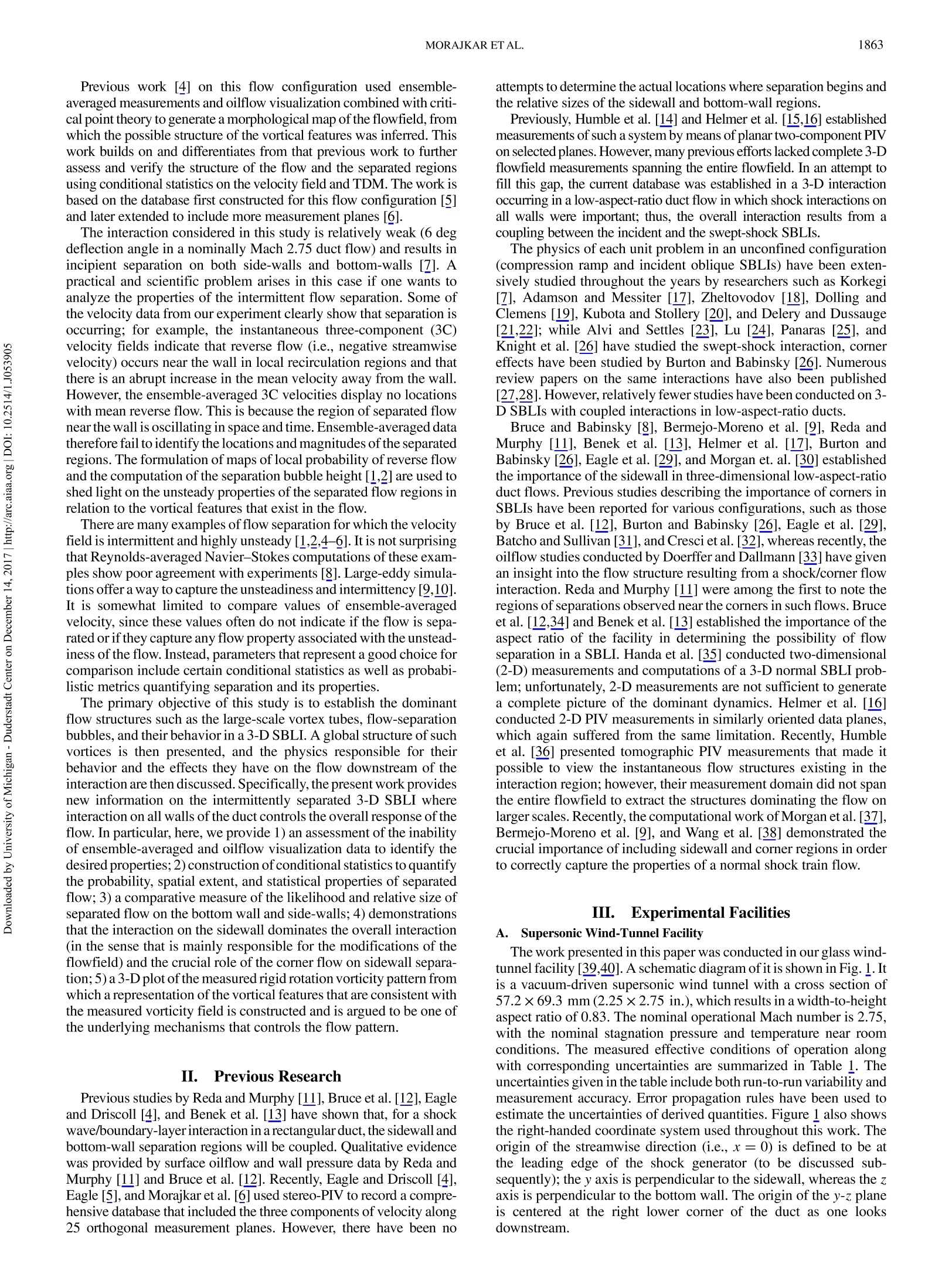
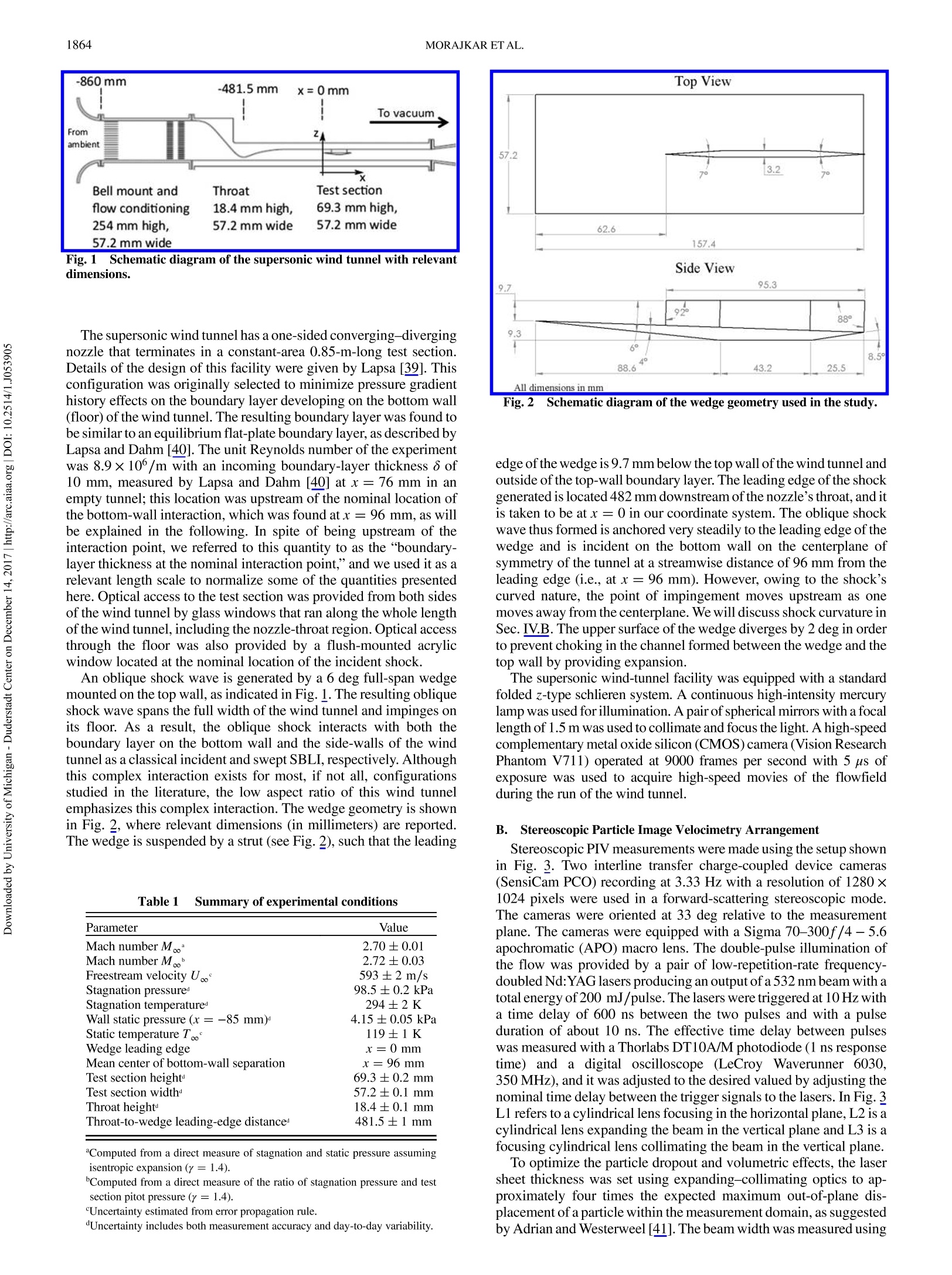

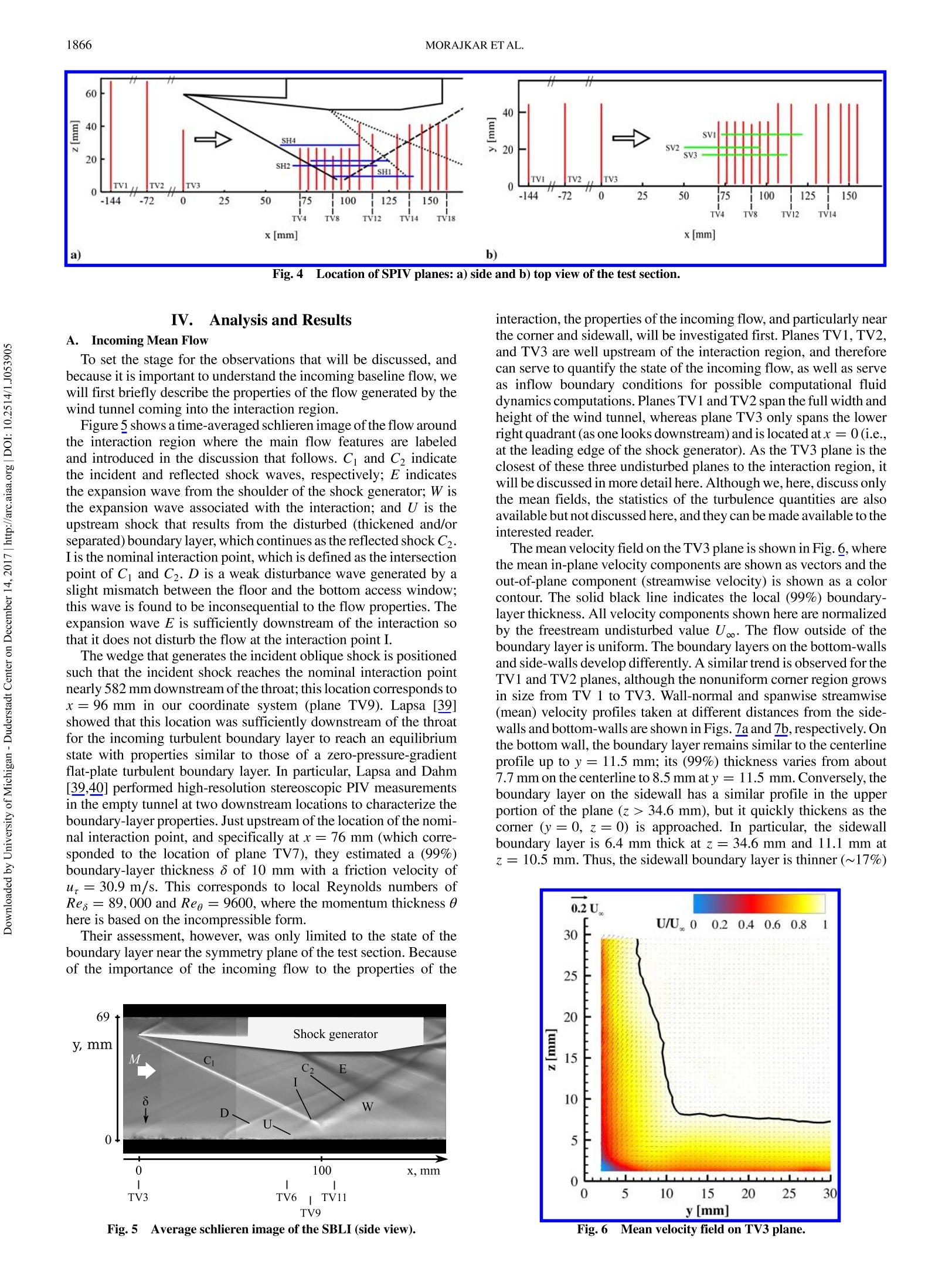
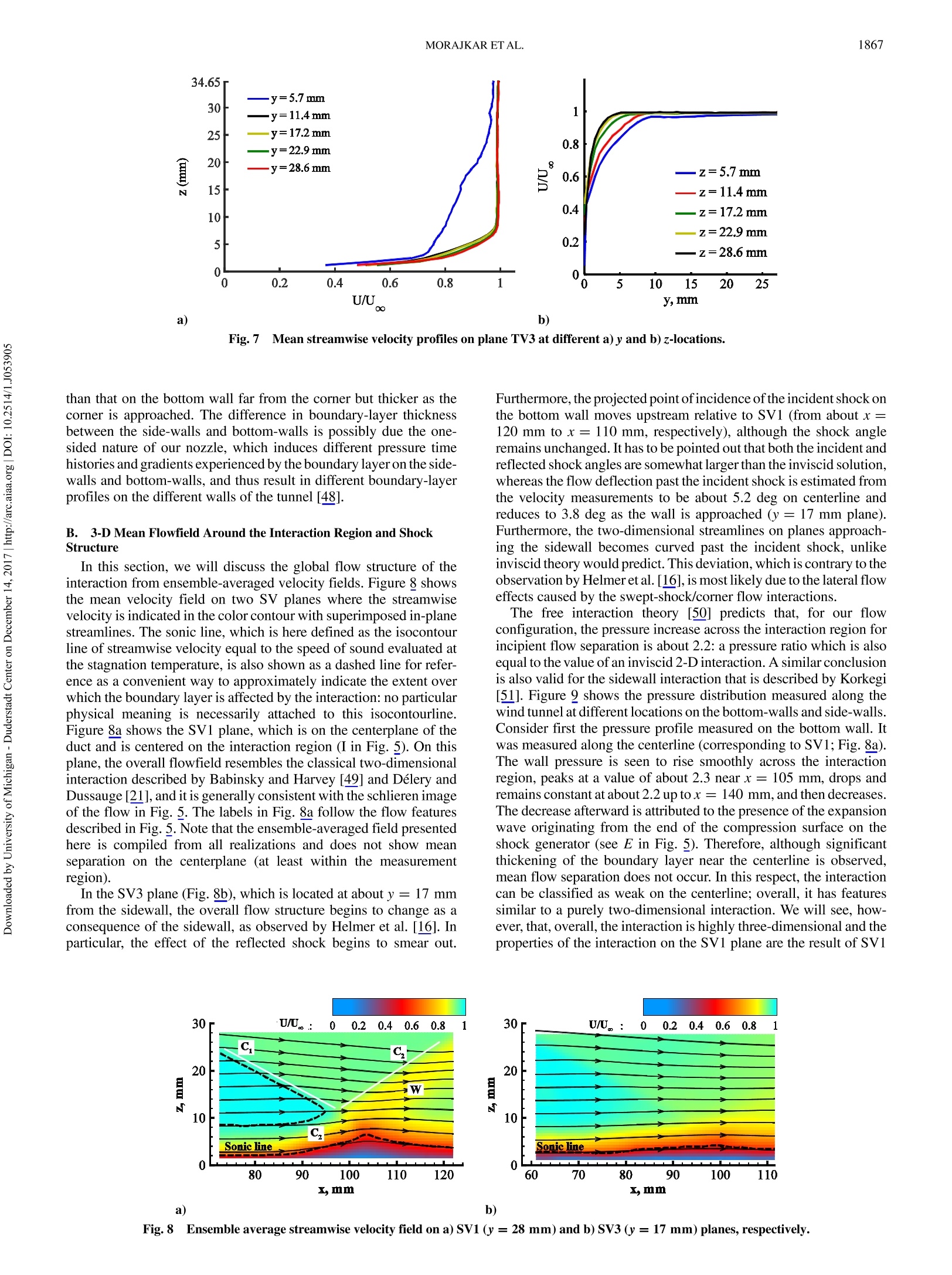
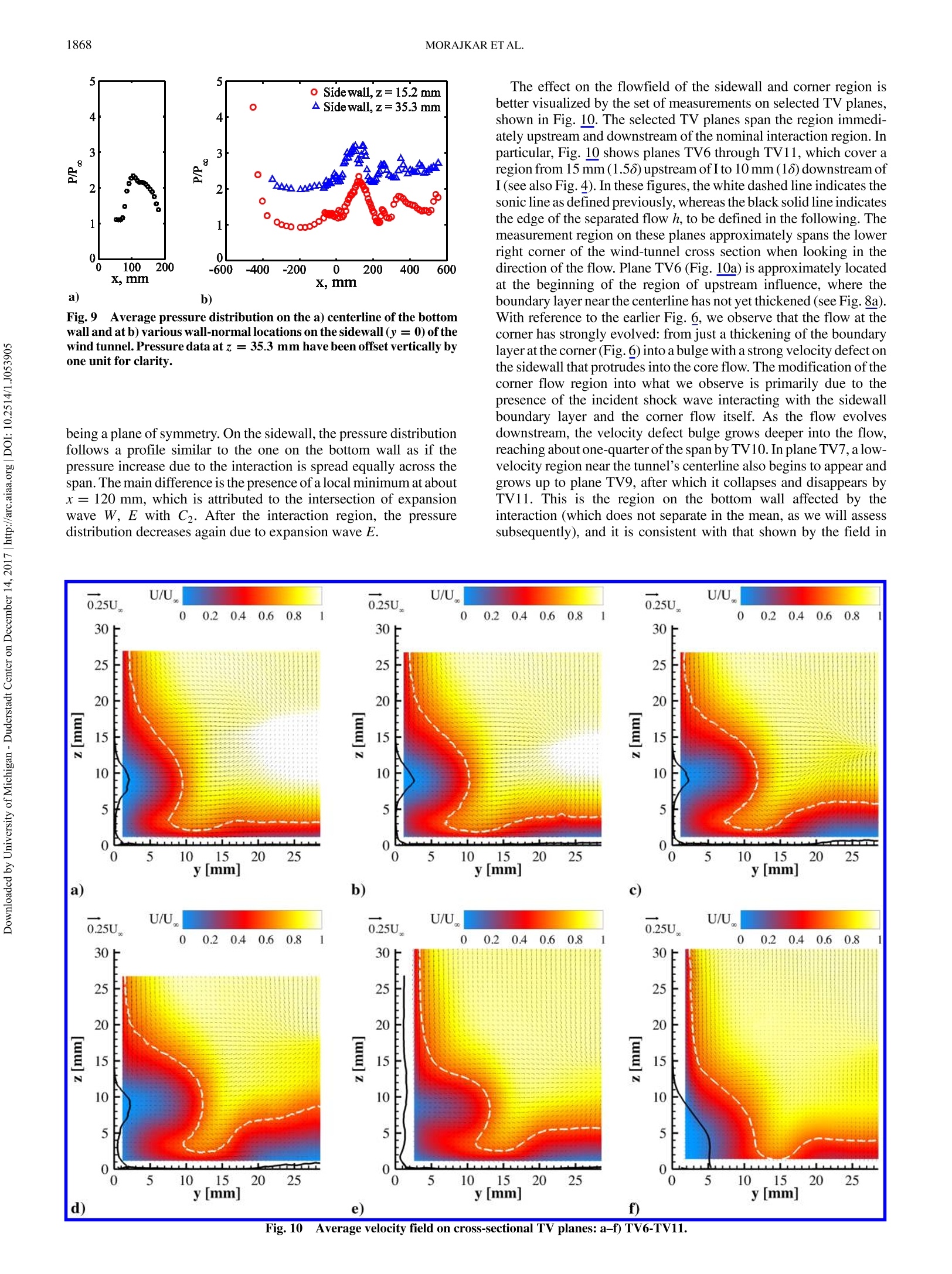
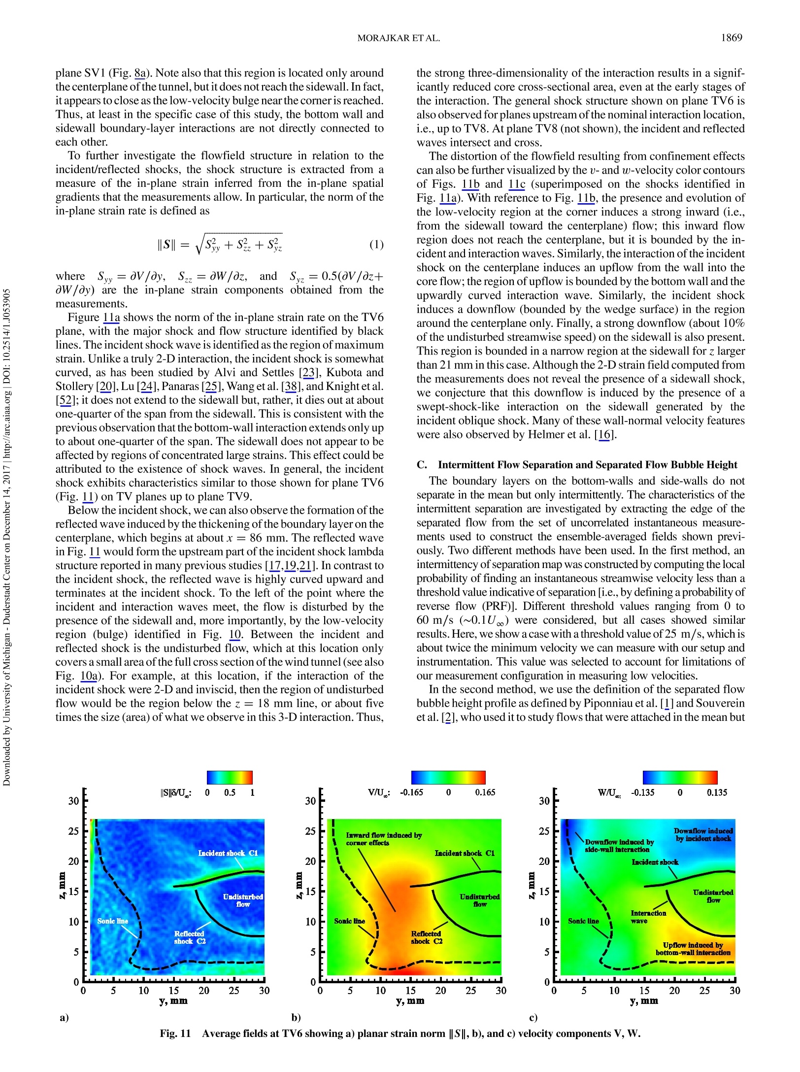
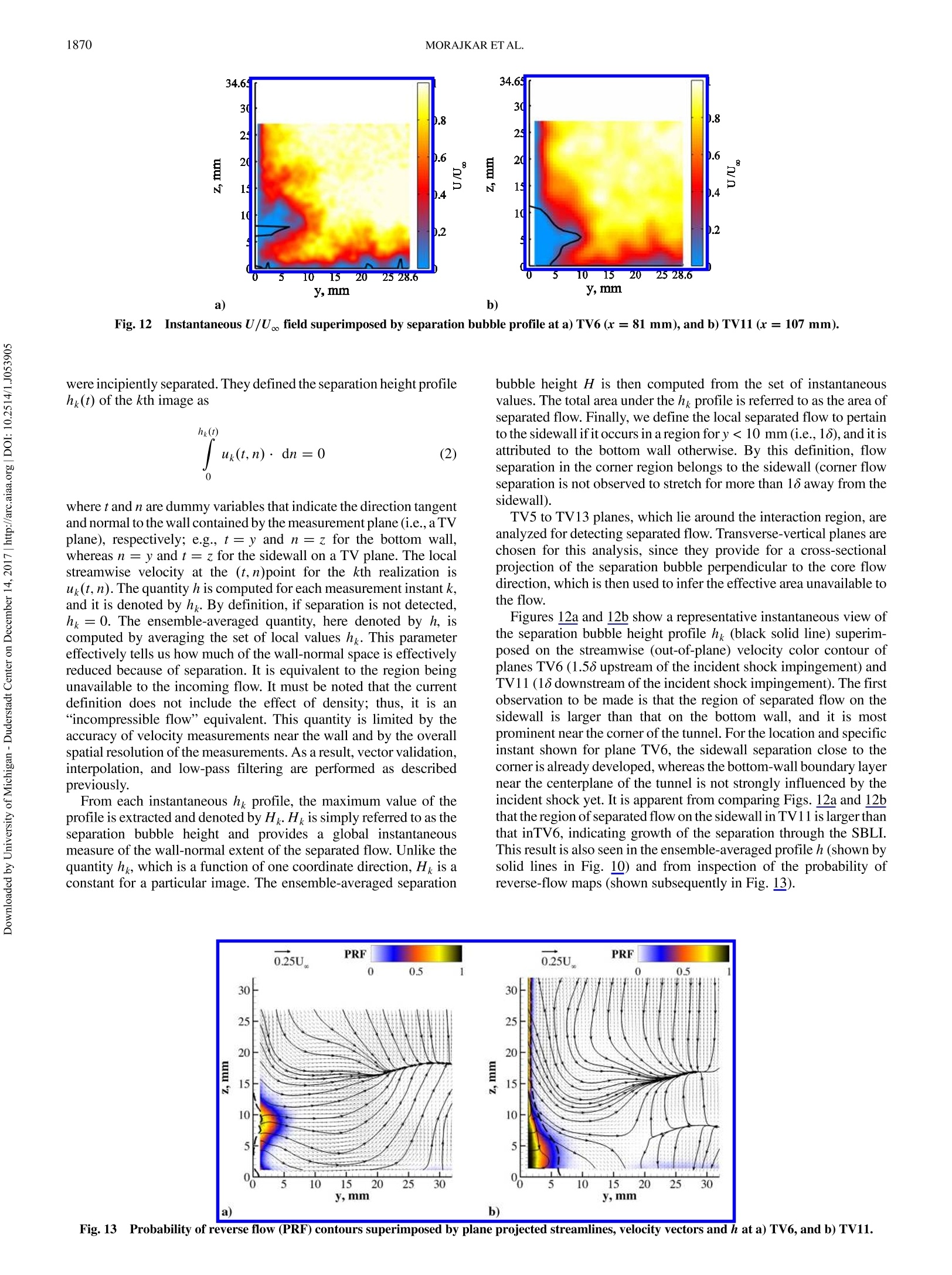
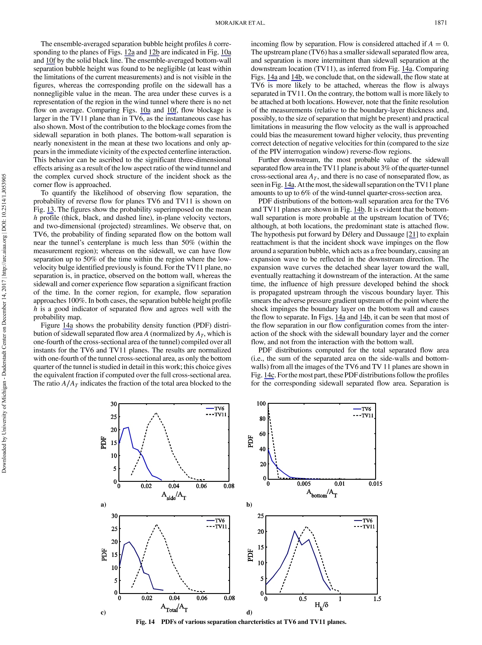
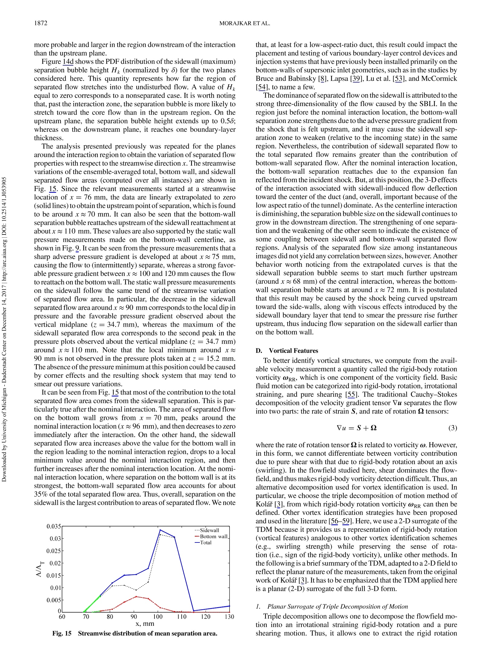
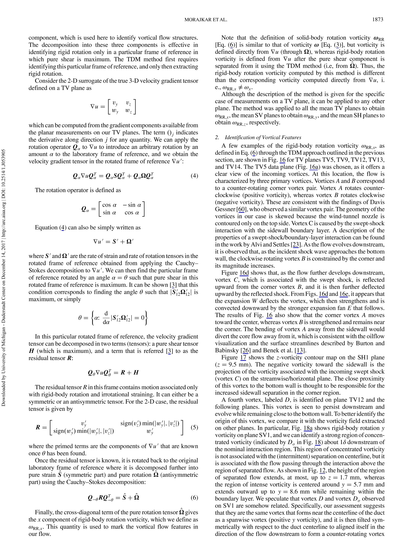
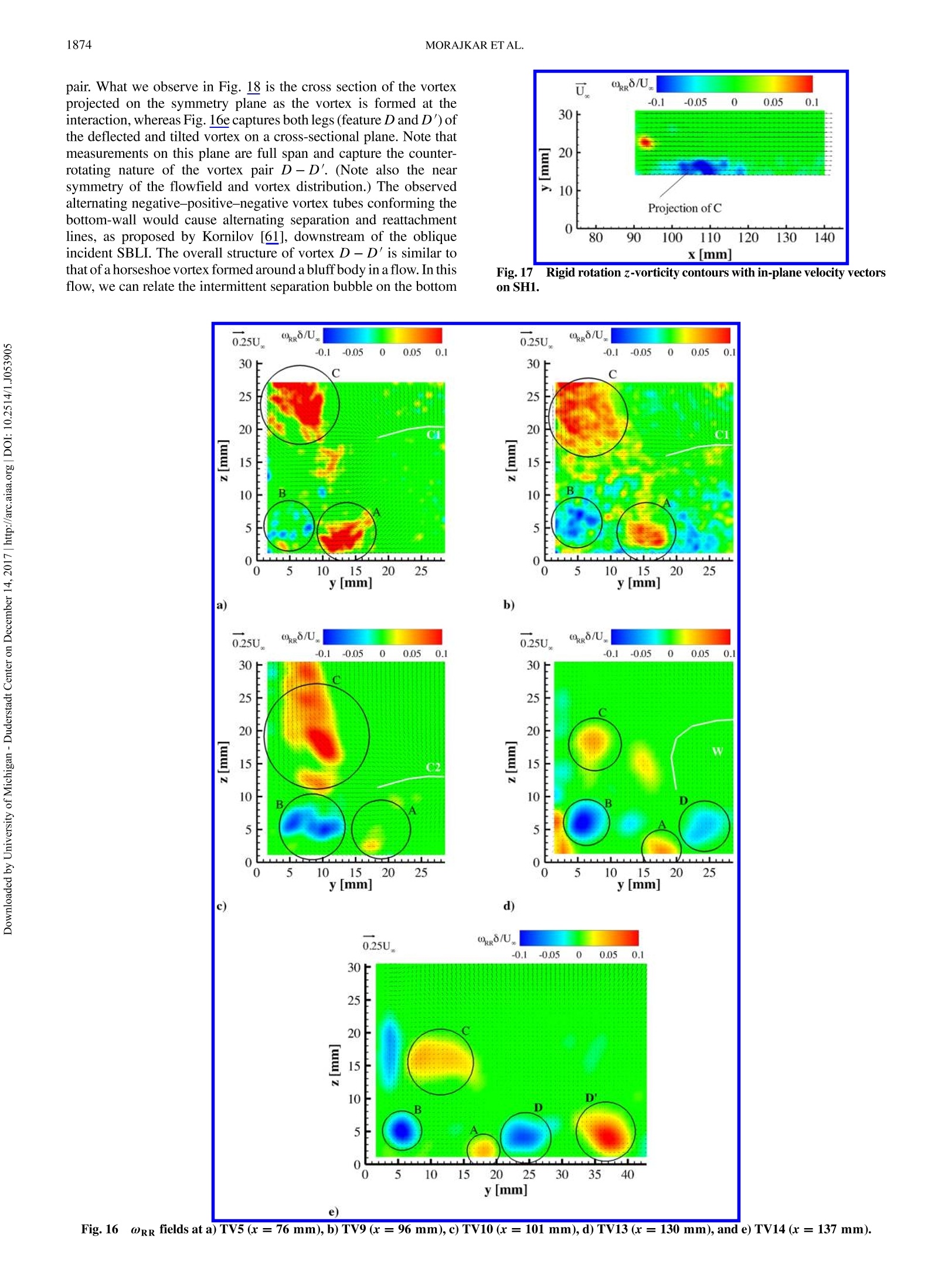
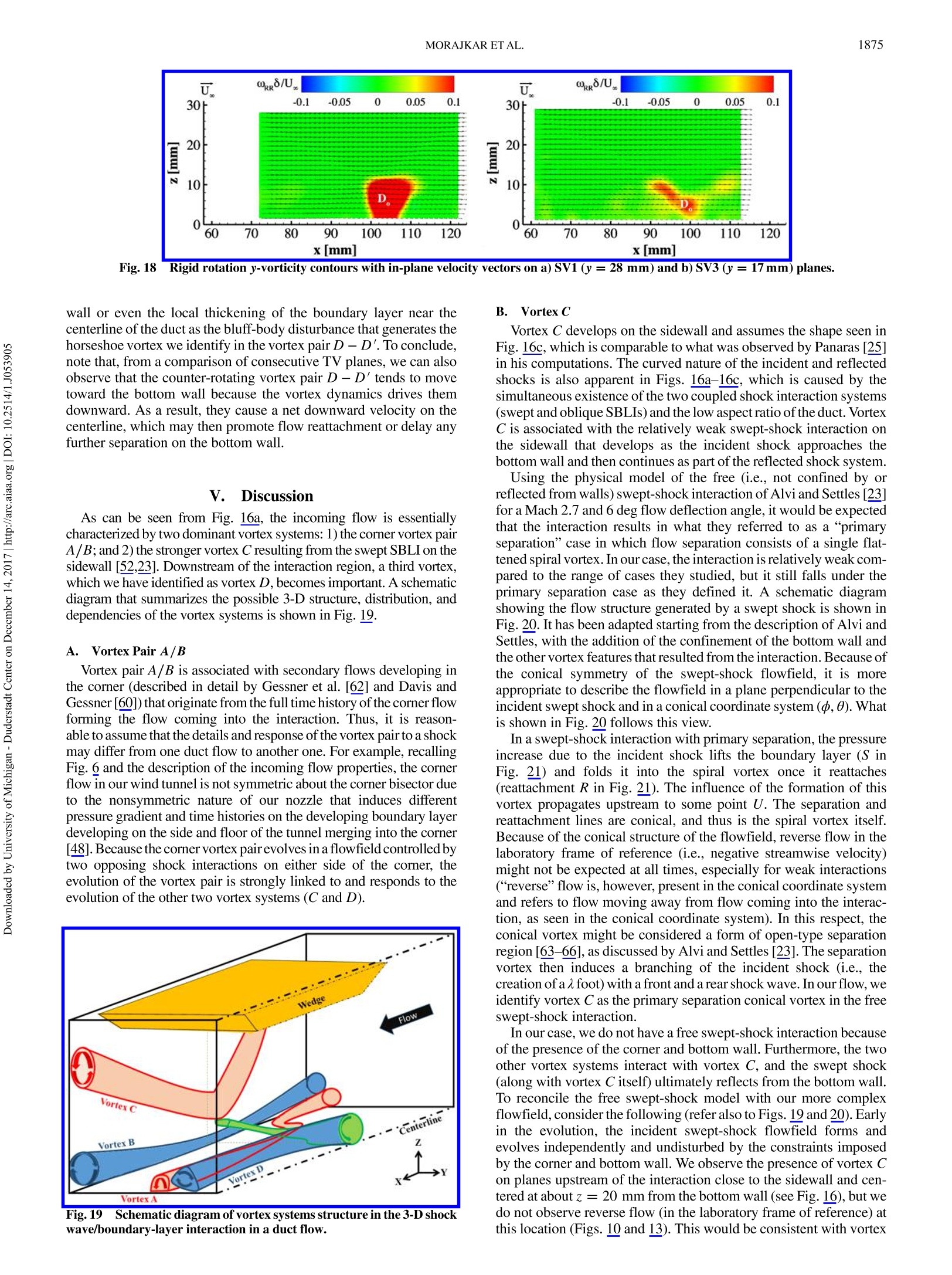

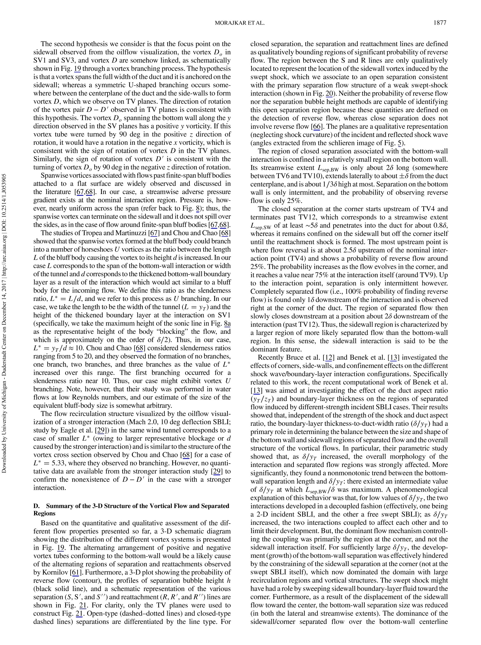

还剩17页未读,是否继续阅读?

产品配置单

北京欧兰科技发展有限公司为您提供《空气流场中间歇分离,涡结构检测方案(粒子图像测速)》,该方案主要用于其他中间歇分离,涡结构检测,参考标准--,《空气流场中间歇分离,涡结构检测方案(粒子图像测速)》用到的仪器有德国LaVision PIV/PLIF粒子成像测速场仪
推荐专场


相关方案
更多
该厂商其他方案
更多