


方案详情
文
采用一台Quantronix公司生产的Darwin Duo型双腔Nd:YLF激光器作光源。该激光器输出2 × 25 mJ 单脉冲能量,重复频率1 kHz。采用两台Photron Fastcam SA1 相机作成像器件。构成一套时间分辨高重复频率立体3维粒子成像测量系统。对NACA 0018翼型,加装整齐排列的锯齿状后缘时的流动的边界层特性和声学特性进行了测量。和未加装翼型的特性做比较,得到加装锯齿状后缘,可降低气动噪声的结论。
方案详情

Exp Fluids (2016) 57:182CrossMarkDOI 10.1007/s00348-016-2272-z 182Exp Fluids (2016) 57:182Page 2 of 22 TUDelft Delft University of Technology Boundary layer characterization and acoustic measurements of flow-alignedtrailing edge serrations Arce Leon, Carlos; Merino Martinez, Roberto; Ragni, Daniele; Avallone, Francesco; Snellen, Mirjam DOI 10.1007/s00348-016-2272-z Publication date2016 Document Version Final published version Published in Experiments in Fluids: experimental methods and their applications to fluid flow Citation (APA) Arce Leon, C., Merino Martinez, R., Ragni, D., Avallone, F., & Snellen, M. (2016). Boundary layercharacterization and acoustic measurements of flow-aligned trailing edge serrations. Experiments in Fluids:experimental methods and their applications to fluid flow, 57(182). DOI: 10.1007/s00348-016-2272-z Important note To cite this publication, please use the final published version (if applicable). Please check the document version above. Copyright Other than for strictly personal use, it is not permitted to download, forward or distribute the text or part of it, without the consentof the author(s) and/or copyright holder(s), unless the work is under an open content license such as Creative Commons. Takedown policy Please contact us and provide details if you believe this document breaches copyrights. We will remove access to the work immediately and investigate yourclaim. This work is downloaded from Delft University of Technology. For technical reasons the number of authors shown on this cover page is limited to a maximum of 10. Boundary layer characterization and acoustic measurementsof flow-aligned trailing edge serrations Carlos Arce Leon12@·Roberto Merino-Martinez²·Daniele Ragni?· Francesco Avallone’·Mirjam Snellen Received: 13 May 2016 / Revised: 19 October 2016 / Accepted: 20 October 2016 /Published online: 19 November 2016C The Author(s) 2016. This article is published with open access at Springerlink.com Abstract Trailing edge serrations designed to reduce air-foil self-noise are retrofitted on a NACA 0018 airfoil. Aninvestigation of the boundary layer flow statistical proper-ties is performed using time-resolved stereoscopic PIV.Three streamwise locations over the edge of the serrationsare compared. An analysis of the results indicates that,while there is no upstream effect, the flow experiencessignificant changes as it convects over the serrations andtoward its edges. Among the most important, a reducedshear stress and modifications of the turbulence spectrasuggest beneficial changes in the unsteady surface pres-sure that would result in a reduction of trailing edge noise.Microphone array measurements are additionally per-formed to confirm that noise reduction is indeed observedby the application of the chosen serration design over theunmodified airfoil. 1 Introduction Airfoil self-noise is known to be produced by different aer-oacoustic mechanisms, an identification and descriptionof which is available from Brooks et al. (1989). The noisecaused by the convection of turbulent eddies over the sharptrailing edge of an airfoil is called turbulent-boundary-layer trailing edge (TBL-TE) noise. This source of noise ( 区 Carlos Arce Leon ) ( caar@lmwindpower.com ) Aerodynamics and Acoustics Group,LM Wind Power R&D,J. Duikerweg 15-A, 1703 DH Heerhugowaard,The Netherlands 2 Faculty of Aerospace Engineering, Delft Universityof Technology, Kluyverweg 1, 2629 HS Delft,The Netherlands is dominating in several noise-regulated industrial applica-tions, such as wind turbines (Wagner et al. 1996; Pedersenet al. 2009), urging an investigation over its productionmechanisms and mitigation techniques. Theoretical formulations of TBL-TE noise for conven-tional straight trailing edges have been proposed using anumber of approaches. Examples of these can be foundin Amiet (1976), Chase (1972), Howe (1999) and Parchen(1998). An extension of the theory for variable trailing edgeshapes has in addition been formulated by Howe (1991).Based on this solution, variable trailing edge shapes havebeen found to reduce the efficiency at which TBL-TE noiseis produced. In particular, a serrated trailing edge, which isshaped as a series of sharp sawteeth, has been identified tobe particularly promising for this objective (Howe1991). While serrated trailing edges have been acousticallymeasured in wind tunnels, and their noise reduction effectshave been confirmed in Dassen et al. (1996), Moreau andDoolan (2013), Gruber et al. (2010) and Finez et al. (2011),Chong and Vathylakis (2015), the analytic prediction ofHowe (1991) yields too optimistic noise reduction levelscompared to the experimental observations (≈12 dB com-pared to 7 dB seen in wind tunnel measurements, over aselect frequency range). The analytical approach remainsnevertheless a valuable starting point for serrations design,as well as being a powerful tool for understanding the base-line mechanisms ofnoise reduction. It is worth noting thatLyu et al. (2015) has later provided an alternative approachto the Howe (1991) model that includes the hydrodynamicinteraction between adjacent serrations, obtaining resultsthat are in better agreement with the noise reduction lev-els observed in wind tunnel experiments. Azarpeyvandet al. (2013) has further developed Howe’s theory to coverother trailing edge geometries mixing combs and saw-tooth shapes, as well as sinusoidal variations over sawtooth baselines. These have been complemented by wind tunnelmeasurements in Gruber et al. (2013). The promising results have made serrations an attrac-tive option in the pursuit of reducing the noise from windturbine blades. Field measurements have been performed,confirming that noise reduction can be obtained in large-scale applications. Examples of these can be found in Oer-lemans et al. (2009) and Schepers et al. (2007). Severalindependent field tests have further been carried out byseveral industrial players, including LM Wind Power, withwhom a full-rotor overall sound pressure level reduction ofup to 3 dB has been obtained (private communication withJesper Madsen, Chief Engineer, Aerodynamics, LM WindPower). The research on serration-retrofitted airfoils is thuscritical in the pursuit of an improved and more reliabledesign, based on a scientific understanding of the underly-ing mechanisms of noise reduction of an unmodified airfoilby trailing edge serrations. Two potential factors have been proposed that drive thenoise reduction. The first is the modification of the flow andsurface pressure by the physical presence of the serrations(Jones et al.2010; Moreau and Doolan 2013; Chong andVathylakis 2015), and the second leans on a change in thescattering of the surface pressure by the modification of thetrailing edge geometry (Gruber 2012; Howe 1991). Despitethe two potential factors being assessed, their weight in thefinal noise reduction is still unknown. The solution of thisdichotomy remains critical, as the dominance of either canlead to different preferred optimization approaches for ser-ration design. In this paper, the approach used to addressthis duality focuses on a characterization of the unsteadyflow over the serration, of which the fluctuating pressureon the serration surface argued to be a direct consequence(Blake 2012). An understanding of the surface pressure fluctuations iscritical, as TBL-TE noise is the result of the scattering ofsurface pressure waves into acoustic pressure waves by thesharp edge, driven by the impedance discontinuity betweenthe wall and the freestream. Nevertheless, while numericalstudies such as those of Jones et al. (2010), Sandberg andJones (2011), Jones and Sandberg (2012) and Arina et al.(2012) have provided field velocity and pressure solutions,as well as unsteady surface pressure information, obtainingthe latter experimentally over serrations is difficult due tothe relatively large physical size of available transducerswith respect to the surface pressure structures, and to thephysical thickness of the serrations themselves. Workarounds have been implemented, for example inGruber (2012) and Chong and Vathylakis (2015), whereserrations have been cut into a flat plate placed at the lowerside of a wind tunnel nozzle. In their study, the instrumented side is under a turbulent boundary layer, while theopposite side, from which the measurement instruments protrude, remains in a quiescent state. Although promising,the method cannot be used in airfoil applications due to thedisturbances to the flow field that would be generated bythe protrusion of microphones or pressure transducers. On the other hand, advanced non-intrusive measure-ments techniques such as particle image velocimetry (PIV,Raffel et al. 2007) offer flow information with good tempo-ral and spatial resolution. Studies of the flow field aroundserrations have been performed previously in Finez et al.(2011), Arce Leon et al. (2016) and Avallone et al. (2016)using PIV. In Arce Leon et al. (2016), time-averaged resultsare used to quantify the level of mean flow modificationwhen serration-flow misalignment is prescribed by apply-ing an angle of attack to the airfoil or setting the serrationswith a flap angle. The results are considered in terms of theconditions assumed in Howe (1991), and ultimately con-cludes that misaligned serrations cause flow effects thatare not contemplated in the analytic solution, yet are notenough to explain the discrepancies between the predictedand observed reduction levels, and changes in the acousticspectra shape. Gruber (2012) investigated serrations without a detailedfocus on the level of flow misalignment. By using a highlycambered airfoil and serrations that protrude straight outfrom the angled trailing edge, it can be readily assumedthat the condition of flow alignment is not met. Flow visu-alization using smoke has confirmed this in Gruber et al.(2011). In the research of Moreau and Doolan (2013),the condition of flow alignment is more closely achievedby mounting serrations at the trailing edge of a flat plate.Nevertheless, the relatively large angle (12°) on the upperside of the flat plate as it narrows to form the sharp trail-ing edge does not help to ensure that equal flow conditionsover the upper and lower serration sides are obtained. Thestudy further focuses on the reduction of tonal noise com-ponents due mainly to vortex shedding. A more detailedresearch on serrations, where flow alignment is obtained,is therefore missing. With this baseline, a more realisticmeasurement of the boundary layer properties and theirchange along the serration surface can be achieved withoutthe effect of mean pressure differences between upper andlower surfaces. Having detailed hydrodynamic information, an imple-mentation of the so-called TNO-Blake prediction model forTBL-TE noise (Parchen 1998; Blake 2012) can further beapplied to qualitatively approximate changes to the surfacepressure. This model relies substantially on boundary layerinformation to approximate the noise emission by the scat-tering of the unsteady surface pressure at the trailing edge.Recent changes, provided by Stalnov et al. (2016), Bertag-nolio et al. (2014) and Kamruzzaman et al. (2012), havefurther shown improvements in predicting TBL-TE noiseby using modified boundary layer models and addressing Fig. 1 Airfoil and serrationdimensions and detail of themodular trailing edge (right) anisotropy in the boundary layer turbulence. Even thoughan extension ofthe method to a variable trailing edge shapehas not yet been proposed, the model itself can be used toproduce a qualitative analysis of the unsteady pressure overthe serration surface, and by extension, its scattering intonoise at the edge. The present study uses time-resolved stereoscopic PIV(Arroyo and Greated 1991) to obtain a 3-component planar vector field of the flow over thin trailing edge serrationsretrofitted on a NACA 0018 airfoil. No incidence has beenprescribed, in order to maintain a balance in the mean pres-sure between the serration sides, and a Reynolds numberof 263,000 is achieved in an open test section wind tunnel.The results are evaluated with a modified TNO-Blake equa-tion (Blake 2012) in order to qualitatively estimate stream-wise changes in the surface pressure along the length of theserrations. While a precise formulation for the noise emissionsbased on this equation is not possible, this research willexpose important differences in the estimated surface pres-sure between the straight edge airfoil and the serrated edgeairfoil. Additionally, streamwise locations of the latter arealso observed and discussed. In order to confirm that the adopted serrations areeffectively reducing far-field broadband noise generatedat the trailing edge, microphone array measurements arepresented. 2 Experimental set-up The experiments were conducted at the Delft University ofTechnology vertical wind tunnel (V-Tunnel). It has a con-traction ratio of around 60:1. The turbulence intensity hasbeen measured by Ghaemi et al. (2012) to be below 0.5%for a freestream velocity of 10 m/s at the exit of a cylindri-cal nozzle of 60 cm in diameter. In the present set-up, asquare nozzle of 40 ×40cm’ has been used with 20 m/sand higher freestream velocities. The turbulence intensityhas been verified by stereo PIV statistics to still stay at orbelow 1% at the present regime. A NACA 0018 airfoil, reference profile thickness foroutboard sections of state-of-the-art wind turbine blades, has been manufactured into an aluminum wing of chordC=20cm and span of 40 cm, equal to the test sectionwidth. The model has been installed in an ad hoc preparedopen test section with two long side plates to approximatethe two-dimensional flow condition over most of the wingspan. A modular trailing edge design in the airfoil allowsinserts to be retrofitted while keeping the surface free fromirregularities, as indicated in Fig.1 (right). The insert usedfor this set-up is a sawtooth trailing edge serration modelwith teeth of 2h= 4.0 cm length, or 0.2 C, and a=2.0 cmwidth,or 2= h. These dimensions follow the recommenda-tions for serration design of Gruber et al. (2011). In par-ticular, it is suggested that the length required to achieve anoise reduction must comply with 2h 8, for 8 the bound-ary layer thickness. In the present case 2h~ 48, as will bediscussed in Sect. 3.1. The serrations are of flat-plate type, made of laser-cutsteel, with a constant 1 mm thickness throughout the spanand length, equal to the nominal thickness of the unserratedairfoil trailing edge. At this thickness, they remain stiffwith respect to any flow-induced vibration. A schematic ofthe airfoil and serration dimensions is shown in Fig. 1. All measurements were conducted at o=0°angleof attack. A freestream velocity of 20 m/s was chosen forthe PIV measurements, resulting in a chord-based Reyn-olds number of 263,000. This velocity was selected as itis the highest with which time-resolved flow informationcan be gathered with the current high-speed PIV system.The acoustic measurements were conducted at speeds of30, 35 and 40 m/s. In this case, the higher velocities wereneeded in order to distinguish the trailing edge noise fromthe background noise, especially for the reduced levelsobtained when serrations were applied. The reconciliationbetween the PIV and acoustic measurement velocity differ-ences is addressed in Sect. 3.3. At the tested velocities, the boundary layer is forced toturbulent transition with randomly distributed roughnesselements. The trip tape was constructed by an appropri-ate density of dispersed carborundum elements of 0.6 mmnominal size, placed on a thin double-sided tape of 1 cmwidth, following guidelines outlined in Braslow et al.(1966). The tape, streamwise-centered at 0.2 C, spans the entirety of the airfoil. A stethoscope probe has been usedto verify that the boundary layer was tripped and that itremains turbulent downstream until the trailing edge. 2.1 Stereoscopic PIV Stereoscopic particle image velocimetry (Arroyo andGreated 1991) has been employed to obtain measurementsof the three velocity components in a plane aligned with theflow field. The flow was seeded with tracer particles froman evaporated glycol-based solution called SAFEX, pro-ducing liquid droplets of about 1 um. Illumination of theparticles was provided by a Quantronix Darwin Duo dou-ble cavity Nd:YLF laser, which has an energy of 2×25 mJat 1 kHz. Two high-speed Photron Fastcam SA1 cam-eras were used,equipped with 1024 x1024 px resolutionCMOS sensors with a pixel pitch of 20 um/px and a digitalresolution of 12 bit. Two Nikon NIKKOR macro-objectivelenses of 105-mm focal length at an aperture of fl5.6 wereused for the two cameras, respectively, mounted one per-pendicular to the flow field and the second one at a rela-tive angle of 35°with respect to the first. With an overalldistance of about 40 cm, the resulting magnification factoris about 0.40, entailing that the particle image on the sen-sor is limited by diffraction to about 10 pm (Meinhart andWereley 2003). To avoid the problem of peak-locking, potentially pre-sent for the available 20 um/px pixel pitch of the cameras,defocusing is applied to the raw images by slightly displac-ing the focus plane from the laser one (Westerweel 1997).The procedure allows keeping the particle images in therange between 1 and 1.5 px and to obtain a stochastic dis-tribution of round-off errors in the computed velocity field. Since the stereoscopic PIV method requires the camerasto be at an angle with respect to the measurement plane, aScheimpflug adaptor was used to correct the sensor meas-urement plane misalignment. The final field of view is thecalibrated and dewarped combination of the images of bothcameras. A resulting area of 2×5cm² was obtained bycropping the sensor to 512 ×1024 px, permitting the samefield of view for both time-resolved data and statistics, witha digital imaging resolution of about 20 px/mm. A samplecapture of one of the cameras is shown seen in Fig. 2. The triggering of the camera shutter and the firing of thelaser pulse was controlled by a LaVision HighSpeed Con-troller. The capture sequence command and data acquisi-tion, along with the data processing, was performed usingthe LaVision software DaVis8. Two acquisition set-upswere used to capture either time-resolved or uncorrelatedflow samples for averaging. Their respective configura-tions are detailed in the following two subsections. Forboth, a multi-pass stereo cross-correlation was applied witha final window size of 16× 16 px (or 0.8 ×0.8mm). The Fig. 2 Single camera capture of the airfoil trailing edge side (left),serrations and the tracer particles, illuminated by the laser. The flowgoes from left to right. An instantaneous vorticity field from the PIVcross-correlation result is overlaid for illustration purposes Fig.3 PIV set-up indicating the two camera locations and laser sheetformation with respect to the wind tunnel open test section and theairfoil. The circular-to-square nozzle exit conversion is shown forillustrative purposes adjacent windows were overlapped by 75% such that theflow is sampled with a spatial resolution of 0.8 mm and avector spacing of 0.2 mm. A view of the PIV set-up is shown in Fig. 3. The cam-eras are located on the side of the airfoil, one perpendic-ular to the laser sheet and another above it, as previouslymentioned. The laser is fired from the side and orientedperpendicular to the airfoil surface by means of a mirror. Itis formed into a sheet of about 1 mm thickness in the fieldof view region using optical lenses. The bottom part of thewind tunnel nozzle corresponds to the contraction from thetunnel circular exit of 60 cm to the 40 x 40 cm²test sectionnozzle exit, of which an approximate cutout is illustratedhere. The side plates for this set-up are made of Plexiglasto allow optical access for the cameras to the region ofinterest. For the serrated edge, three spanwise locations weremeasured at planes normal to the z axis. A schematic ofthese locations is shown in Fig. 4, along with the orienta-tion of the coordinate system and the location of its origin. Fig. 4 Wall-normal measurement plane locations over the serrationsurface. The y axis is positive out-of-plane The x axis is oriented parallel to the airfoil chord in thestreamwise direction and located at the serration medianline of the serration and its root. The z axis is oriented inthe spanwise direction, and the y axis is in the wall-normaldirection. An auxiliary definition for the orientation of the xand y axes will be given below in Sect. 3.1 for wall-normalmeasurements over the airfoil surface. This becomes neces-sary to correct for the difference in angle between the airfoil and the serration surfaces, and adhere to the definitionfor the boundary layer measurements. The measurementplanes are located spanwise in the serration-width normal-ized locations z/= 0, 0.25 and 0.5. 2.1.1 Acquisition ofthe uncorrelated dataset For simplicity, this set-up will be referred to as the time-averaged measurement for the remainder of the paper.The time separation between image pairs was chosen tobe At=50 us, yielding a particle image displacement ofapproximately 15 pixels in the freestream. A minimum dis-tance to the wall of around y 10 was achieved, limitedmainly by the finite digital resolution obtained with theset-up, as discussed in the results Sect. 3.1. An acquisitionfrequency of 250 Hz was chosen, ensuring that all vectorfields are uncorrelated at this flow speed. In total, 2000time instances were captured per case, for a total of 8s ofmeasurement time. 2.1.2 Time-resolved sample acquisition For the time-resolved sample acquisition, a continuousset of images is captured for which each individual imageserves as the cross-correlation pair for the following timeinstance. For this purpose, the repetition rate of each of thelaser cavities was set to 5000 Hz,while the pulse separation time was set to 100 ps. Being the pulse separation timehalf with respect to the repetition rate, the raw images canbeen re-shuffled in order to obtain a time-series of about10,100 particle images at 10,000 Hz. With this acquisitionfrequency, a particle displacement of around 24 px in thefreestream was achieved for the 20 m/s flow velocity (aboutdouble the one used for statistics). 2.1.3 Uncertainty analysis for the PIV method A linear propagation approach (Stern et al. 1999) was usedto estimate the typical measurement uncertainty. It was ver-ified a-posteriori using the statistical method introduced inWieneke (2015). Bias errors occurring to peak-locking (Westerweel 1997)happen when the particle diffraction spots are imaged withless than a pixel on the camera sensor. As mentioned in theexperimental set-up paragraph, the source is thus allevi-ated by following the technique proposed in Raffel et al.(2007), wherein it is suggested that a slight de-focusing ofthe images by the lens can bring the apparent particle sizeto above 1 px. A histogram of the particle displacement isprovided in Fig. 5 and shows the success of this approach,giving no evidence of peak-locking. Here, the decimalsof the measured velocity magnitudes, U -LU, where L.is the floor function, are binned into a histogram, whichwould show a large deviation toward one or more values,if a peak-locking error would dominate. The line plot rep-resents the cumulative distribution of the binned decimaloccurrences, showing a very close approximation to theideal result. Further, the finite spatial resolution of the resultingvelocity fields may limit the capture of flow structures.With the applied multi-pass cross-correlation algorithm,and the application of window deformation, the ampli-tude of the fluctuations is measured with less than 5%modulation, for window sizes smaller than 0.6 times the Measured Fig.5 Evaluation of the presence peak-locking error by means ofa decimal distribution histogram and a cumulative distribution ofbinned decimal counts characteristic structure length scale (Schrijer and Scarano2008). Having a window size of 0.8 ×0.8 mm , as speci-fied earlier, flow structures down to 1.2 mm can thus bemeasured within 95% accuracy. An iterative self-calibration procedure was applied to fur-ther improve the fitting of the captured planes from the ini-tial location-based calibration, which is based on a knownthree-dimensional target. The application of the two calibra-tion procedures helps alleviate further aspects such as thelens distortion. A final polynomial fitting used for the map-ping of the images is implemented within DaVis and iter-ated on the raw images, yielding a disparity vector of lessthan 0.10 px after self-calibration, considered satisfactory tocarry out the stereo cross-correlation (Raffel et al. 2007). The random errors in the measurement domain havebeen found to vary with less than 1% in the freestream andaround 3% in the inner boundary layer region. The methodused to approximate these numbers has been based on thework of Wieneke (2015). The mean velocity and velocity root-mean-square, orrms, of the fluctuations carry uncertainties that are depend-ent on the size of the statistical sample. For the presentcase, the error in the mean velocity reduces to 0.05% U,and on the rms to 2% Urms· 2.2 Microphone array Microphone arrays consist of a series of microphones dis-tributed in a particular configuration and are useful toolsfor sound source localization (Mueller 2002; Benesty et al.2008). These devices can be used for studying both station-ary sources, for example in wind tunnels (Mueller 2002;Sijtsma 2010), or moving ones, such as aircraft flyovers(Merino-Martinez et al. 2016a, b; Snellen et al. 2015). Acoustic images depicting the estimated locations andSound Pressure Level (SPL) of the sound sources can beobtained by applying a beamforming algorithm to theacoustic data of the array and considering a scan grid ofpotential sound sources. These algorithms are based onthe phase delays between the emission of the sound at theconsidered source location and the received signal at eachmicrophone in the array. There are several beamforming methods available, butthe most widely used for aeroacoustic experiments is thedelay-and-sum beamforming, also known as conventionalfrequency domain beamforming (Johnson and Dudgeon1993; Sijtsma 2010), due to its simplicity, robustness andlow computational demand. By evaluating a discrete Fou-rier transform of the data, an analysis of the frequencies ofinterest is possible. Moreover, this method provides con-tinuous results when applied to distributed sources (suchas trailing edge noise), unlike most deconvolution methodswhich show instead misleading spots (Dougherty 2014). For this experiment, microphone array measurementshave been employed to quantify the noise reduction capa-bilities of the adopted serration. An array with 64 micro-phones and of an effective diameter, D, of 0.9 m was used,arranged in a multi-arm logarithmic spiral configuration(Mueller 2002; Probsting et al. 2016), as shown in Fig. 6.The array was placed 1.26 m away from the airfoil in thedirection normal to the mean camber plane of the airfoil, asillustrated in Fig. 7. The center of the array was aligned inthe streamwise direction with the root of the serrations atthe trailing edge. The test section was modified from that described in thePIV set-up in order to have longer side plates, terminating0.7 m downstream of the airfoil trailing edge. Furthermore,the airfoil leading edge is separated 0.5 m from the noz-zle exit. These measures helped to separate the extraneousnoise sources coming from the nozzle and the downstream Fig.6 Microphone distribution of the array. Coordinates are shownin the airfoil system Fig. 7 Sideways view of the set-up used for the acoustic measure-ments. The microphone array can be seen on the left of the test sec-tion. The front wooden side plate is rendered semi-transparent to indi-cate the location of the airfoil edges of the side plates from the airfoil trailing edge noisesource. The sampling frequency used was 50 kHz, and theselected sound frequency range of interest extended from1 to 5kHz. For each measurement, a recording time of60 s was employed. The acoustic data was averaged usingtime blocks of 2048 samples (At=40.96 ms) for eachFourier transform and windowed using a Hanning weight-ing function with 50% data overlap. With these values, thefrequency resolution for the source maps is 24.41 Hz. Theaveraged cross-spectral matrix required for beamformingwas obtained after cross-correlating the microphones sig-nals. The expected error (Brandt 2011) in the estimate forthe cross-spectrum is, therefore: Considering a normal Gaussian distribution for the meas-urements (Brandt 2011), the spectral estimate 95% confi-dence interval is: With the normalized random error calculated in Eq.(1), weobtain: where Gxx and Gxx are the true and the measured values ofthe cross-spectrum,respectively. The rectangular scan grid used for beamforming cov-ered the expected area of noise generation, ranging fromz=-0.22 m to z=0.22 m in the spanwise direction andfrom x=-0.7m to x=0.3 m in the streamwise direc-tion, according to the axes defined in Fig. 4, with a distancebetween grid points of 1 mm. Therefore, the scan grid cov-ered the whole airfoil and went from the nozzle exit until0.3 m after the trailing edge using 441 x1001 grid points. The lower boundary of the minimum angular distance atwhich two different sources can be separated using an arrayof circular aperture of diameter D can be estimated usingthe Rayleigh criterion (Lord Rayleigh FRS 1879): For the current experimental set-up, the minimum angulardistance for the highest frequency considered in this anal-ysis (5kHz), considering c=340 m/s, is p=0.092 rad.Thus, the minimum resolvable distance, R, at a distancefrom the array r of 1.26m is R=rtanp~0.12 m. There-fore, the selected spacing between grid points is approxi-mately 120 times smaller than the Rayleigh’s limit distanceat that frequency. Because trailing edge noise is supposed to be a distrib-uted sound source, the source maps were integrated overan area extending from z=-0.1 m to z=0.1 m and fromx=-0.06m to x=0.06 m (see Fig.29). This section waschosen to minimize the contribution from extraneous soundsources, while still containing a representative part of thetrailing edge (Pagani et al. 2016). The beamforming resultsin that area were normalized by the value of the integral ofa simulated point source of unitary strength placed at thecenter of the area of integration, evaluated within the samespatial boundaries (Sijtsma 2010). This process was thenrepeated for each frequency of interest to obtain the acous-tic frequency spectra of the trailing edge. Each microphone was previously calibrated using a pis-tonphone which generates a 250 Hz signal of known ampli-tude. Moreover, the performance of the array itself wasassessed and calibrated by using tonal sound generated witha speaker at a known position emitting at several single fre-quencies: 500, 1000,2000,3000,4000 and 5000 Hz. TheSPLs at the center of the array were also measured with acalibrated TENMA 72-947 sound level meter. Therefore,the microphone array was calibrated in both source posi-tion and strength detection. The effect of the shear layer in the acoustic measure-ments (Amiet 1975) was neglected due to the small angle(<10°) between the center of the array and the scan area ofinterest and the considerably low flow velocities employedin this experiment (Salas and Moreau 2016). 3Results A study of the results, together with an analysis of thequantities relevant for the noise generation, is here pre-sented. First, a characterization of the boundary layer isshown based on the time-averaged PIV measurements.This is done in order to identify both the effect that the ser-rations have on the flow directly upstream of the trailingedge, and the mean flow and turbulence parameters pertain-ing to the flow as it convects over downstream locations ofthe serration edge. The statistical description of the flow field in terms ofaverage velocity and Reynolds stresses indicates whichregions, within the boundary layer, exhibit larger levels ofturbulence intensity. Nevertheless, the correlation betweena change in the latter and the pressure fluctuations at theobject surface remains complex. To study such a link, the results will then focus onthe elements of the TNO-Blake model based on resultsobtained from the time-resolved PIV measurements, withthe objective of providing a qualitative comparison betweenthe flow at three different locations over the serration edge, and the straight edge. This is done to estimate the levelof modification that the flow experiences and evaluate apotential correlation with the noise reduction mechanism ofthe serrations. Lastly, the results of the acoustic measurements arepresented with the purpose of confirming and quantifyingthe noise reduction effects that this serration design offerswhen retrofitted on the used airfoil profile 3.1 Mean flow characterization of the turbulentboundary layer In the present section, the mean flow and turbulence statis-tics of the boundary layer are introduced. Focus is placedon establishing whether there is a measurable effect of theserrations immediately upstream of x/2h= 0, and on theway the flow in the boundary layer evolves along the ser-ration surface until it encounters its edge at different down-stream locations. Time-averaged measurements are taken with stereo-scopic PIV. Data are presented in the wall-normal direc-tion at different streamwise locations over the surface ofthe airfoil and the serration tooth. Note that, to adhere tothe definition of the boundary layer, the wall-normal linesover the airfoil surface and over the serration surface arenot parallel. For simplicity, the defined coordinate systemwill also be rotated accordingly, as indicated in the sche-matic of Fig. 8, such that y always points in the local wall-normal direction, and u =u+u, is the local wall-parallelcomponent of U, where u and u are the time average andfluctuating parts of the flow according to the Reynoldsdecomposition. The streamwise locations are picked 1 mm (0.025x/2h)upstream of the respective trailing edge, mainly to avoidthe directional ambiguity carried by the vertex between theairfoil and the serration tooth at x/2h= 0. This choice oftranslation in xis kept in all locations for consistency. Forsimplicity, the x/2h=-0.025 will still be referred to as theairfoil trailing edge and written as x/2h=0 in the rest of Fig. 8 Schematic of the boundary layer over the airfoil (angled sur-. face on the left) and the serration surface this paper. The locations x/2h=-0.025,0.475 and 0.975,along the serration trailing edge, will be referred to as theserration trailing edge and noted as x/2h= 0, 0.5 and 1.0. To analyze the boundary thickness, the surface-paralleledge velocity, ue, is taken as the velocity at the wall-nor-mal location y at which the spanwise vorticity, integratedfrom the closest available wall-normal location, ymin tos wz(y) dy, sy8,-Jy.@z(tabilizes. This method offers an accu-rate way to determine the boundary layer edge by virtueof the values of ω being negligibly small beyond it (seeSpalart and Watmuff 1993; Balint et al. 1991). The estab-lishment of ue in this way is preferable over assuming thefreestream velocity from the wind tunnel pitot tube meas-urements, as small deviations (±1%) are expected in themean flow freestream velocity between different runs,causing variations in the boundary layer locations. First, wall-normal results at x/2h=0 are presentedfor the straight edge and the 3 spanwise locations for theserrated edge: z/1=0,0.25 and 0.5. The objective is toestablish whether the serration has any measurable effecton the flow close upstream to it. Figure 9 shows the resultsobtained for the mean streamwise velocity, u. Differencesalong the wall-normal profile between the straight edge andthe serration, or spanwise locations of the latter, are practi-cally absent. The resulting boundary layer thickness values are givenin Table 1 for the different serrated edge spanwise loca-tions and for the straight edge, along with the results from Fig. 9 Wall-normal boundary layer profiles of u/ue at x/2h=0 Table 1 Measures of boundary layer thickness at x/2h=0 Trailing edge z/ 899(mm) 8*(mm) 0 (mm) Serrated 0 8.9 2.1 1.2 Serrated 0.25 9.3 2.2 1.3 Serrated 0.5 9.2 2.2 1.3 Straight 一 9.4 2.1 1.3 XFOIL 1.7 1.0 Fig. 10 Non-dimensional boundary layer profile at x/2h=0. Thedashed lines show the law of the wall and log-law the XFOIL (Drela 1989) simulation on the latter. The val-ues found from the PIV measurements on the straight edgeairfoil show a good approximation to the ones reported byXFOIL. As expected from Fig. 9 and the discussed simi-larity of the u wall-normal profiles, the values of 899, 8*and 0 (respectively, the boundary layer thickness at 99%of the edge velocity, ue, the displacement thickness, andthe momentum thickness) are also similar for all measure-ments, with 899 having a variation range of ±0.25 mm, 8* of±0.05 mm, and 0 also of ±0.05 mm. In the remainder of thearticle, if not explicitly indicated, 8 will refer to 899. The non-dimensional boundary layer profile is shownin Fig. 10 for the resolved vector field above the wall,y+> 10. It shows a departure from the log-law expectedfrom a flat plate boundary layer measurement, and insteadfollows the trend expected for a boundary layer in anadverse pressure gradient (Nagano et al. 1998; Lee andSung 2008), which is the case at this location over the air-foil surface. The skin friction coefficient. defined asCr=u(0u/0y)y=o, where u is the fluid dynamic viscos-ity, is a guide to the general shape of the boundary layer.It will be discussed later (Sect. 3.2.2) that the intensityof the mean pressure at the surface is found to be espe-cially sensitive to the shear experienced in the bound-ary layer, for which C is an indicator. The direct calcu-lation of C is impossible due to the absence of flow dataclose enough to the wall. Instead, the results presented inFig. 10 use an estimation of Cf based on a best fit of thedata against the log-law. The value found that best col-lapses the data (allowing for an expected deviation due tothe adverse pressure gradient) is found to be approximatelyCr=1.5×10⁻². An XFOIL simulation of the same set-up yields a value of C=1.87×10⁻² at the same stream-wise location, x/2h=-0.025 (or x/C=-0.05). The Cfvalue of 1.5 x 10⁻² in the XFOIL simulation is reachedinstead slightly downstream at a streamwise location ofx/2h=-0.14 (or x/C=-0.028). This represents a small deviation of around 0.03 C or 0.11 2h. The approxima-tion of the friction coefficient is thus considered satisfac-tory and will be examined later to evaluate its downstreamevolution. The wall-normal profiles of urms and vms at x/h=0are presented in Figs. 11 and 12. Only slight differencesare observed between the different locations of the ser-rated edge and the straight edge. The urms shows highervalues, slightly above or around 0.09 ue, at locations nearthe surface, at around y/8=0.2-0.3 The values of urms rap-idly decline, reaching an asymptote of around 0.01 ue byy~ 1.18. Values of vrms show the same trend as urms, but with alower maxima of around 0.05ue. The maxima happen ataround the same wall-normal location as for urms, and thedecline is seen to reach minima slightly above that for urms,in this case being closer toy≈1.28. Having discussed the mean flow properties of the wall-normal data at the x/2h=0 location, it is established thatthe serrations have a negligible effect on the flow immedi-ately upstream. The same analysis will now be applied tothe 3 streamwise trailing edge locations of the serrations, atx/2h=0,0.5 and 1.0. The measured u is shown in Fig. 13. Contrary to whatwas discussed for x/2h =0 in Fig. 9, the velocity profilesseen here for the different cases vary significantly. The Fig. 11 Wall-normal profiles of ums/ueat x/2h=0 Fig. 12 Wall-normal profiles of vrms/ue at x/2h=0 Fig. 13 Wall-normal profiles of u/ue at different spanwise trailingedge locations of the serration and the straight edge straight edge case, and the serration at x/2h=0, are at thesame locations as presented before and are included here tofacilitate the comparison with the locations further down-stream. As the boundary layer develops, the u profile exhib-its an increase in velocity. Figure 14 provides evidence that the two downstreamlocations agree more closely with the log-law than the pre-viously discussed measurements at x/2h=0. A good fitis found between 20 < y+<100 for x/2h=0.5, andbetween 50 < y+<150 for x/2h=0. These two profilesalso fit closer to non-adverse pressure gradient conditions,from which the measurements at x/2h =0 deviate consid-erably, as was discussed above. The approximation of Cefor x/2h=0.5 yields a value of Cf=2.6× 10⁻², and forx/2h=1,Cf=3.3×10-2. Again, for both the serrated andstraight edge at x/2h=0, Cf was established earlier to be1.5×10-2. It can be concluded that the skin friction coefficientincreases for downstream locations of the serration edge,and is larger than that of the straight edged airfoil, approxi-mately doubling by the time the flow reaches the tip ofthe serration. This directly relates to an increase in the Fig. 14 Non-dimensional boundary layer profile measured at differ-ent spanwise trailing edge locations of the serration and the straightedge. The dashed lines show the law of the wall and log-law boundary layer shear observed near the wall. The veloc-ity shear is later reduced after y/8 ≈ 0.1,as confirmed bythe mean flow profiles in Fig. 13. This reduced shear in themiddle and upper boundary layer, thanks to the lower skinfriction of the lower boundary layer which has allowed alarger velocity compared to the same wall-normal loca-tions of the x/2h=0 measurements, spans a larger extentof the boundary layer. It will be shown later that, accord-ing to Eq. (4), this change ascribes to an expected benefi-cial change in the qualitative mean pressure values at thesurface. The measured boundary layer thickness parametersfor these trailing edge locations are shown in Table 2.The 899values appear to shrink downstream, becoming10% thinner when measured over the tip of the serra-tion at x/2h=1 than when done so over x/2h=0, butit is very similar between the former and x/2h=0.5.The values of 8* and 0 show only small differencesdownstream. The rms measurements of u' and v’ are shown inFigs. 15i and 16. For urms, the maxima decrease at trail-ing edge locations downstream ofx/2h=0, from aroundum/ue=0.095 to um/ue=0.085. The locations of themaxima of x/2h=1 are higher than for the rest of thelocations, and stand around y/8~0.4 instead of betweeny/8 ≈ 0.2 and 0.3. The lower values of urms for x/2h=1and 0.5 persist at the same wall-normal locations up Table 2 Measures of boundary layer thickness at the trailing edge ofthe specified spanwise locations Trailing edge z/2 x/2h 899(mm) 8*(mm) 0(mm) Serrated 0 1 8.3 1.1 0.8 Serrated 0.25 0.5 8.4 1.3 0.9 Serrated 0.5 0 9.2 2.2 1.3 Straight 0 9.4 2.2 1.3 Fig. 15 Wall-normal profiles of urms/ue at different spanwise trailingedge locations of the serration and the straight edge Fig.16 Wall-normal profiles of vrms/ue at different spanwise trailingedge locations of the serration and the straight edge toums/ue=0.02 compared to the serrated edge at x/2h=0and the straight edge. The measurement of vrms shows thetrailing edge location at x/2h=0.5 to have a larger rmsthan the rest of the presented locations, which is unex-pected based on the evolution of the boundary layer down-stream of the airfoil. 3.2 Turbulence statistics and qualitative analysisof surface pressure In order to establish the effect that the observed boundarylayer properties have on the surface pressure, the time-resolved PIV dataset is used here to characterize the differ-ent elements of the TNO-Blake surface pressure approxi-mation (Blake 2012), Here prefers to the fluid density, Aylvrefers to the wall-normal integral length scale taken over the flow compo-nent v, Ue refers to the wall-normal-dependent convectionvelocity magnitude,小Pwv(kx=w/Uc(),kz=0) refersto the wavenumber spectral density of the v flow compo-nent where k is the flow component-dependent wavenum-ber. It can be shown that only kx=w/Ue(y) contributes tothe radiation at frequency w (Bertagnolio et al. 2014). Ananalysis of the wall-normal and streamwise dependenceof these values will be given below and the results will besummarized in Sect. 3.2.5. The term Apz is the spanwisesurface pressure integral length scale and is relevant to geta final approximation to IIp. Unfortunately, as discussed inthe introduction, Aplz is technically impossible to quantifyin this case due to the unavailability of transducers thinenough for these serrations and is therefore left out of thisdiscussion. 3.2.1 Vertical integral length scale The vertical integral length scale results, shown in Fig. 17,are calculated as (Kamruzzaman and Lutz 2011) where is the correlation coefficient between the signal of v at thewall-normal location y, and that separated by 5in the wall-normal direction. The resulting Rw values for the serratedstreamwise location x/2h =1 are presented in Fig. 18 forreference. This results in a more complex prediction of theconstructive and destructive interference of the local scat-tered pressure waves along the edges. Overall, a wall-normal variation in Aylv of around3 mm is experienced for all cases, showing similar valuesbetween the streamwise measurement locations and anoverall increase in integral length scale at locations furtherfrom the wall, indicating an increase in turbulent struc-ture size as expected. A similar trend has been observed inKamruzzaman et al. (2009). There is a difference of val-ues between the cases along the same wall-normal loca-tion of no more than 0.5 mm, with the downstream location Fig. 17 Wall-normal values of Ayln Fig.18 Values of Ry for the serrated-case streamwise locationx/2h=1 initially showing lower values, and exhibiting a crossoverat y/8=0.6. The x/2h=0.5 location follows the upstreamlocation, either serrated or unserrated, more closely. Thissimilarity suggests that streamwise surface pressure varia-tions are weakly driven by this factor. 3.2.2 Convection velocity and mean velocity shear A wide variety of methods have been proposed to approx-imate the convection velocity, a good summary of whichis given in Renard and Deck (2015). In the present study,a spectral approach is taken based on Romano (1995) andused in Chong and Vathylakis (2015) to obtain the surface pressure convection velocity. It is obtained using thestreamwise cross-spectral density results and evaluating theslope of the phase spectrum over a two-point measurementseparation 5x, as where = arctan Im(Pu|12)Re(Pu12) and Pu|12 thestreamwise velocity component cross-spectrall(densitybetween streamwise locations x and x2=x1+5x. Tra-ditionally, it has been troublesome to obtain the velocityinformation at x2 since velocity probes located at xj disturbthe flow downstream. Since a non-intrusive measurementtechnique is adopted in the current study, a wide range of5is attainable, allowing a deeper evaluation of its depend-ence on o. Since 5 is wall-parallel, the streamwise componentof the convection velocity, uc, is evaluated instead of theconvection velocity magnitude, Uc. Since at the chosenlocations the wall-parallel component is largely domi-nant, the wall-normal and spanwise component contribu-tions to the convection velocity are considered negligible,and uc →Uc. Though for the sake of rigorousness, uc isindicated. The phase,中=(y,f,5x) is dependent on the stream-wise location, the frequency and the two-point measure-ment separation. Having a frequency dependence suggeststhat turbulent structures of different size might convect atdifferent velocities if df/do is not constant. It has never-theless been previously observed that in similar applications the relation between convection velocity and frequency appears to be negligible (Stalnov et al. 2016; Chongand Vathylakis 2015). This is confirmed in Fig. 19, whichshows a measure of for x/2h=1 and y/8=0.9, andwhere it is evident that p(y/8=0.9,f,5x) varies linearlyover f, with a slope that increases with larger 5. Only onecase is presented for conciseness, but the linearity ofd withrespect to the measured range of fhas been separately con-firmed for other streamwise and wall-normal locations. Fig. 19 Contours of 中 (left) as a function of frequency and 5x. A lineplot representation (right) is shown the linear nature of d. Measure-ment taken at x/2h=1and y/8=0.9 Being the result of an arctangent, the phase result var-ies as -刀<中≤n. A selective procedure has been appliedto remove the discontinuities in d over the presented fre-quency range. The signal coherence is seen to break downfirst at higher frequencies, and more rapidly for locationsnearer the wall and for smaller 5. Once this has happened,naturally the value of o becomes erratic and affects the cal-culation of uc by means of its slope. To account for this andkeep an accurate calculation of df/do, a procedure wasapplied by which the values of f() are linearly interpo-lated starting at f=0 until the coefficient of determina-tion drops below 0.97. The slope is then calculated fromthe result of the linear interpolation. Cases for which thecoherence was so poor that not enough samples over fwereemployable (<25% of those available) were discarded. The resulting convectionvelocity, calculated fromEq. (7), is shown in Fig. 20. The marker locations representthe mean of df/ do for the different values of tested. Thestandard deviation of the sample per wall-normal locationis represented by the gray region around the mean location. The dashed line represents the mean convection veloc-ity variation over the boundary layer, fitted with least-squares to the boundary layer log-law equation. The con-vection velocity is seen to depart slightly from the log-lawfit, fact which is highlighted in the left-most plot withhorizontal arrows, scaled with the magnitude of the differ-ence between the two values. This difference has a nega-tive maximum at around y/8=0.3 and a small positiveone at around y/8=0.7, becoming negative again at theuppermost region of the boundary layer. A similar behav-ior is replicated for the rest of the locations. Having estab-lished the presented uc as the mean over a wide range ofeddy sizes and events occurring throughout the boundarylayer, this departure from the log-law fit might suggest thata tendency for ejection events is experienced at aroundy/8=0.3, and of sweep events for y/8= 0.7, a discussionof which is presented in Romano (1995), Krogstad et al.(1998) and Ghaemi and Scarano (2013), and is expandedhere in Sect. 3.2.3. Fig. 21 Comparison of the convection velocity for the straight edgeand the streamwise measurement locations of the serrated case The mean flow profile, u, is indicated as a solid line inthe plots. The convection velocity is greater than u below acertain crossover point in the boundary layer. This crosso-ver is located at y/8=0.8 over x/2h=0 for both the ser-rated and straight edge cases, and around y/8=0.7 fur-ther downstream at x/2h=1. A similar trend of uc > uhas been observed in Atkinson et al. (2015) for a turbulentboundary layer over a flat plate, and Buxton and Gana-pathisubramani (2011) for a turbulent mixing layer. Thedegree of difference seen here is larger than that observedby Atkinson et al. (2015) and may be attributed to condi-tional differences between the two cases, possibly drivenby the adverse pressure gradient in the present one. Thisassumption is supported by the closer match in the down-stream location, where, as it was previously discussed, theboundary layer shows a better fit to the log-law. A direct comparison of the convection velocity for themeasured streamwise locations for the serrated edge andthat of the straight edge is presented in Fig. 21. It can beseen that the trend follows the one observed for the meanvelocity in Sect. 3.1, where the velocity near the wallexhibits an increasing as it moves downstream. The square of the mean velocity vertical shear factor ofEq. (4) is presented in Fig. 22, where the most downstreammeasurement location x/2h=1 exhibits the lowest valuesthroughout the boundary layer, followed by x/2h =0.5. A Fig.22 The square of the vertical shear of the mean velocity Fig. 23 The [v/uc]2 factor of Eq. (4) decrease of about 1s-2 in the maximum value is observedmoving downstream between the different measurementstations. The last remaining velocity-dependent factor in Eq. (4)is [v/uc], which is presented in Fig. 23. A significant dif-ference is observed between the measurements at x/2h =Oand the other streamwise locations. This is due to the wall-parallel flow at the location x/2h=0 encountering eitherthe surface of the serrations at approximately an angle ofl1°or the flow convecting from the opposite side of the air-foil (with a similar effect). This interaction causes the flowto gain upward momentum relative to the direction paral-lel to the airfoil surface, increasing the value of v. At thedownstream measurement locations, the flow at the edge Fig. 24 Wall-normal profiles of -u’v' at trailing edge locations remains instead relatively invariant in the v component, andthus the value of [v/uc]2 becomes driven by the denomina-tor, which is also several times larger than v. The measure-ment of this factor at x/2h=1 is less than half than that ofthe measurement at x/2h=0.5. As expected, at x/2h=0the measurement is similar for both the serrated and unser-rated cases. 3.2.3 Reynolds stresses, and sweep and ejection events The Reynolds stress, evaluated from a quadrant analysiscan give valuable information on turbulent structures thatconvect in the boundary layer. This information is also rel-evant as it may provide further understanding of surfacepressure peak events. In Chong and Vathylakis (2015), arelational approach between simultaneous pressure peakmeasurements on the surface is made along with turbu-lence fluctuation measurements in the boundary layer. Con-clusions in their observations indicate that, near the wall,events occurring in the IV quadrant are strongly correlatedto surface pressure peaks, and at regions further away fromit (near or beyond 8) the II quadrant events appear to contribute more. Separately, Ghaemi and Scarano (2013) findthat sweep events are correlated with positive pressurepeaks on the surface, and conversely, ejection events arecorrelated with negative pressure peaks. In a quadrant plot,the II quadrant is associated with ejection events and the IVquadrant to sweep events. For the purpose of evaluating the Reynolds stress vari-ation over the boundary layer, Fig. 24 shows the values of-u'v for the measured locations. The Reynolds stress val-ues for all streamwise locations reduce quite well to zeroat the measured y/8 location. The downstream serrationlocations at z/2=0 and 0.25 show a noticeably differentbehavior than for x/2h=0, exhibiting much lower valuesat their maxima, reaching about -u’v/u~3x10-, orabout two-thirds of that which is measured at x/2h =0. Asimilar observation has been made in Gruber (2012). In order to inspect the correlation of the velocity com-ponent fluctuations and perform a relational analysis to theexpected surface pressure events, a series of quadrant anal-ysis plots are shown in Fig. 25. Kernel density estimation(kde) contours for the entire time series are shown to moreclearly indicate the relational trends observed between thetwo component fluctuations over the four quadrants. Thehyperbola lines |uv|=-6u'v are presented, above whichare u’v events that are 6 times larger than the mean Reyn-olds shear stress (Kim et al. 1987;Lu and Willmarth 1973).The choice of the factor 6 is made to match that of Chongand Vathylakis (2015). In order to avoid overpopulating theplots, only events occurring outside of the -6u’vlimit areshown. The measurements over the straight edge are omit-ted for brevity, but are separately confirmed to be very sim-ilar to the measurements of the serrated case at x/2h=0. As is expected from the observations made in Fig. 24,away from the wall, at y/8=0.9, the magnitude of both u’and vis reduced. The events are also less correlated,indi-cated by the kde exhibiting a more circular footprint. At y/8=0.6 and below, the fluctuation componentsshow an anticorrelation between u' and v, indicated by anelongated kernel density distribution toward the II and IVquadrants. A larger range in the u direction is present, evi-denced by the kde being generally more slanted toward theuaxis. This pattern was also observed in Chong and Vathy-lakis (2015) and is supported by the larger urms magnitudeobserved above. There is additionally a marked existenceof events having a magnitude bias toward the II quadrant.Most events are nevertheless seen clustered in low valuesat the IV quadrant, as suggested by the location of the kdepeak. The fluctuations at y/8=0.3 remain more evenly con-centrated between quadrants II and IV, both in the locationof the kde peak and in its distribution. A slightly largerrange for u and vis exhibited. This is expected,as this isthe rough location where the rms maxima were observed inSect. 3.1, as well as from theobservations made of Fig. 24. The measurements nearest to the wall show slightlydecreased activity with respect to the mid-boundary layerlocations, especially in the wall-normal direction. This isagain expected from the observed rms results discussedbefore. A slight shift in the most-likely event location forx/2h =0.5 is observed, indicated by a bias in the kde peaktoward the II quadrant. At x/2h=1, this behavior is alsopresent but more moderate, and at x/2h=0, the peakremains instead centered at the origin. To simplify the observation of high-intensity events,Fig. 26 is provided, showing the percentage of the totalevents that comply with |uv|> -6u’v. In the currentresults, such events are present for all wall-normal loca-tions, but at y/8 > 0.6 , they are significantly biased toward the II quadrant, thus contributing to both high and lowpressure peaks at the surface. Closer to the wall, eventsare more evenly distributed between quadrants II and IV.Overall, there is a decrease in high-intensity events by upto around 2% moving downstream, which is beneficial fornoise reduction as it indicates the convection of less intensesurface pressure events at locations close to most of the ser-ration edge. This further implies that each location of theserration edge will contribute differently to noise reduction. In relation to the observed variance in the convec-tion velocity as shown in Fig. 20, the measurements aty/8=0.6 indicate that most events happen in the IV quad-rant, suggesting a larger number of sweep events (althoughevents are of lower intensity than events in the II quad-rant). This goes in line with the higher convection velocityobserved at around this height with respect to the log-law behavior. At around y/8=0.3, where the convection veloc-ity is lower than the log-law fit, the peak of the kde is wellcentered, indicating no event bias to either the II or IVquadrants. This is also true for the predominance of high-intensity events, which are also well distributed betweenthe II and IV quadrants. This symmetry inhibits an expla-nation of the observed convection velocity anomaly basedon the Reynolds shear measurements, requiring furtherinvestigation. 3.2.4 Turbulent flow spectra The final factor of Eq. (4) that is evaluated is the wavenum-ber auto-spectra. To evaluate the results, the frequency-dependent auto-spectra is provided in Fig.27 for both thestreamwise and wall-normal components. As observed Fig. 26 Percentage of eventswith |u'v|> -6u'v'occurringat each quadrant, for the differ-ent streamwise and wall-normallocations Fig. 27 The flow frequency-dependent auto-spectra of thewall-parallel component (left)and wall-normal component(right) at two wall-normallocations in the quadrant analysis above, the fluctuations over uhave a larger range, behavior which is reflected here, evi-denced by the larger energy of Puu compared to Pwy, whichis about 7 dB higher at the lowest frequencies presented. Both spectra follow the Kolmogorov -5/3 decay well untilhigher frequencies are reached. This is expected because oflimitations in the temporal resolution achieved by the PIVsignal-to-noise ratio between the instantaneous flow fields, Fig. 28 The flow wavenumber-dependent pre-multipliedauto-spectra of the wall-normalcomponent at four wall-normallocations y/8=0.60 ku 1/m ×102 which settles the maximum measurable frequency to about3/4 of the Nyquist frequency (Ghaemi and Scarano 2013).It appears to be more sensitive at lower boundary layerlocation presented,y/8=0.2, reaching a plateau at aroundf=3kHz for Puu. Overall, the results between the stream-wise cases are very similar. The most downstream locationdoes present lower energies in frequencies below 1 kHz forboth components, with Dw showing up to a 3 dB loss. The pre-multiplied wavenumber spectra are presentedin Fig. 28. Large overall level differences are seen betweenthe different wall-normal locations, reducing greatly forregions in the upper boundary layer. All the streamwiselocations exhibit peaks located close to ku~100 m.As expected from the frequency-dependent auto-spectraas shown in Fig. 28, the downstream location of the serrated edge shows lower levels, especially evident ataround y/8=0.4 and below for wavenumbers underku~200 m-. The ku location of the peak for the down-stream measurement appears to suffer a slight increase toaround 150 m-. A variation in the wavenumber suggestschanges in the intensity and spectral shape of the acousticemissions due to modifications in the turbulent structuresize and convection velocity. In the present case, the mostcontributing change appears to be in the intensity, withsmall variations in ke across the serration edge. 3.2.5 Summary of the flow parameter observations The different elements of Eq. 4 that are attainable from thehydrodynamic measurements have been considered in theprevious sections. Observations clearly indicate that the flow in the boundary layer changes as it convects past thedifferent edge locations of the serration. In summary, the following findings have been discussed: e tthe overall thickness of the boundary layer is reduced asthe flow evolves beyond the adverse pressure gradientthat is present between the end of the airfoil and the ser-ration surface. the vertical integral length remains similar along theboundary layer height between downstream locations, e tthe convection and mean velocity suffer changes,mostly seen below y/8=0.4, with downstream loca-tions exhibiting higher velocity, ● the shear is reduced downstream as a consequence ofthis. the factor v/ue becomes hard to evaluate, given the rela-tively large downward motion of the flow with respectto the boundary layer line at x/2h=0, but the down-stream location x/2h =1 shows slightly reduced levelswith comparison to x/2h =0.5, the quadrant analysis reveals the presence of turbulentstructures in the boundary layer that lead to high pres-sure peaks on the surface, but suggests a reduction ofthese events downstream. e ttrhe auto-spectra of the flow indicate that below a certainfrequency the downstream location over the serration tipexhibits less energy than the upstream location for boththe serrated case and the straight edge case, peaks in the: wavenumber auto-spectra arepresentaround 100 m-, with a slight increase seen for the tiplocation near the surface to about 150m-. Table 3 Boundary layer integrated values for the different elements of Eq. (4) Tailing edge x/2h Aylw(mm) uc (m/s) (ou/ay)²(s-2) /u×10-2 Product Straight 0.0 23.3 6.6 15.1 2.1 2.3 Serrated 0.0 23.8 6.7 14.6 1.3 2.3 Serrated 0.5 21.6 6.0 10.1 0.29 1.3 Serrated 1.0 19.2 5.8 7.4 0.06 0.8 a Disregarding v/u Fig. 29 Acoustic source mapsobtained for the airfoil with thestraight edge (top) and with theserrated edge (bottom) at thefreestream velocities indicatedin the figures and frequenciesbetween 1 and 5kHz. The airfoillocation is marked by the solidrectangle and the integrationarea by the dashed rectangle The boundary layer integrated results for the different fac-tors are calculated in Table 3 for the different streamwiselocations. The product of these factors is also presented,excluding the v/u factor due to the previously discusseddiscrepancy in conditions between the x/2h=0 and otherstreamwise locations that is unclear how to account for.There is a noticeable reduction in the levels between thestreamwise locations, driven primarily by the shear factorand modified throughout by the thinning boundary layer.This implies a change in the surface pressure intensity, driven by the convecting flow over it. At the same time, thisfact suggests that an accurate calculation of the noise emit-ted at the serration edges requires a streamwise-dependentinput of the surface pressure. This limits the direct appli-cability of Green’s function as it is done in Howe (1991)in the case of serration-retrofitted airfoils. The downstreamchange in the surface pressure appears nevertheless to bebeneficial for the pursuit of lower noise emissions. Proof that the serrations used in the current set-upreduce noise when compared to the unmodified airfoil is Fig. 30 Acoustic frequencyspectra of the airfoil withstraight and serrated edges. Thefreestream velocity is indicatedin the plots, as well as the SPLreduction in decibels provided in the next section. Although the hydrodynamicinvestigation shows that beneficial changes in the flow andsurface pressure are prescribed by the introduction of theserrations, their modification of the scattering efficiencyremains a credible and additional driver in the mechanismof noise reduction. 3.3 Beamforming results In order to assess the influence of the presence of ser-rations and the flow velocity on the emitted noise levelsthe acoustic data from the microphone array was utilized.A set of flow speeds between 30 and 40 m/s was used forthe acoustic measurements, within which the airfoil self-noise was well distinguishable from the background noise.While these flow velocities are too high to capture the time-resolved flow data with the current PIV system, it will beshown that the trends recorded between the serrated andthe unserrated airfoils are consistent within the 10 m/s flowvelocity range that was tested, and an extension of the con-clusions here obtained to 20 m/s is, thus, achievable. The source plots for the aforementioned flow velocities and frequencies between 1 and 5kHz are gathered inFig. 29 for both the airfoil with straight trailing edge andthe one including serrations. It can be observed that thestrongest noise sources are located at the trailing edge in allcases, as expected. In these acoustic images it can readilybe noted that higher velocities produce higher noise levelsand that the serrations offer quieter results for all cases withrespect to the straight trailing edge case in this frequencyrange. The frequency spectra obtained from the beamformingsource plots for U. = 30, 35 and 40 m/s are depicted inFig. 30. The results are shown in third-octave bands to bet-ter distinguish relevant differences between the two cases.The largest noise reductions were observed between 1 and2kHz. The noise emission differences observed between thestraight and serrated edges reflect those in the literature, U.. [m/s] Fig. 31 Velocity dependence law (straight line) for trailing edgenoise emissions compared to the measured noise from the straightand serrated edges although none have used the same serration geometry, flowsettings and airfoil combination. Results in Moreau andDoolan (2013) show frequency-dependent reductions rang-ing from 3 to 13 dB on a serrated flat plate which expe-rienced vortex shedding. This situation was not present inthe current case. In Gruber et al. (2010), a maximum 5 dBreduction is observed for a case with a highly camberedairfoil and serrations with a flap angle toward its bottomside. The same reduction level is observed in Qiao et al.(2013) and Finez et al. (2011). These studies have used sin-gle microphones or linear arrays. Acoustic beamforming isused in Fischer et al. (2014), where serrations also reducednoise by approximately 5 dB. The relation between the SPL and the flow velocity, andserration noise reduction can be observed more clearly inFig.31, where the integrated noise levels (for frequenciesbetween 1 and 5kHz) obtained in the acoustic images inFig. 29 are plotted against the flow velocity for both cases.An approximately constant SPL difference of around 6 dBis present in all cases. Given the characteristic length of theairfoil tested and the dominance of low-frequency noise in the spectra, the airfoil can be considered as compact Rogerand Moreau (2005), Ayton (2016) and Cavalieri et al.(2016). The expected 5th power law dependence of theacoustic power with the flow speed (Ffowcs Williams andHall 1970; Fink 1977) is also included in Fig. 31, showinga close agreement with both cases. These observations sug-gest that the noise reduction trend remains significant at the20 m/s flow speed. 4 Conclusions Time-resolved flow data was acquired over the unmodifiedand serration-retrofitted trailing edges of a NACA 0018airfoil at zero lift. Acoustic measurements were furtherperformed to characterize the noise emissions from bothtrailing edges, by which the noise reduction benefits of theretrofitted serrations were confirmed, showing reductionsof up to6 dB with respect to the unmodified configuration. In order to evaluate the role of the flow in this reduction,statistics have been presented for both configurations and,by means of the TNO-Blake model, were used to form aqualitative approximation of the unsteady surface pressurenear the edges. This approach has been favored, as a techni-cal means by which to directly evaluate the latter on thinserrations is absent. While at the root of the serrations, the flow remainsunmodified, considerable changes are experienced as itconvects downstream. Parameters of the TNO-Blake modelwere evaluated, and results indicate that changes in theflow, as it convects downstream,lead to lower intensitiesin the unsteady surface fluctuations. It is found that thesechanges were mostly driven by the shear and the bound-ary layer thickness, which becomes thinner at downstreamlocations. Additionally, the spectra of the wall-normal com-ponent showed a decrease in energy in the lower frequencies and wavenumbers for the location furthest downstreamover the serration tooth. A quadrant analysis was furtherpresented, and events known to be related to high-intensitysurface pressure peaks were shown to be less prominentdownstream. These findings reveal that, at least when retrofitted on anairfoil, the mechanism of noise reduction by serrations isaided by beneficial changes in the flow that convects overits edges. The variation of the pressure fluctuations in thestreamwise direction, and of the flow parameters reported,is such that the local scattered pressure waves might varyalong the serration edges. While Lyu et al. (2015) suggestsa geometric dependence of the constructive and destruc-tive interference of the local scattered pressure waves alongthe edges, this variation would make the prediction morecomplex. Acknowledgements The research of Carlos Arce is funded by theInnovation Fund Denmark, Industrial Ph.D. Programme Project Num-ber 11-109522. Open Access This article is distributed under the terms of the Crea-tive Commons Attribution 4.0 International License (http://crea-tivecommons.org/licenses/by/4.0/), which permits unrestricted use,distribution, and reproduction in any medium, provided you giveappropriate credit to the original author(s) and the source, provide alink to the Creative Commons license, and indicate if changes weremade. References ( Amiet R (1975) Correction of Open J e t Wind tunnel measurementsfor shear l ayer r efraction. In: 2nd A IAA ae r oacoustics confer- ence, Hampton.24-26 M a rch 1975. doi:1 0.251 4 /6.1975-532 ) Amiet R (1976) Noise due to turbulent flow past a trailing edge. JSound Vib 47(3):387-393. doi:10.1016/0022-460X(76)90948-2 ( Arce Leon C, Ragni D , Probsting S, Scarano F, Madsen J (2016) Flowtopology a n d acoustic emissions of t railing edge ser r ations at incidence. Exp F luids 57(5):91. doi: 10. 1 007/s00348-016-2181- 1 ) ( Arina R , Della Ratta Rinaldi R, Iob A, Torzo D (2012) Numericalstudy o f s elf-noise produced by a n a i rfoil w ith t r ailing-edgeserrations . In : 1 8 th A IAA/CEAS aeroacoustics conference (33rd A IAA ae r oacoustics conference), A m erican Ins t itute of Aeronautics and Astronautics, Colorado Springs, Jun e , pp 4 -6. doi: 10.2514/6.2012-2184 ) Arroyo MP, Greated CAA(1991) :Stereoscopic particle imagevelocimetry. Meas Sci Technol 2(12):1181-1186.doi:10.1088/0957-0233/2/12/012 ( Atkinson C , B uchmann NA , Soria J (2 0 15) An experimental in v es-tigation of turbulent c onvection v e locities i n a t u rbulent b o und-ary l ayer. Flow T urbul Combust 94 ( 1):79-95. do i :10. 1 007/s10494-014 - 95 82 -0 ) ( Avallone F , Arce L eon C, P r obsting S, Lynch K P , Ragni D ( 2016) Tomographic-PIV investigation of the flow over serrated trailing- edges. In: 54th AIAA a e rospace s c iences m e eting, AmericanInstitute of Aeronautics a nd Astronautics, R e ston, Virginia, Janu- ary, pp 1-14. doi :10.25 1 4/6.2016 - 1012 ) ( Ayton L J ( 2 016) Acoustic sc a ttering by a finite gr i d pl a te with a poroelastic extension. J Flui d Mech 791:414-438. doi: 1 0.101 7 / ifm . 2016.59 ) ( Azarpeyvand M, Gr u ber M, J os e ph P (2013) An a n alytical investiga- tion of trailing edge noise reduction u sing novel s e rrations. I n: 19th AIAA/CEAS aeroacoustics conference ) ( Balint JL, Wallace JM, V ukoslavcevic P ( 1991) T he v e locity and vorticity vector fields of a turbulent boundary layer. Part 2 . Statistical properties. J Fluid Mech 2 2 8:53-86. do i :10. 1 01 7 / S00221 1 209100263X ) ( Benesty J, C hen J, Yiteng H (2008) M i crophone arr a y sig n al process- ing. Springer, Berlin . doi :10.1007/ 9 78 - 3-540-786 1 2- 2 iSBN 978-3-540-78611-5 ) ( B randt A ( 2 011) N o ise and vi b ration analysis: signal a nalysis a nd experimental procedures . 2nd ed, Wiley, Hoboken. I SBN 978-0-470-74644-8 ) ( Braslow A L, Hicks RM, Harris Jr RV (1966) Use o f grit-type bound-ary-layer transition trips on wind-tunnel models. NASA tec h ni-cal note (D-3579) ) ( Brooks T, P ope D, Marcolini M (1989) Airfoil self-noise a n d p r edic- tion. NASA reference p ublication number 1 218 ) ( Buxton ORH, Ganapathisubramani B (2011) PIV m easurements o fconvection velocities i n a turbulent m ixing layer. J P h ys Conf Ser 318(5):052038. doi :10.1088/ 1 742-6596/318/5/052038 ) ( Cavalieri AVG, Wolf WR, Jaworski JW (2016) Numerical solution ofacoustic s cattering by finite perforated elastic plates. Proc R SocA Math Phys Eng Sci. doi:1 0 .1098/rspa.2015.0 7 67 ) ( Chase D M (1972) Sound radiated by turbulent flow off a rigid half- plane as obtained from a wavevector spectrum of hydrodynamic pressure. J Acoust Soc Am 52(3B):1011. doi : 1 0 . 1 121/1.191 3 17 0 ) ( Chong TP, Vathylakis A (2015) On t h e aeroacoustic and flow struc- tures developed on a f l at plate with a serrated sawtooth trailing edge. J Sound Vib. doi: 10.1016/j. js v. 201 5 .05.019 ) ( Dassen T, Parchen R , Bruggeman J, Hagg F (1996) Results of a windtunnel s tudy o n the reduction o f airfoil s elf-noise by t he a ppli- cation of serrated blade trailing edges. Technical report National Aerospace Laboratory, NLR ) ( Dougherty R P (2014) Functional beamforming for ae r oacousticsource distributions. In: 20th AIAA/CEAS aeroacoustics c o nfer- ence, Atlanta, GA, AIAA paper 2014-3066. 16-20 June 2014. doi: 10.2514/6.2014 - 3066 ) ( Drela M ( 1989) XFOIL: an analysis and design system low Reynoldsnumber aerodynamics and transition. In: Le c ture Notes in Engi-neering, Springer, Berlin. doi: 10. 1 007/97 8 -3-642-84010-4 ) ( Ffowcs Williams J , Hall L (1970) Aerodynamic sound gen e ration byturbulent f low in the vicinity of a scattering half plane. J F l uid Mech 40(4):657-670. doi: 10.1017/S0022112070000368 ) ( Finez A, Jondeau E, Roger M, Jacob M C ( 2 011) Broadband noisereduction o f a linear cascade w i th trailing edge se r rations. I n :17th AIAA/CEAS aeroacoustics conference (32nd AIAA aeroa-coustics conference), Portland, Oregon. doi: 10. 2 514/6.2011-2 8 74 ) ( Fink M (1977) Noise component method fo r airframe n o ise. In: 4thAIAA aeroacoustics conference. 3 -5 Oct 1 9 77, A t lanta, GA, AIAA paper 1 9 77-1271. doi:10 .2 5 14/6 . 1977-1271 ) ( Fischer A, Bertagnolio F , Shen WZ, Madsen J ( 2014) W ind t u nneltest of trailing edge serrations for the reduction of wind turbine noise. I nter-noise 2014. M elbourne, pp 1-10 ) ( Ghaemi S , S c arano F (2013) Tu r bulent st r ucture o f h i gh-amplitudepressure peaks within the turbulent boundary layer. J Fluid Mech 735:381-426.doi:1 0. 1 017/jfm.2013.501 ) ( Ghaemi S , R a gni D , Scarano F ( 2012) PIV-based pre s sure fluctua-tions in the turbulent boundary l ayer. E xp F l uids 5 3 (6):1823-1840.doi: 10.1007/s00348-0 1 2-1391-4 ) ( Gruber M (2012) Airfoil n o ise r e duction by edge treatments. P h D the-sis, University of Southampton ) Gruber M, Joseph P, Chong T (2010) Experimental investigation ofairfoil self noise and turbulent wake reduction by the use of trail-ing edge serrations. In: 16th AIAA/CEAS aeroacoustics confer-ence, pp 1-23 ( Gruber M, Joseph P , Chong T (2011) On the mechanisms of s e rrated airfoil trailing edge noise reduction. I n: 17th AIAA/CEAS aeroa-coustics conference ( 32nd AIAA aeroacoustics conference), vo l 2781 . A merican Institute of Aeronautics and Astronautics, Port- land, Oregon, pp 5-8. doi: 1 0.251 4 /6.2011-2781 ) ( Gruber M, Joseph P, Azarpeyvand M ( 2 013) An experimental i n ves-tigation of novel trailing edge geometries on air f oil trailing edge noise reduction. In: 19th AIAA/CEAS ae r oacoustics conference, AIAA, Berlin. doi: 10.2514/6.2013 - 2011 ) ( Howe M (1999) Trailing edge noise at low mach numbers. J Sound Vib 225(2):211-238. doi: 10.1006/jsvi . 1999.2236 ) ( Howe M S (1 9 91a) Aerodynamic noise of a ser r ated trailing edge. J Fluids Struct 5(1):33-45. doi: 1 0 .1 016/0889-9746(91) 8 0010- B ) ( Howe MS (1 9 91b) No i se produced by a s a w tooth trailing e dge. J Acoust Soc Am 90(1):482. doi: 10.1121/ 1. 401 27 3 ) ( J ohnson D H, Dudgeon DE (1993) Array signal processing. Conceptsandt e chniques. PTR Prentice Hall, Englewood Cliffs ) ( Jones LE, Sandberg RD (2012) Acoustic and hydrodynamic analysis of t he f low around an ae r ofoil wi t h trailing-edge se r rations. J Fluid Mech 706:295-322. doi:1 0.1017/j fm .2012.254 ) ( Jones LE, S andham ND, Sa n dberg RD (2010) Acoustic source iden- tification for transitional airfoi l flows using cross c orrelations. AIAAJ48(10):2299-2312. doi:1 0.2514/1. J 050345 ) ( Kamruzzaman M, Lu t z T (2 0 11) On the length scales of turbulencefor aeroacoustic applications . AIAA c onference, 0 5-08 J u ne2001 ) ( Kamruzzaman M, Lutz T, Iv a nov A, Herrig A, W u erz W, Kr a emer E,Wirz W, Kramer E (2009) Evaluation of measured a n isotropicturbulent two-point correlation data for the accurate predictionof the turbulence noise sources. 15th AIAA/CEAS aeroacousticsconference ( 30th AIAA a e roacoustics conference) (AIAA 2009- 3313), pp 1 1 -13. doi: 10.2514/6.2009-3313 ) ( Kamruzzaman M, Lutz T, Wirz W, Shen WZ, Zhu WJ, Hansen MOL,Bertagnolio F, Madsen HA (2012) Validations and improvements of a irfoil trailing-edg e noise predictio n models using d etailed experimental d ata. \ Wind Energy 15 ( 1):45-61. d oi :10 . 1002/ we.505 ) ( K im J , Moin P, Moser R ( 1987) Turbulence sta t istics in f u lly devel-oped c hannel f low at low R eynolds n umber. J Fluid Mech177:133-166. doi: 10.1017/S0022112087000892 ) ( Krogstad P A, Kaspersen JH, Rimestad S (1998) Convection veloci- t ies i n a t urbulent boundary l a yer. Phys Fluids 10(4):949.doi: 10.1063/1 . 86961 7 ) ( Lee JH, S ung H J (2008) Ef f ects of an a d verse pressure g r adient on a turbulent boundary layer. Int J Heat Fluid Flow 29(3):568-578. d oi:1 0.1016/j.ijheatfl u idfl o w.2008.01.016 ) ( Lord Rayleigh FRS (1879) XXXI. Inv e stigations in optics with spe-cial reference to the spectroscope. Lond E dinb D u blin Philos Mag J Sci 8(49):261-274. doi: 10. 1 080/14786447908639684 ) ( Lu S S, Willmarth WW (1973) Measurements of the structure of t he Reynolds s tress in a turbulent boundary layer. J Fluid Mech 60(03):481.doi : 10.1017/S0022112073000315 ) ( Lyu B , Azarpeyvand M , Sinayoko S ( 2 015) A trailing-edge noisemodel for s errated edges. In : 21s t AIAA/CEAS a e roacousticsconference,AIAA, Dallas, Texas. doi:1 0.2514/6.2 0 15 - 2362 ) ( M einhart CD, Wereley ST (2003) The theory of diffraction-limited r esolution in microparticle image velocimetry. Meas Sci Technol 14(7): 1 047-1053. doi:1 0. 1 088/0957-0233/14/7/320 ) ( Merino-Martinez R , S nellen M , Simons D G (2016a) Fun c tional beamforming applied to f ull scale landing aircraft. I n : 6th Ber- lin beamforming c onference, Berlin, February 29- March 1 2016 ) ( Merino-Martinez R, Snellen M, S imons D G (2016b) Functionalbeamforming applied to imaging of flyover noise on landing air-craft. J Aircr. do i:10.25 1 4/1.C033691 ) ( Moreau D , D oolan C (2013) N o ise-reduction mechanism o f a f lat-plat e serrate d traili n g edge . AIAA J 51 (13):2513-252 2 .doi: 10.2514/1.J052436 ) ( Mueller T (2002) Aeroacoustic me a surements. Sp r inger, Be r lin.ISBN-978-3-642-07514-8 ) ( Nagano Y , T s uji T, Houra T (1 9 9 8) St r ucture of tu r bulent b o undarylayer s ubjected t o adverse pressure gradient. In t J Heat Fluid Flow 19(5):563-572. doi: 1 0 . 1016/S0142- 72 7 X (98)1 0 013-9 ) ( Oerlemans S, Fisher M, M aeder T , K o gler K (2009) Reduction ofwind turbine noise using op t imized airfoils and trailing-edge ser- rations. AIAAJ47(6):1470-1481. doi:1 0 .2514 / 1.38888 ) ( Pagani C CJ, Souza D S , Medeiros MAF (2016) Slat noise: aer o acous- t ic beamforming i n closed-section w ind tunnel w ith numerical comparison. AIAA J54(7):2100-2115. doi:10 .2514/1. J 054042 ) ( Parchen R (1998) Progress r eport DRAW: a prediction s cheme f o rtrailing-edge noise based on detailed boundary-layer ch a racter- istics. TNO Rept HAGRPT-980023, TN O Institute of Applied Physics ) ( Pedersen E , van d en B erg F, B akker R, B o uma J (2 0 09) Response to noise from m odern wind farms in the Netherlands. J A c oust Soc Am 1 2 6(2):634-643. doi:1 0. 1 121 /1 . 3 1602 9 3 ) ( Probsting S, Zamponi M, Ronconi S , G uan Y, M orris S , Scarano F(2016) Vortex shedding noise from a b e v eled trailing edge. Int JAeroacoust 15:712-733. doi :10.1 1 77/1475472X16666633 ) ( Qiao W, Ji L, Xu K, CHENG W (2013) An investigation on the n e ar- field turbulence and radiated sound for an airfoil with t railingedge serrations. 19th AIAA/CEAS aeroacoustics co n ference, pp 1 - 19 ) ( Raffel M, Willert C, Kompenhans J ( 2 007) P a rticle image v eloci- metry. Experimental fluid mechanics. S pringer, x, Berlin. doi: 10 . 100 7 /9 7 8-3- 5 40-72308-0 ) ( Renard N, D eck S (2015) On the scale-dependent turbulent convec-tion velocity in a spatially d eveloping fl a t plate turbulent bound- ary layer at Reynolds number. J F luid M ech 7 7 5:105-148. doi: 10.1017/jfm.2015.29 0 ) ( Roger M, M o reau S (20 0 5) Bac k -scattering correction and fur t herextensions of Amiet’s trailing-edge noise model. Part 1 : theory.J Sound Vib 286(3):477-506.doi:1 0.1016/j.jsv.2004 . 10.054 ) ( Romano G (1995) Analysis o f t w o-point velocity measurements in n ear-wall f lows. Exp Fluids 2 0(2):68-83. doi:1 0.1007/ BF00189296 ) ( Salas P , Moreau S ( 2 016) Noise pr e diction of a s i m plified high-lift device. In: 22nd AIAA/CEAS aeroacoustics conference. May 30-June 1 2 016. L yon, F rance. doi: 10.251 4 /6.2016-2962 AIAApaper2016-2962 ) ( Sandberg RD, Jo n es LE (2011) Direct numerical sim u lations of l owReynolds n u mber flow over airfoils with trailing-edge serrations. J Sound Vib 330(16):3818-3831 ) ( Schepers J , Curvers A, Oerlemans S, B raun K , Lutz T , Herrig A,Wuerz W , Mantesanz A, Fischer M , K oegler K , M aeder T , Garcillán L, Mendez-Lopez B , M atesanz A, Ahrelt R ( 2 007) Sirocco: silent rotors by a coustic optimisation. In: Second in t er-national meeting on wind turbine noise ) ( Schrijer FFJ, S carano F (2008) Effect of pr e dictorcorrector fi l teringon the stability and s p atial resolution of iterative PIV interroga- tion. Exp Fluids 45(5):927-941. doi : 10.100 7 /s00348-008 - 051 1- 7 ) Sijtsma P (2010) Phased array beamforming applied to wind tunneland fly-over tests. Technical report,NLR-TP-2010-549, NationalAerospace Laboratory (NLR), Anthony Fokkerweg 2 Snellen M, Merino-Martinez R, Simons DG (2015) Assessment ofaircraft noise sources variability using an acoustic camera. In:5th CEAS air and space conference. Challenges in EuropeanAerospace, Delft, 7-11 Sept 2015 Spalart PR, Watmuff JH (1993) Experimental and numerical study ofa turbulent boundary layer with pressure gradients. J Fluid Mech249:337-371. doi:10.1017/SO02211209300120X ( Stalnov O, C haitanya P , Joseph PF (2016) Towards a non-empirical t railing edge noise prediction model. J Sound Vib. doi:10 .10 1 6/j. j sv . 2015 . 10.01 1 ) ( Stern F, Muste M, Beninati M, Eichinge r W (1999 ) Summary of experimental u ncertainty assessment methodology with e xam- ple. Technical report, Iowa Institute of Hydraulic Research,Col- l ege of Engineering, The University of Iowa, Iowa City ) ( Wagner S, Bareiss R , Guidati G (1996) Wind t u rbine noise. S pringer, Berlin ) ( Westerweel 1J (1 997) F u ndamentals of di g itala lp article image velocimetry. Meas Sci Technol 8 (12):1379-1392. doi: 10.1088/095 7 -0 2 33/8/12/002 ) Wieneke B (2015) PIV uncertainty quantification from correlation sta-tistics.Meas Sci Technol. doi:10.1088/0957-0233/26/7/074002 Springer Trailing edge serrations designed to reduce airfoil self-noise are retrofitted on a NACA 0018 airfoil. An investigation of the boundary layer flow statistical properties is performed using time-resolved stereoscopic PIV. Three streamwise locations over the edge of the serrationsare compared. An analysis of the results indicates that, while there is no upstream effect, the flow experiences significant changes as it convects over the serrations and toward its edges. Among the most important, a reduced shear stress and modifications of the turbulence spectra suggest beneficial changes in the unsteady surface pressure that would result in a reduction of trailing edge noise. Microphone array measurements are additionally performedto confirm that noise reduction is indeed observed by the application of the chosen serration design over the unmodified airfoil.
确定

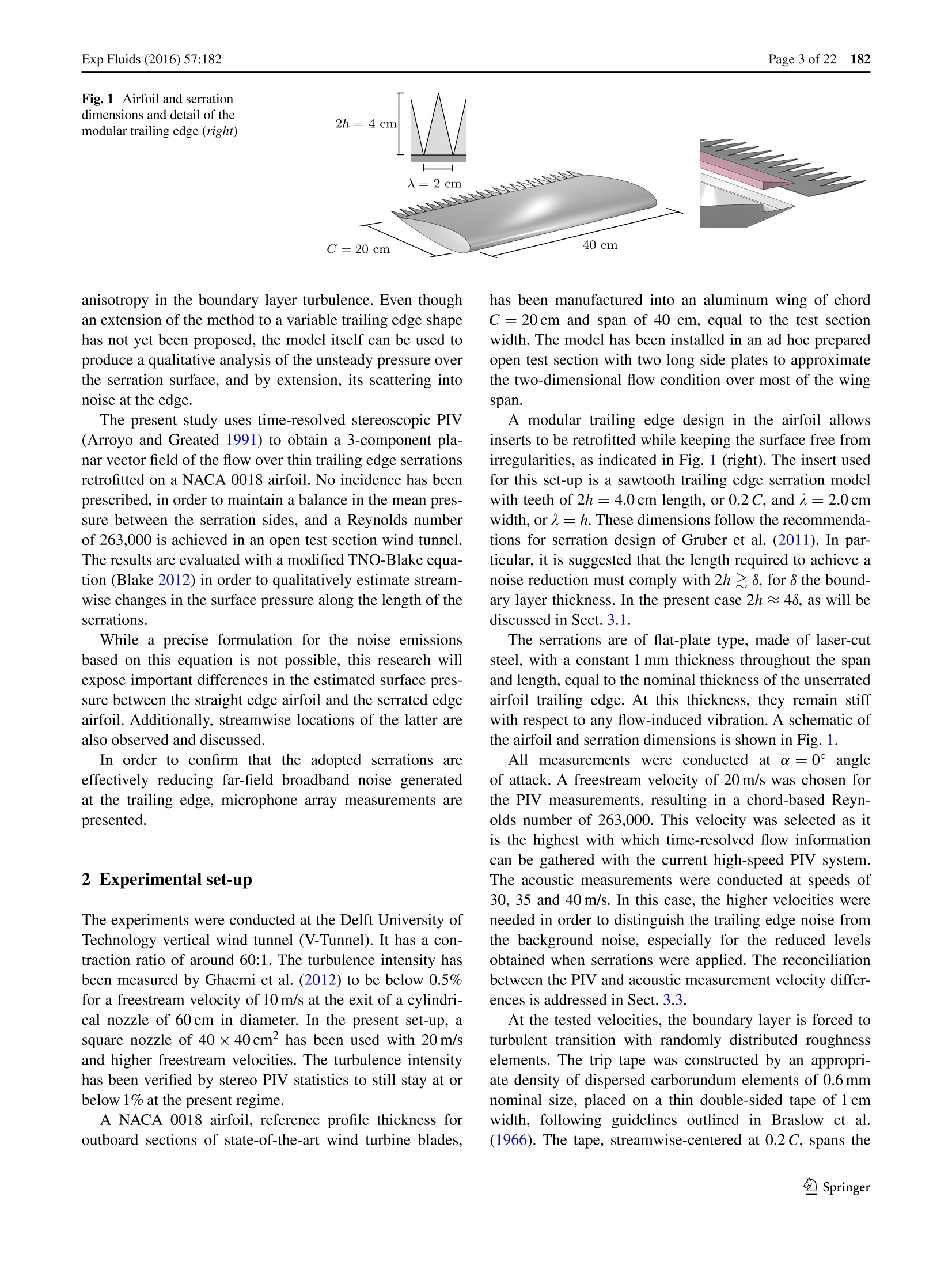
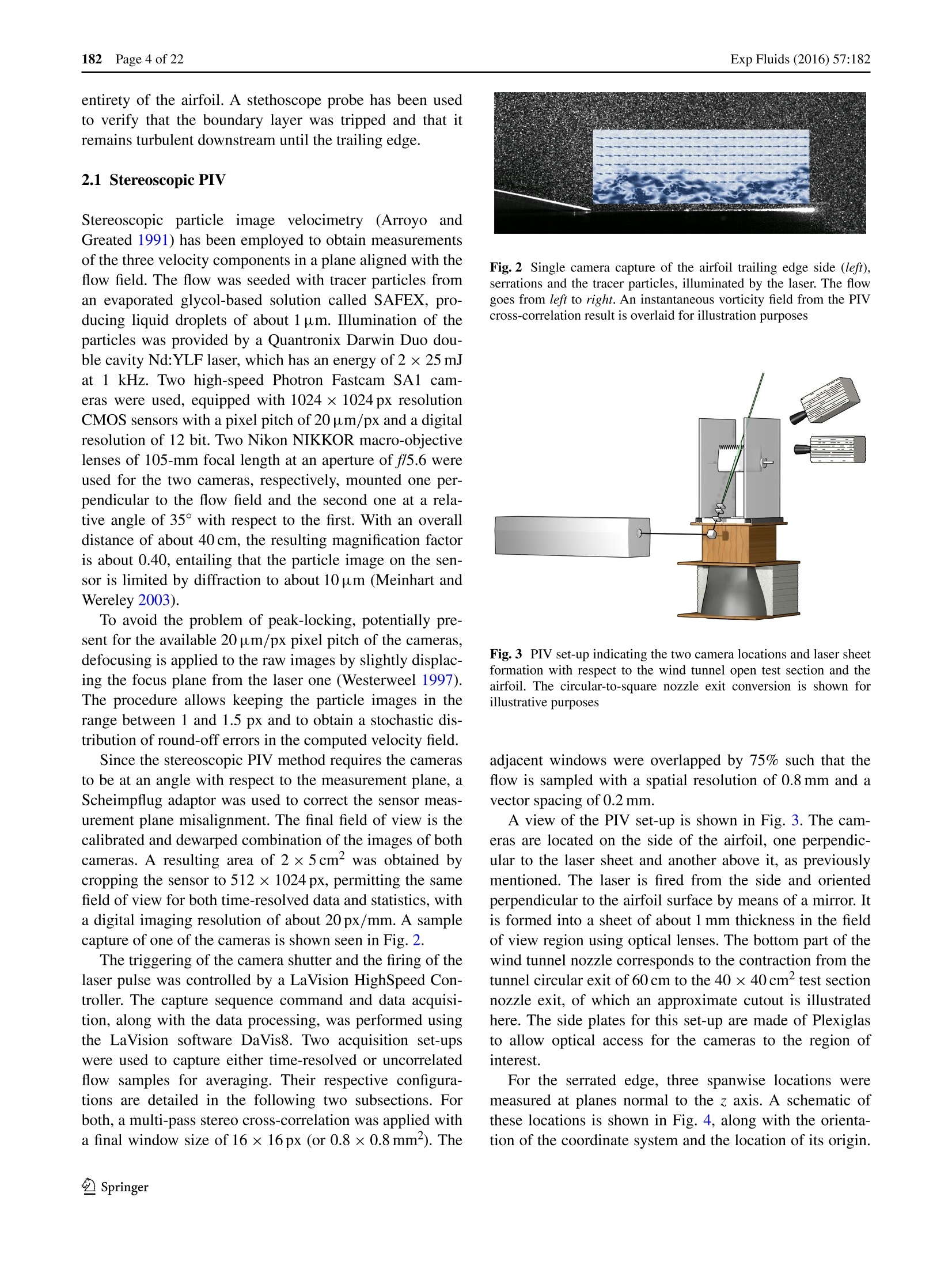
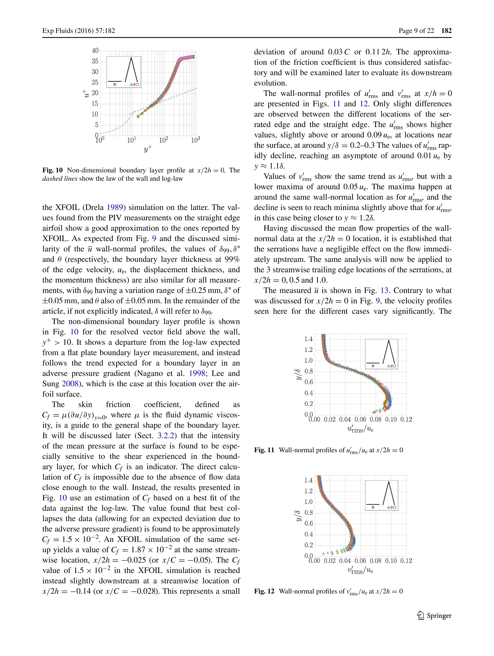
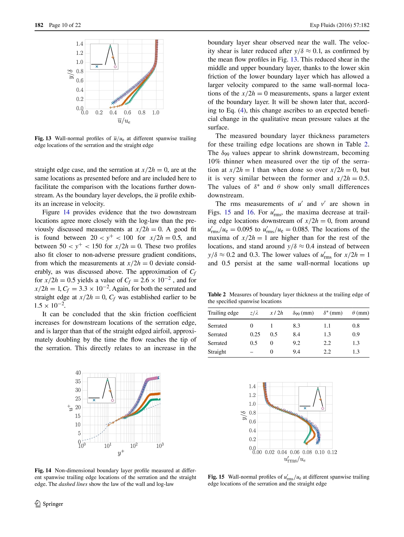
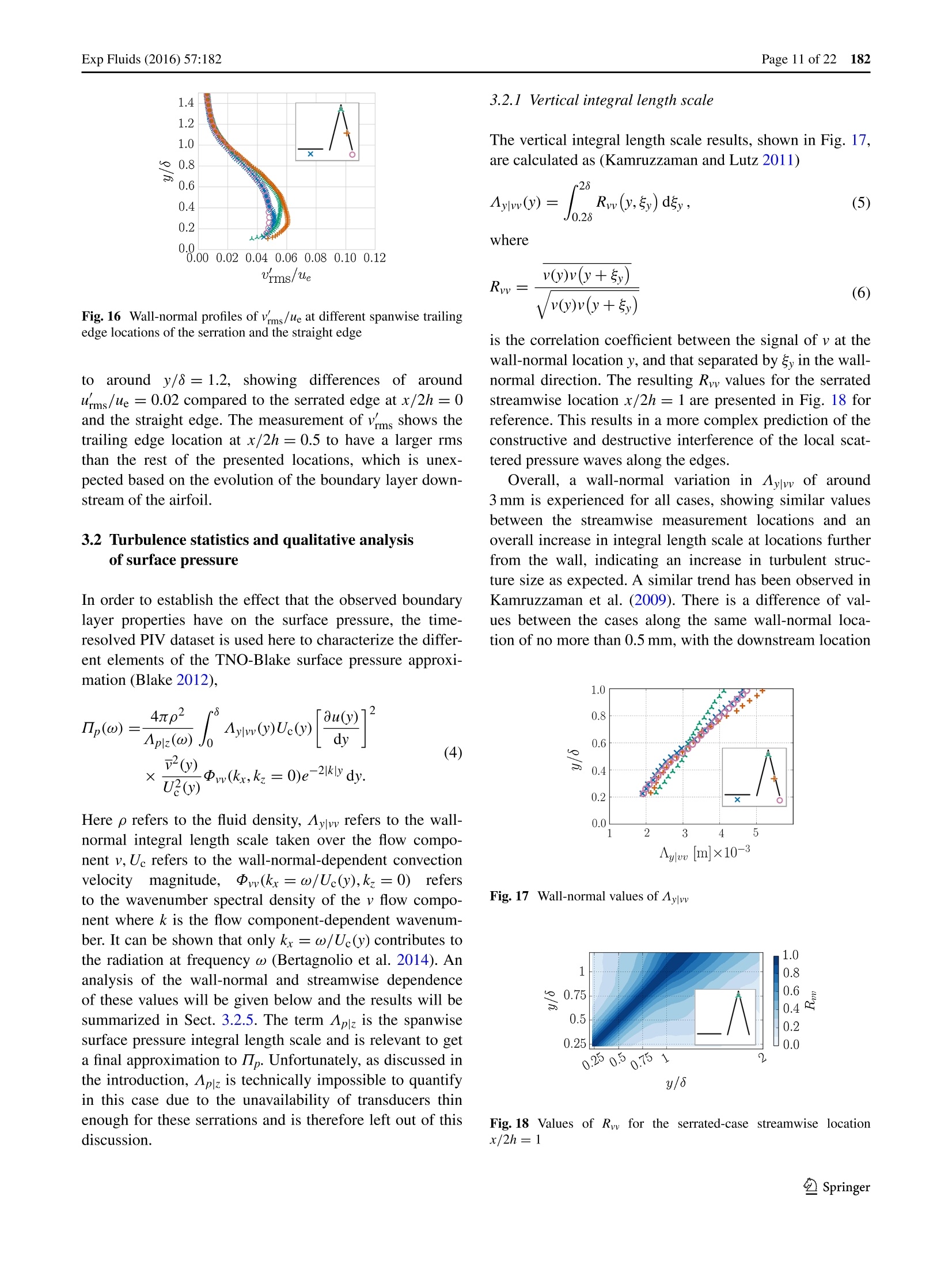
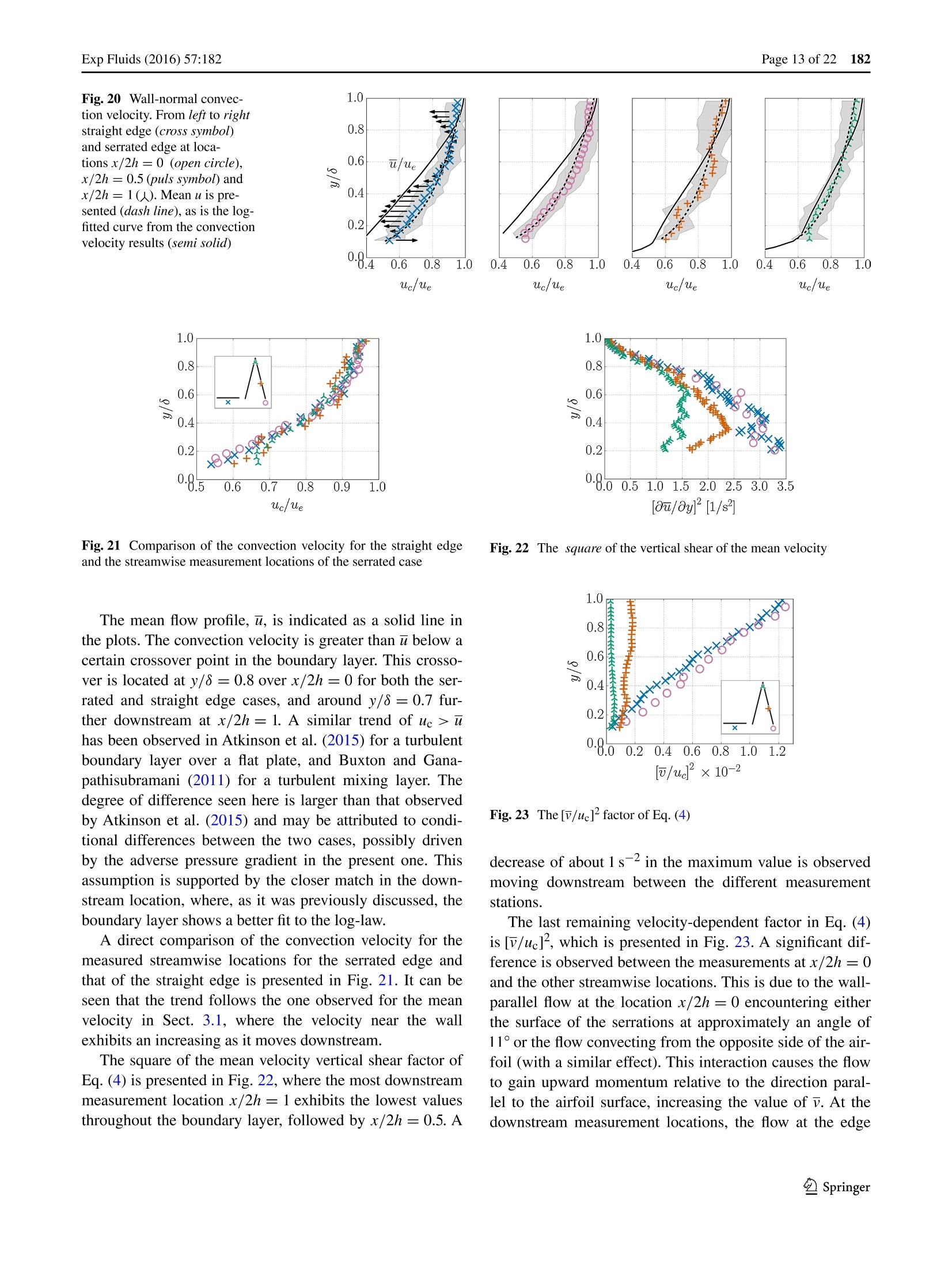
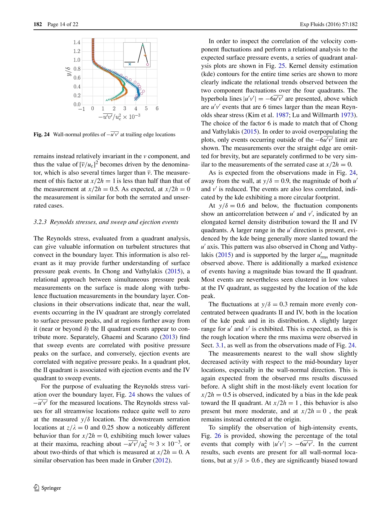
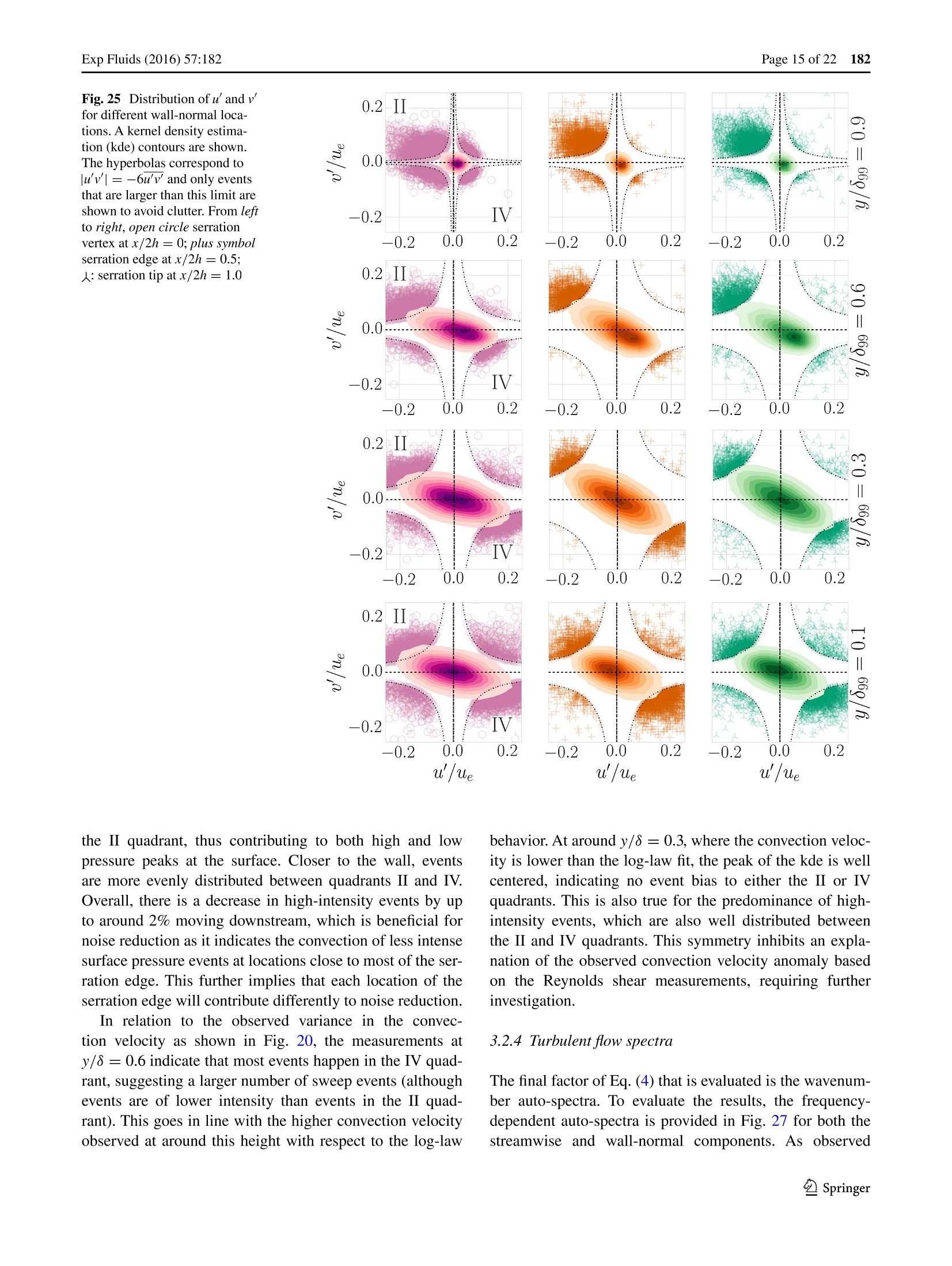
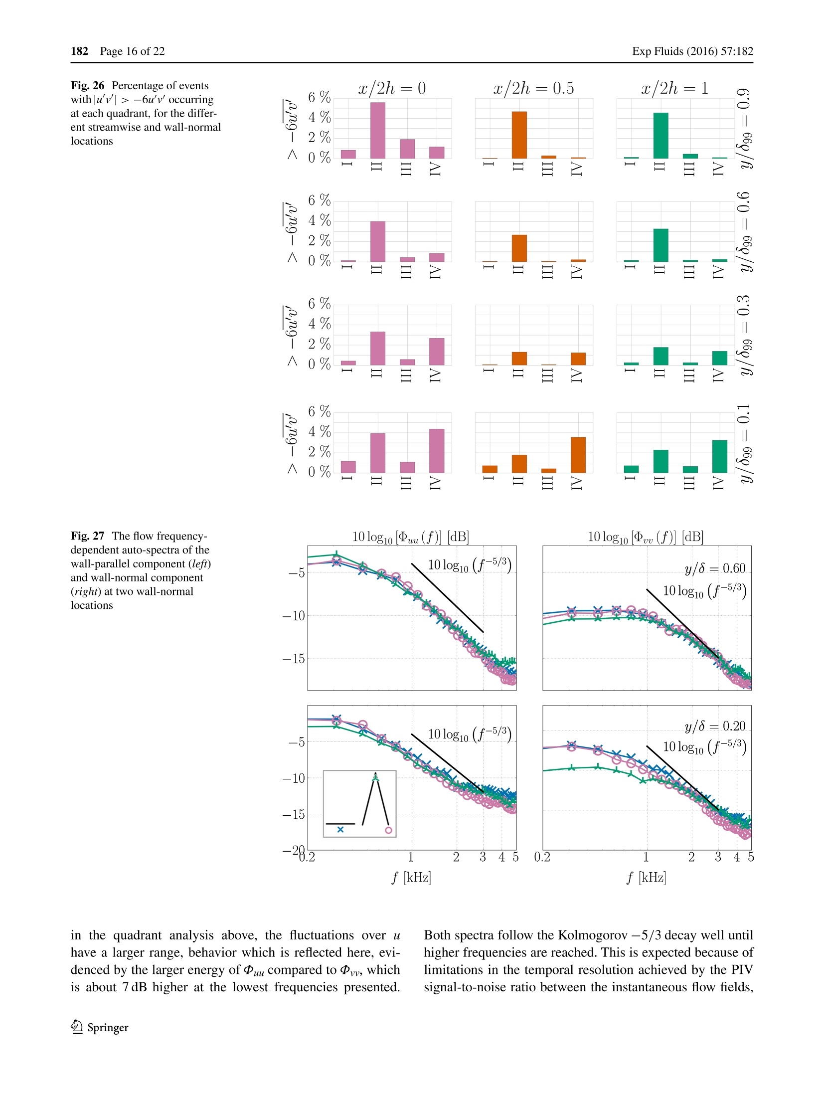
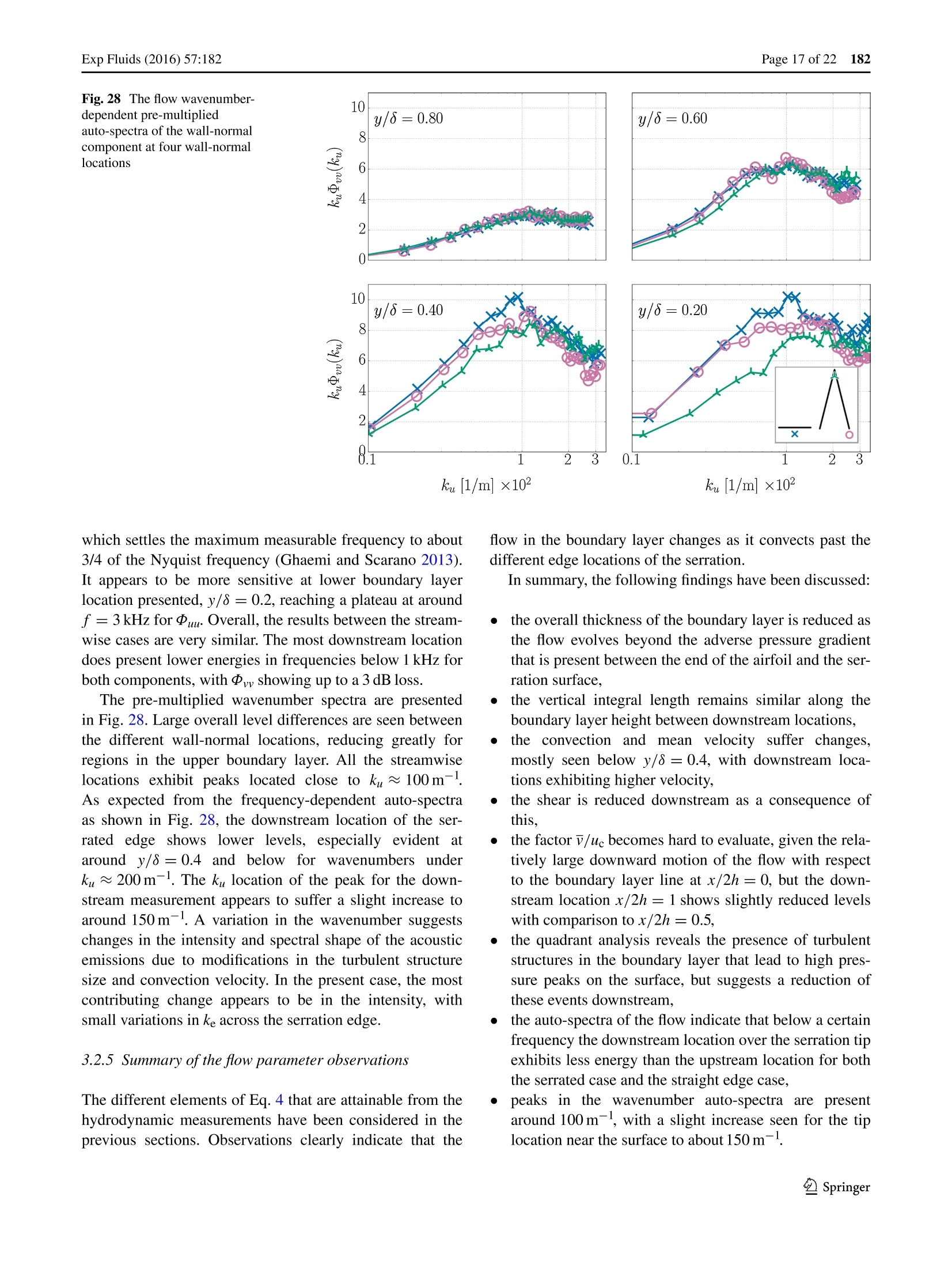
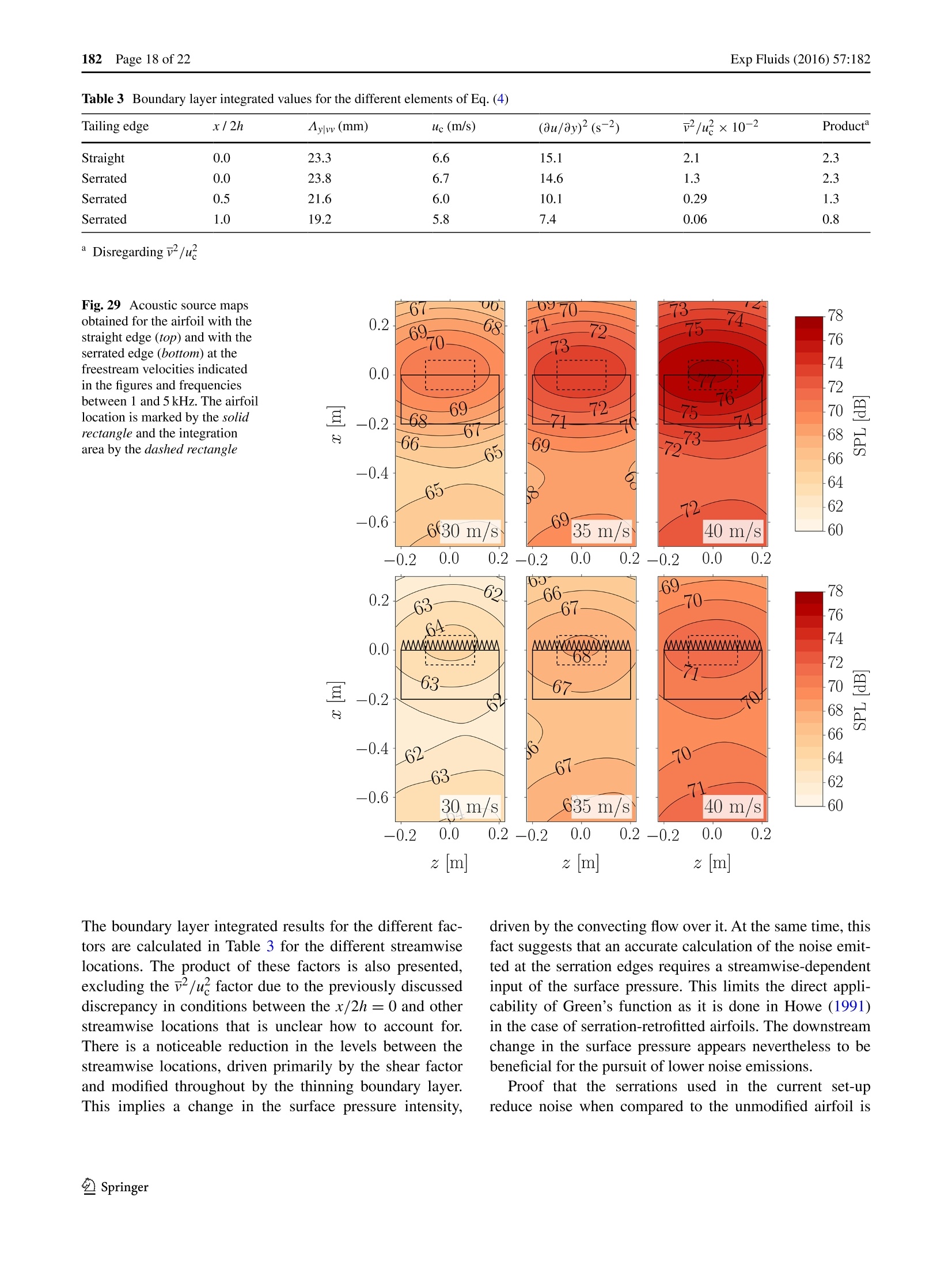
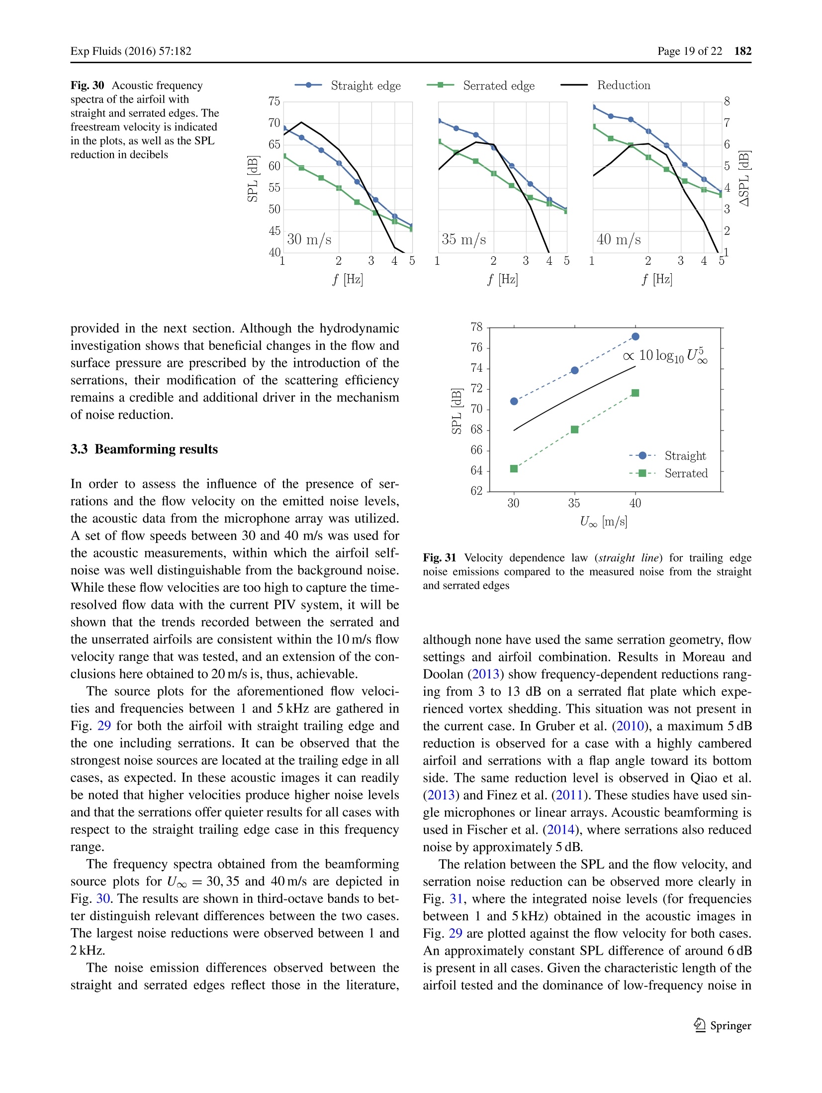
还剩21页未读,是否继续阅读?

产品配置单


北京欧兰科技发展有限公司为您提供《机翼翼型模型中流动的边界层特性和声学检测方案(粒子图像测速)》,该方案主要用于航空中流动的边界层特性和声学检测,参考标准--,《机翼翼型模型中流动的边界层特性和声学检测方案(粒子图像测速)》用到的仪器有德国LaVision PIV/PLIF粒子成像测速场仪、LaVision HighSpeedStar 高帧频相机、LaVision DaVis 智能成像软件平台
推荐专场


相关方案
更多
该厂商其他方案
更多