空气，液体流动中3D3C速度矢量场检测方案(粒子图像测速)

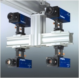
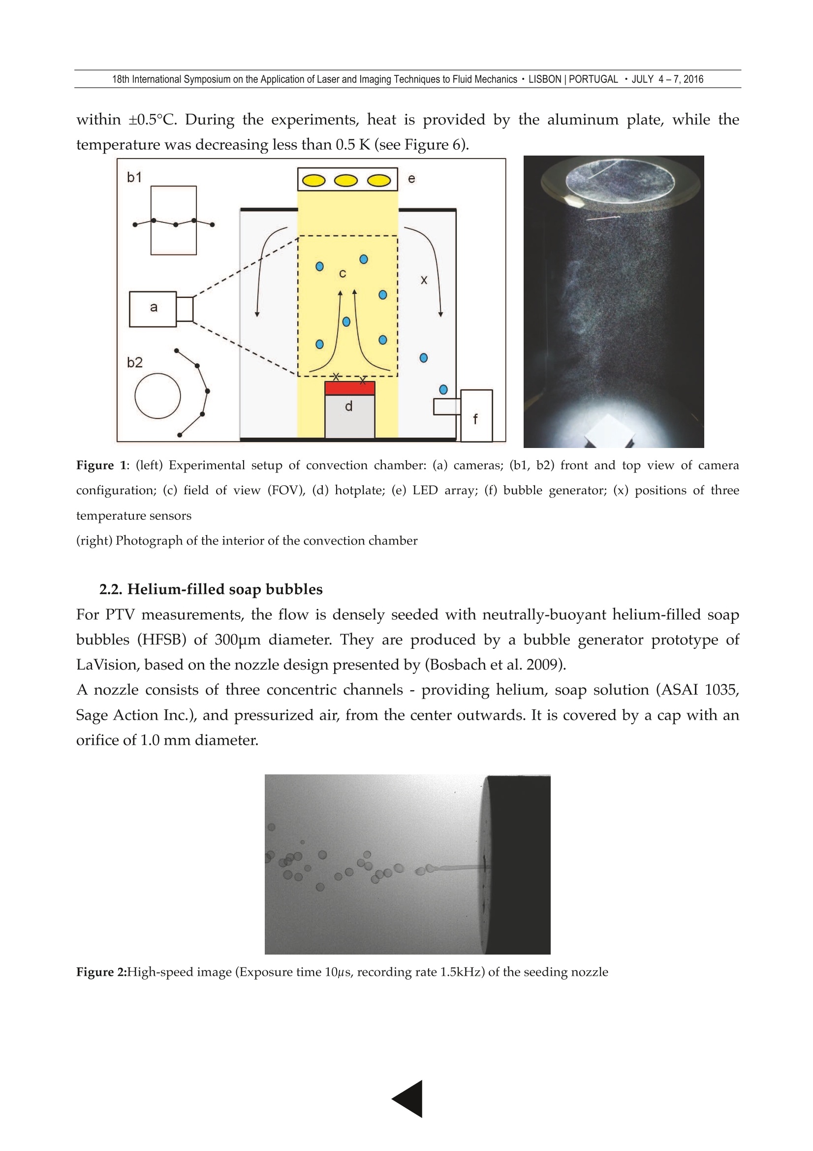
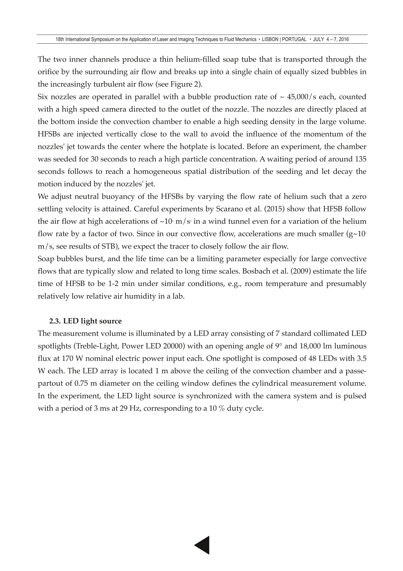
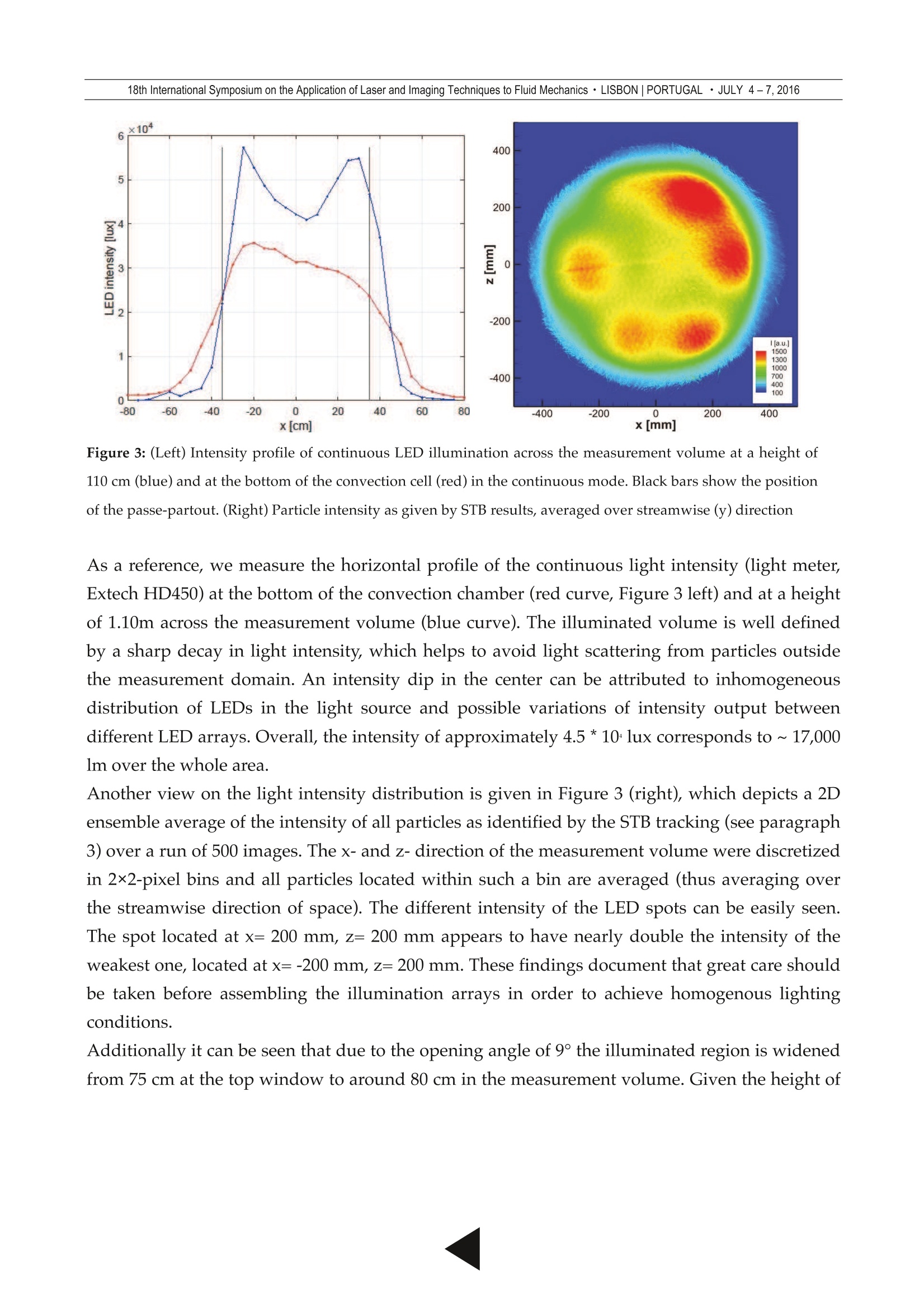
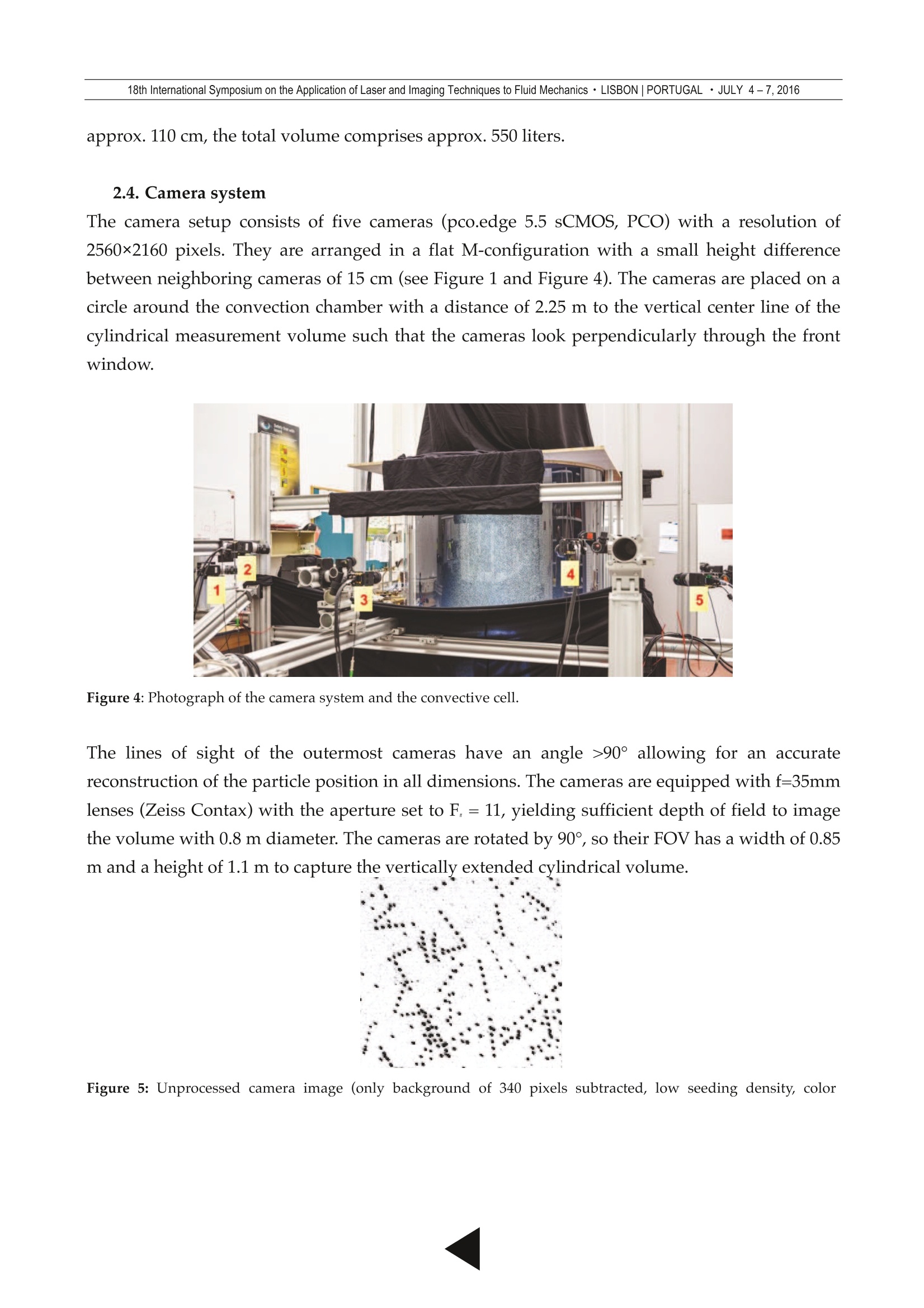
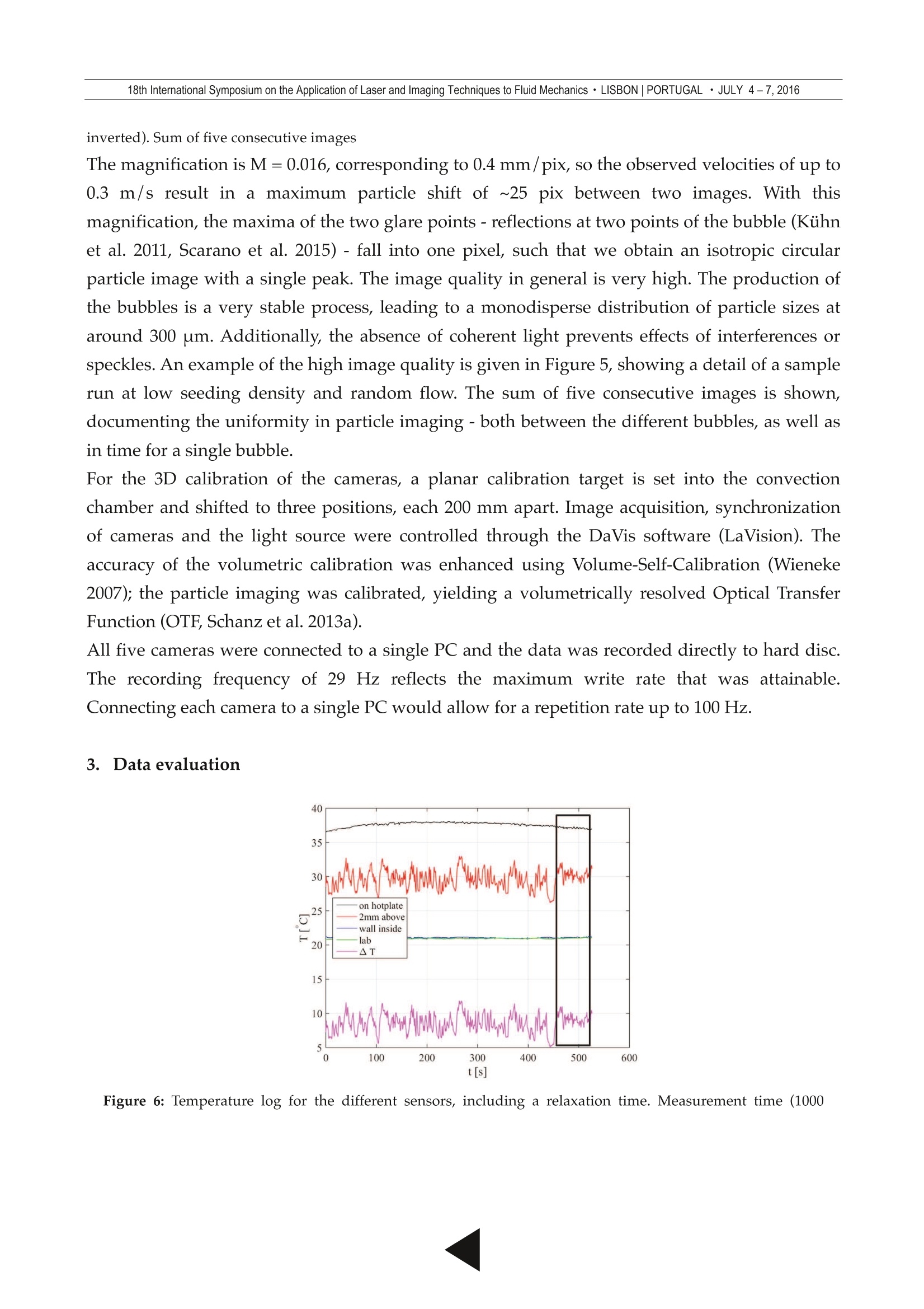
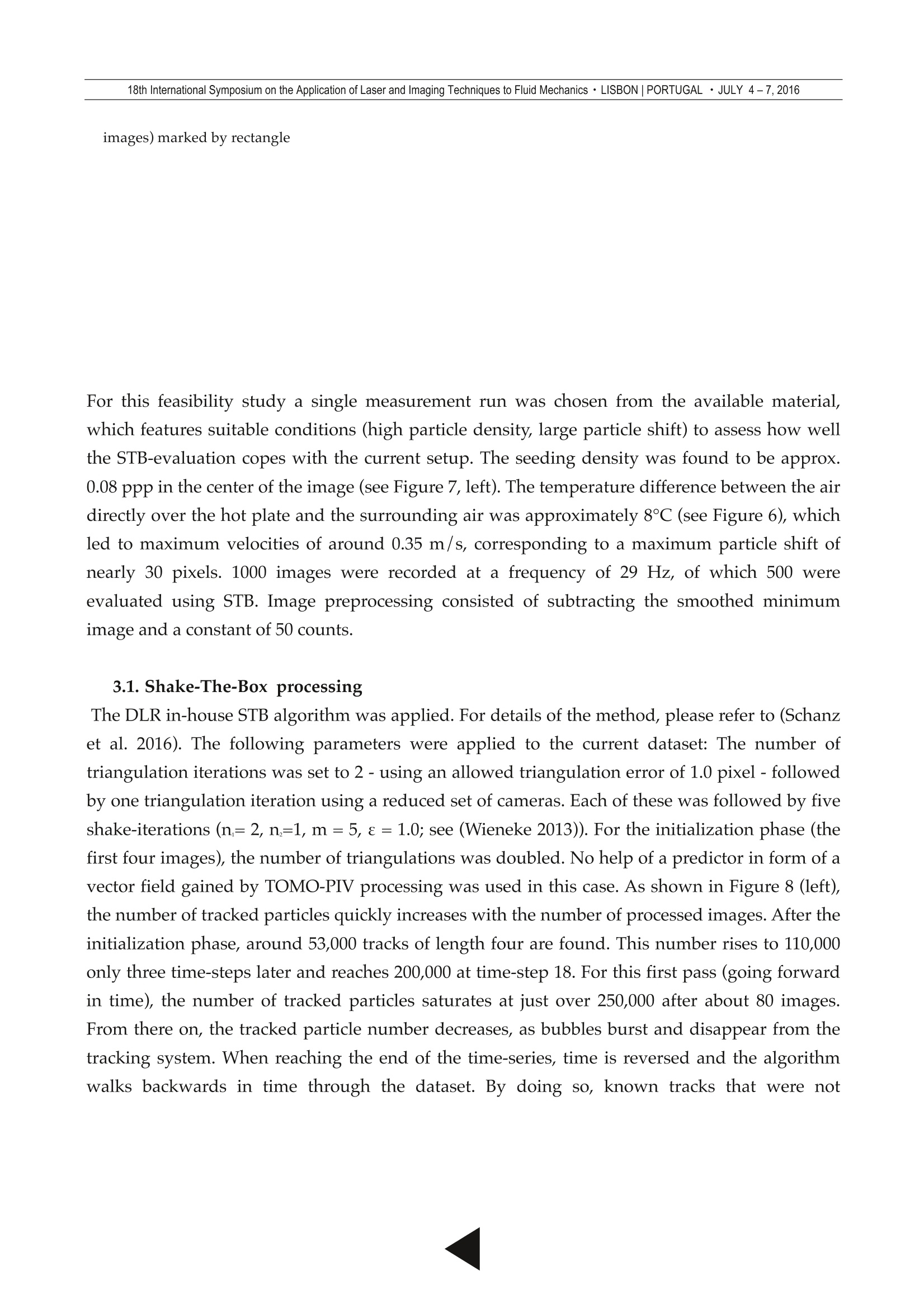
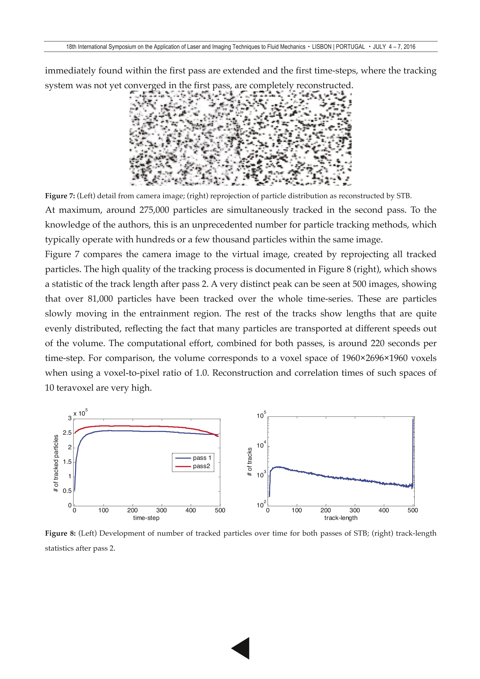
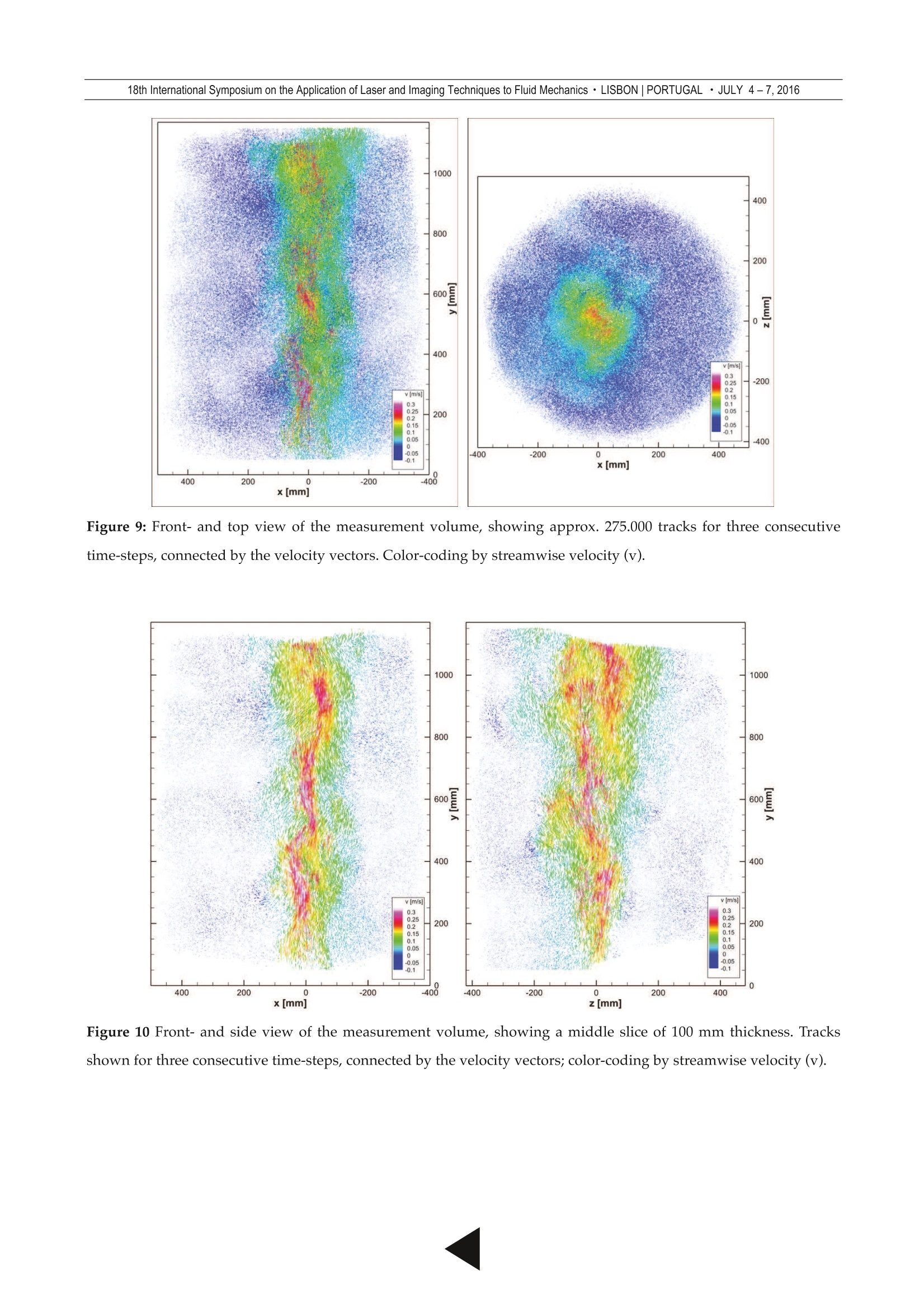
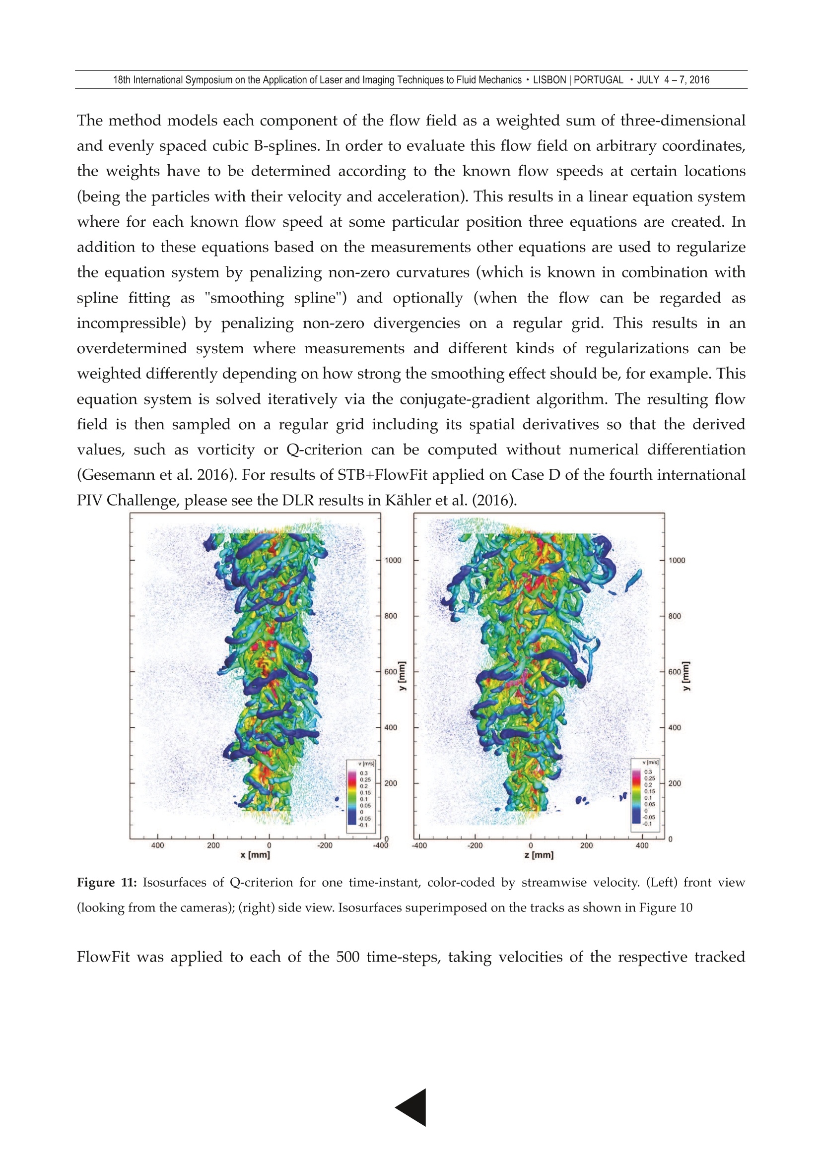
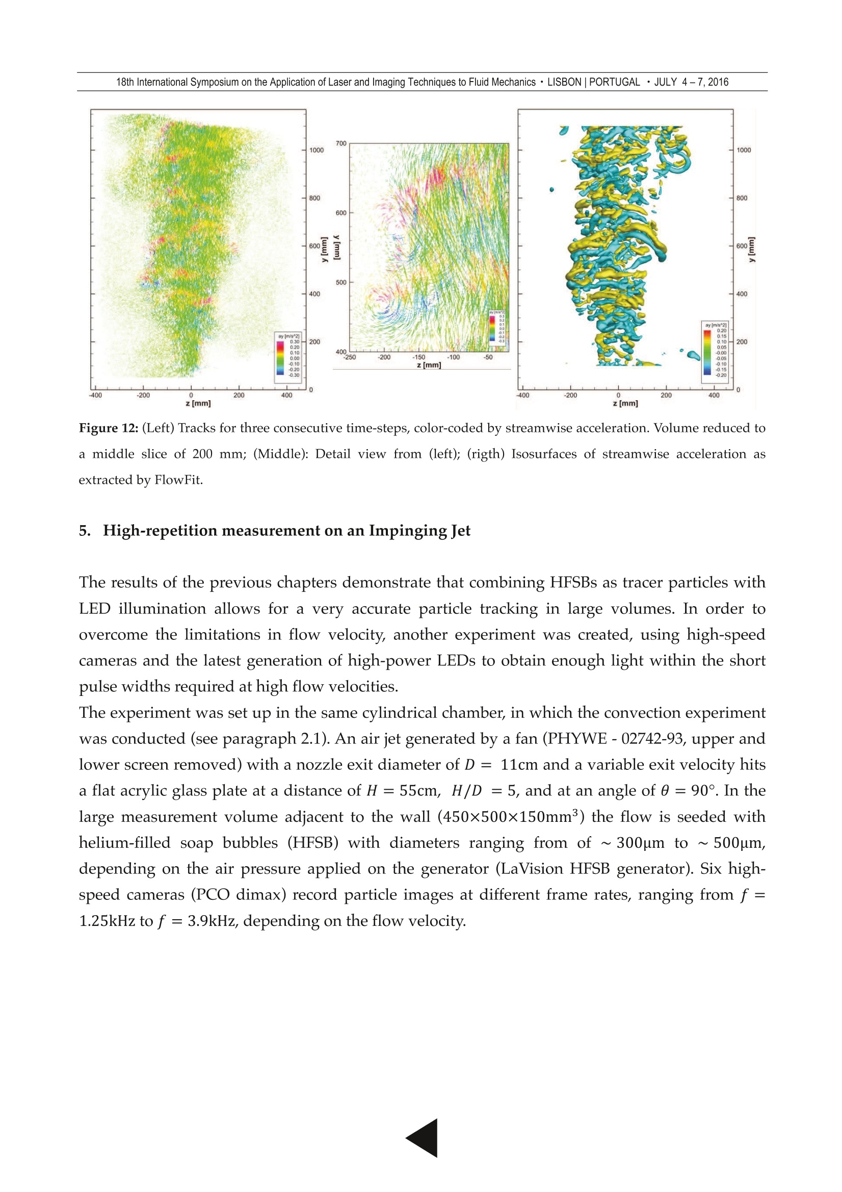
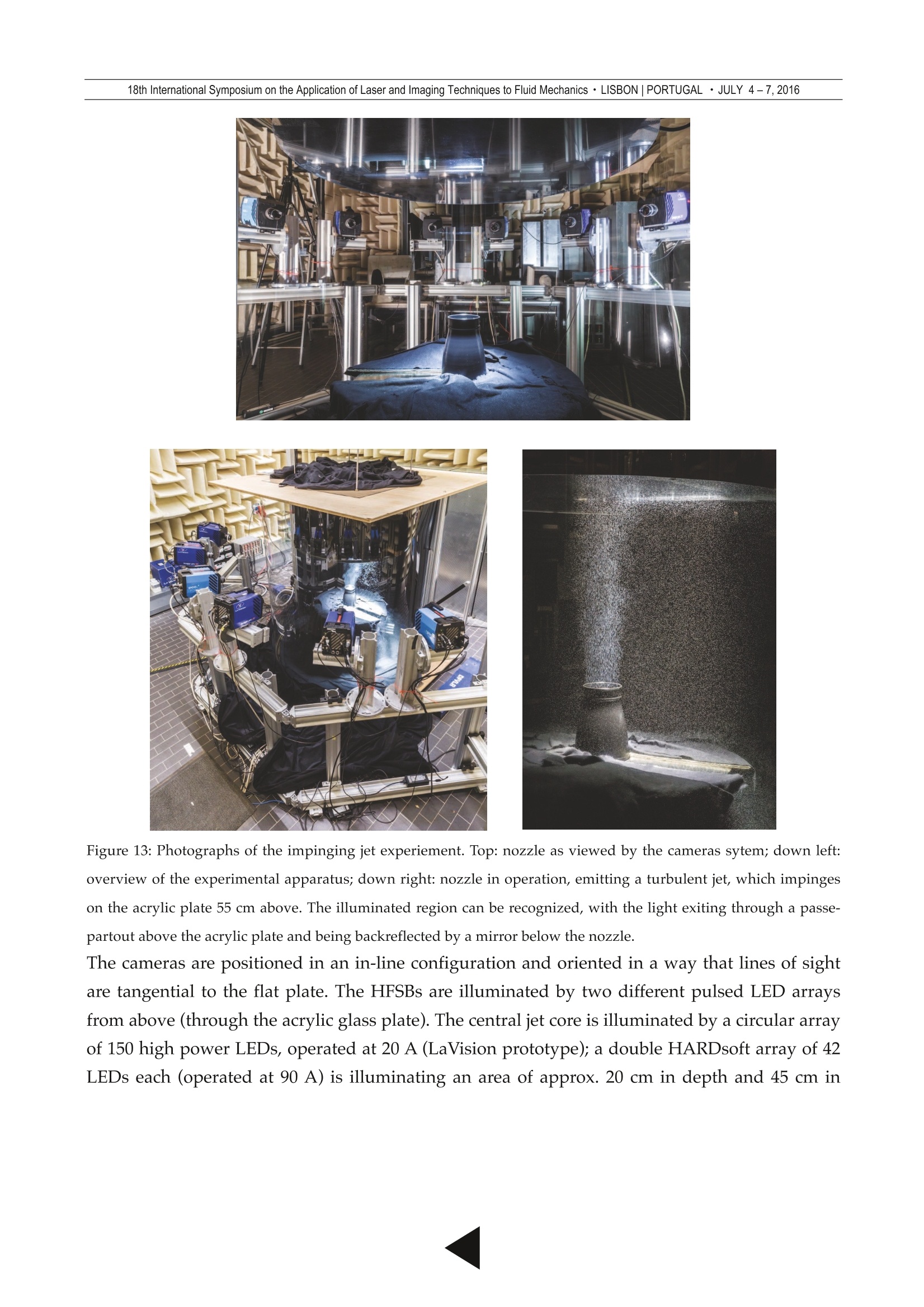
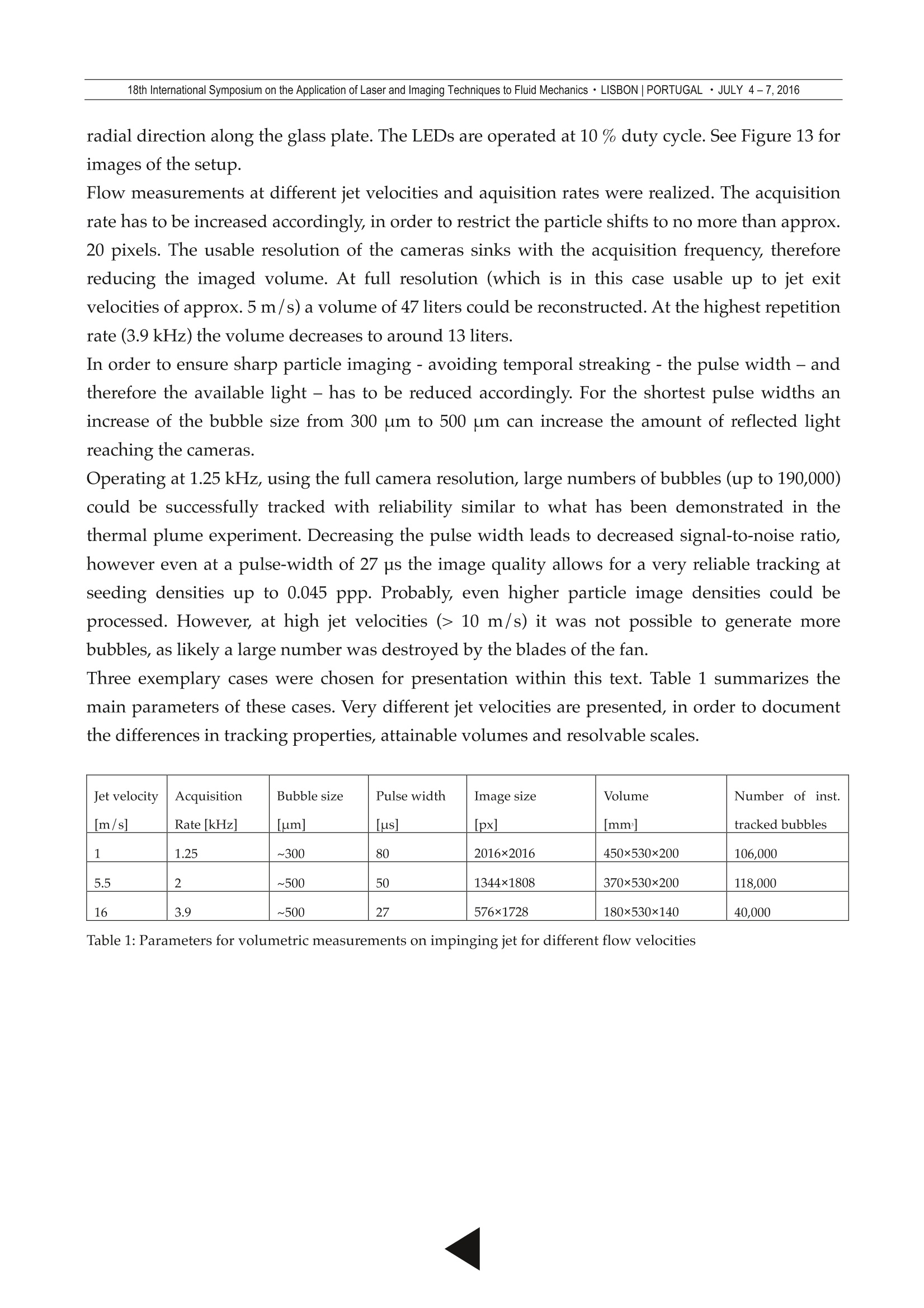
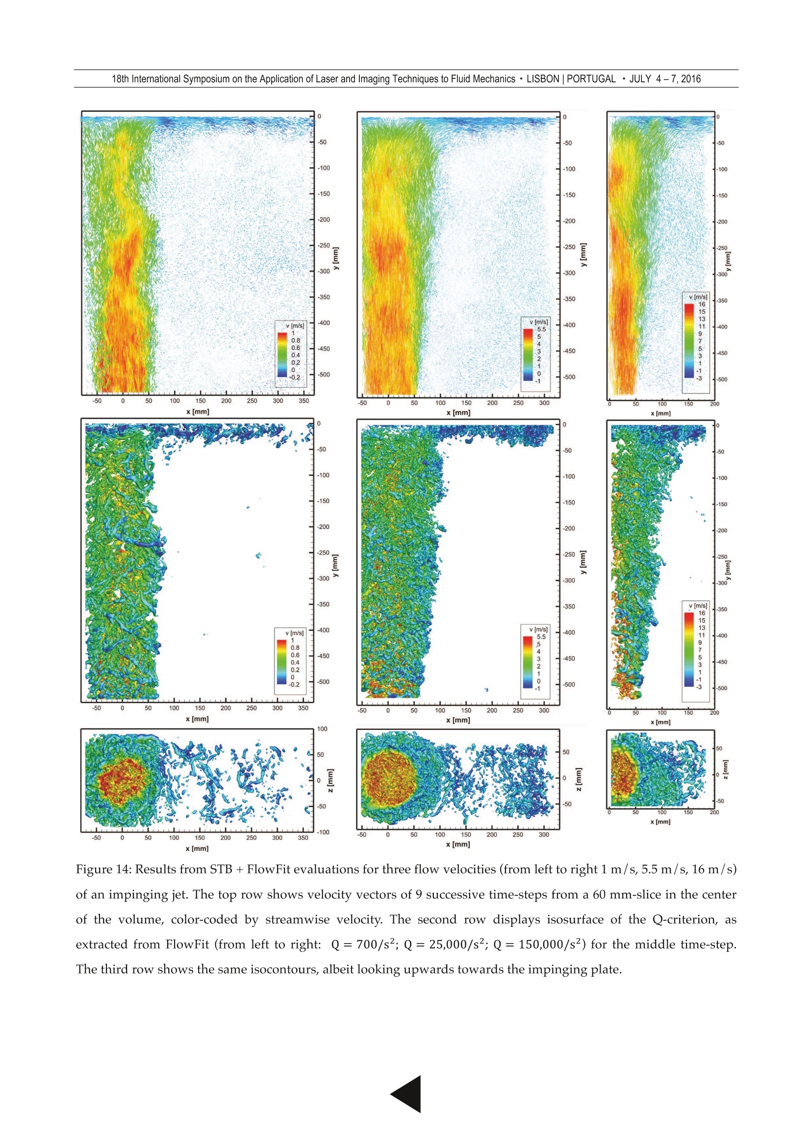
18th International Symposium on the Application of Laser and Imaging Techniques to Fluid Mechanics·LISBON|PORTUGAL ·JULY 4-7，2016 TUDelft Delft University of Technology Towards high-resolution 3D flow field measurements at cubic meter scales Schanz， Daniel； Huhn， Florian； Gesemann， Sebastian；Dierksheide，Uwe； van de Meerendonk， Remco；Manovski， P.； Schroder， Andreas Publication date2016 Document VersionFinal published version Published in Proceedings of the 18th International Symposium on the Application of Laser and Imaging Techniques toFluid Mechanics Citation (APA) Schanz， D.， Huhn， F.， Gesemann， S.，Dierksheide， U.， van de Meerendonk， R.， Manovski， P.， &Schroder，A. (2016). Towards high-resolution 3D flow field measurements at cubic meter scales. In Proceedings of the18th International Symposium on the Application of Laser and Imaging Techniques to Fluid Mechanics.Lisbon， Portugal： Springer Verlag. Important note To cite this publication， please use the final published version (if applicable). Please check the document version above. Copyright Other than for strictly personal use， it is not permitted to download， forward or distribute the text or part of it， without the consentof the author(s) and/or copyright holder(s)， unless the work is under an open content license such as Creative Commons. Takedown policy Please contact us and provide details if you believe this document breaches copyrights. We will remove access to the work immediately and investigate your claim. This work is downloaded from Delft University of Technology. For technical reasons the number of authors shown on this cover page is limited to a maximum of 10. PROCEEDINGS OF THE18thINTERNATIONALSYMPOSIUM ON APPLICATION OF LASER AND IMAGING TECHNIQUESTOFLUID MECHANICS Towards high-resolution 3D flow field measurements at cubic meter scales Daniel Schanz1， Florian Huhn1， Sebastian Gesemann1， Uwe Dierksheide?，Remco van de Meerendonk3， Peter Manovski4，Andreas Schroder1 1German Aerospace Center (DLR)， Institute of Aerodynamics and Flow Technology， Department of Experimental Methods， Gottingen， Germany； [daniel.schanz@dlr.de] 2LaVision GmbH， Anna-Vandenhoeck-Ring 19， Gottingen， Germany 3Aerospace Engineering Department， Delft University of Technology， 2629， The Netherlands 4Defence Science and Technology Organisation (DSTG)， Australia * Correspondent author： daniel.schanz@dlr.de Keywords： Lagrangian Particle Tracking， LED volume illumination， Helium filled soap bubbles ABSTRACT We present results from two large-volume volumetric flow experiments. The first of these， investigating a thermalplume at low velocities (up to 0.35 m/s) demonstrates the abilities and requirements to reach volume sizes up toand probably beyond one cubic meter. It is shown that the use of Helium filled soap bubbles (HFSBs) as tracers，combined with pulsed LED illumination yields high particle image quality over large volume depths. A veryuniform particle imaging， both in space as well as in time enables using high particle image concentrations (up to 0.1ppp)， while still being able to accurately reconstruct the flow using Shake-The-Box particle tracking. The experiment consisted of time-resolved volumetric flow measurements of a convectional plume within a volumeof approx. 0.55 m(550 liters). The light yield needed for such a large scale measurement is realized by using HFSBswith 300 um diameter as tracers and illuminating the measurement region using high-power， scalable arrays ofwhite LEDs. Applying the Shake-The-Box algorithm， up to 275，000 bubbles could be tracked simultaneously.Interpolating the results on a regular grid (using FlowFit') reveals a multitude of flow structures. The setup canbescaled to larger volumes of several cubic meters， basically only being limited by the number and power of availableLEDs and high-resolution cameras with sufficient frame-rate and pixel sizes. A second experiment showcases the possibilities to reach higher flow velocities， while still measuring within acomparatively large volume， by applying high-speed imaging and advanced LED illumination. An impingingturbulent jet was investigated in volumes ranging from 13 to 47 liters， depending on the repetition rate of the camerasystem. The results show that even at a repetition rate of 3.9 kHz and flow speeds up to 17 m/s the tested systemwas able to deliver images that allowed for a reliable and accurate tracking of bubbles. Again， the use of more LEDs would allow for larger volumes. New generations of high-speed cameras shouldenable the use of even higher flow speeds -thus enabling large-volume measurements in typical low speed windtunnel experiments at high spatial resolution (provided enough HFSBs can be produced). 1. Introduction and Motivation Time resolved volumetric flow measurements， using methods like TOMO PIV (Elsinga et al.2006)， 3D PTV (Maas et al. 1993， Malik et al. 1993) or Shake-The-Box (Schanz et al. 2016)， aretypically restricted to relatively small volume sizes in the order of <= 200 cm (Scarano et al.2015). This limitation stems from the small size of commonly used seeding material， in order toaccurately follow the flow (~ 1 um in air， 10 - 50 um in water). Currently available high-repetition laser systems， which are typically used as light source， do not provide enoughintensity to allow for illumination of larger volumes - even for the larger particles used in waterexperiments. However， seeding particles whose density approaches that of the medium can be ofmuch larger size， while still accurately following the flow (Melling 1997). Following this thought，neutrally buoyant Helium filled soap bubbles (HFSB) have been used in air to allow for largescale flow measurements. Applications range from traceline-visualizations (Pounder 1956) overlarge-scale 2D-PIV measurements (Miiller et al. 2000， Bosbach et al. 2009) to three-dimensionaltracking of single bubbles (Klimas 1973) and large-scale tomographic PIV of a convective flow(Kuhn et al. 2011). Very recently， the feasibility of using HFSBs in wind tunnel facilities has beendemonstrated (Scarano 2015). While some the previous applications examined large measurement areas (Biwole et al. 2009，Klimas 1973)， all of these were limited in particle number (e. g. tracing a few tens or hundreds ofbubbles). The largest investigated volume that allowed the description of instantaneous flowstructures was applied by Kihn et al (2011). A convection cell with a volume of approx. 56 literswas investigated using 2-pulse tomo-PIV. However， a large interrogation window size had to bechosen (48*48*24 mm)， limiting the spatial resolution to large structures. The experimentreported by Scarano et al. (2015) was special in that it is the first application of HFBSs in a windtunnel experiment. As Scarano et al. have shown， the production of enough bubbles to achieve asufficient particle concentration within the measurement volume is a major topic for higher flowspeeds. Due to the limitations in bubble number and due to the limits of the high-speed laserused for illumination， the volume size was restricted to 4.8 liters in this experiment and theinterrogation windows were quite large (96x96x86 voxels). The experiments discussed here avoid the problem of bubble production rate by operating in aclosed chamber. LEDs provide a scalable light-source that is free of the typical artifacts of laserillumination (speckles， diffraction problems， etc.). HFSBs can be produced virtually mono-disperse and due to the light being reflected at the bubble surface (instead of scattered) unevenimaging between the different cameras is avoided. These features lead to a very high attainableimage quality (as discussed in paragraph 2.4)， which allows for a very reliable and accurateparticle tracking using the Shake-The-Box((STB) algorithm. By applyinga regularizedinterpolation scheme (FlowFit'， Gesemann et al. 2016) the locally highly accurate information isleveraged to maximize the spatial resolution (Schneiders et al. 2015). 2.. Thermal plume investigation 2.1. Convection chamber The experiments are performed in a cylindrical convection chamber with a height of 2.00 m anda diameter of 1.83 ，m (see Figure 1). Top and bottom plates are constructed of wood， the backwall is made of aluminum， and the transparent front window is acrylic glass of 1 mm thickness.Intransparent parts of the floor， walls and ceiling are painted black or covered with blackadhesive film， in order to avoid scattered light and to improve the contrast of the particle imagestowards the background. The convection chamber is accessible from the back side through adoor in the aluminum wall. The chamber is equipped with a circular perforated tube at thebottom to rinse it with pressurized air and remove seeding. LED illumination enters through a plexiglas window of 1 m diameter in the ceiling， covered witha circular passe-partout (0.75 m diameter) that determines the width of the cylindricalmeasurement volume. The convective flow is forced by a standard 1500 W electric hotplate (188mm diameter， Silva Homeline EKS 2121) that is placed a few centimeters below the measurementvolume. It is covered by a black circular 250 mm diameter aluminum plate of 10 mm thicknessthat serves as a heat reservoir to keep the temperature constant over time. Before conducting experiments， the hotplate is heated up for a few seconds to reach the desiredtemperature， and left some minutes until a uniform temperature distribution and a constanttemperature is attained. Three temperature sensors are installed in the convection chamber tomonitor the temperature of the heated aluminum plate， the air temperature 2 mm above theplate as a proxy for the maximum air temperature， and the ambient air temperature (see Figure 1for positions of sensors). The accuracy of the absolute temperature measurement is estimated tobe ±2C， while the relative temperature differences， relevant for the convective flow， are accurate within ±0.5℃. During the experiments， heat is provided by the aluminum plate， while thetemperature was decreasing less than 0.5 K (see Figure 6). Figure 1： (left) Experimental setup of convection chamber： (a) cameras； (b1， b2) front and top view of cameraconfiguration； (c) field of view (FOV)， (d) hotplate； (e) LED array； (f) bubble generator；(x) positions of threetemperature sensors (right) Photograph of the interior of the convection chamber 2.2. Helium-filled soap bubbles For PTV measurements， the flow is densely seeded with neutrally-buoyant helium-filled soapbubbles (HFSB) of 300um diameter. They are produced by a bubble generator prototype ofLaVision， based on the nozzle design presented by (Bosbach et al. 2009). A nozzle consists of three concentric channels - providing helium， soap solution (ASAI 1035，Sage Action Inc.)， and pressurized air， from the center outwards. It is covered by a cap with anorifice of 1.0 mm diameter. Figure 2：High-speed image (Exposure time 10us， recording rate 1.5kHz) of the seeding nozzle The two inner channels produce a thin helium-filled soap tube that is transported through theorifice by the surrounding air flow and breaks up into a single chain of equally sized bubbles inthe increasingly turbulent air flow (see Figure 2). Six nozzles are operated in parallel with a bubble production rate of ~ 45，000/s each， countedwith a high speed camera directed to the outlet of the nozzle. The nozzles are directly placed atthe bottom inside the convection chamber to enable a high seeding density in the large volume.HFSBs are injected vertically close to the wall to avoid the influence of the momentum of thenozzles' jet towards the center where the hotplate is located. Before an experiment， the chamberwas seeded for 30 seconds to reach a high particle concentration. A waiting period of around 135seconds follows to reach a homogeneous spatial distribution of the seeding and let decay themotion induced by the nozzles'jet. We adjust neutral buoyancy of the HFSBs by varying the flow rate of helium such that a zerosettling velocity is attained. Careful experiments by Scarano et al. (2015) show that HFSB followthe air flow at high accelerations of ~10 m/s in a wind tunnel even for a variation of the heliumflow rate by a factor of two. Since in our convective flow， accelerations are much smaller (g~10m/s， see results of STB)， we expect the tracer to closely follow the air flow. Soap bubbles burst， and the life time can be a limiting parameter especially for large convectiveflows that are typically slow and related to long time scales. Bosbach et al. (2009) estimate the lifetime of HFSB to be 1-2 min under similar conditions， e.g.， room temperature and presumablyrelatively low relative air humidity in a lab. 2.3. LED light source The measurement volume is illuminated by a LED array consisting of 7 standard collimated LEDspotlights (Treble-Light， Power LED 20000) with an opening angle of 9° and 18，000 lm luminousflux at 170 W nominal electric power input each. One spotlight is composed of 48 LEDs with 3.5W each. The LED array is located 1 m above the ceiling of the convection chamber and a passe-partout of 0.75 m diameter on the ceiling window defines the cylindrical measurement volume.In the experiment， the LED light source is synchronized with the camera system and is pulsedwith a period of 3 ms at 29 Hz， corresponding to a 10 % duty cycle. Figure 3： (Left) Intensity profile of continuous LED illumination across the measurement volume at a height of110 cm (blue) and at the bottom of the convection cell (red) in the continuous mode. Black bars show the positionof the passe-partout. (Right) Particle intensity as given by STB results， averaged over streamwise (y) direction As a reference， we measure the horizontal profile of the continuous light intensity (light meter，Extech HD450) at the bottom of the convection chamber (red curve， Figure 3 left) and at a heightof 1.10m across the measurement volume (blue curve). The illuminated volume is well definedby a sharp decay in light intensity， which helps to avoid light scattering from particles outsidethe measurement domain. An intensity dip in the center can be attributed to inhomogeneousdistribution of LEDs in the light source and possible variations of intensity output betweendifferent LED arrays. Overall， the intensity of approximately 4.5 *10. lux corresponds to ~ 17，000lm over the whole area. Another view on the light intensity distribution is given in Figure 3 (right)， which depicts a 2Densemble average of the intensity of all particles as identified by the STB tracking (see paragraph3) over a run of 500 images. The x- and z- direction of the measurement volume were discretizedin 2x2-pixel bins and all particles located within such a bin are averaged (thus averaging overthe streamwise direction of space). The different intensity of the LED spots can be easily seen.The spot located at x= 200 mm， z= 200 mm appears to have nearly double the intensity of theweakest one， located at x=-200 mm， z= 200 mm. These findings document that great care shouldbe taken before assembling the illumination arrays in order to achieve homogenous lightingconditions. Additionally it can be seen that due to the opening angle of 9° the illuminated region is widenedfrom 75 cm at the top window to around 80 cm in the measurement volume. Given the height of approx. 110 cm， the total volume comprises approx. 550 liters. 2.4. Camera system The camera setup consists of five cameras (pco.edge 5.5 sCMOS， PCO) with a resolution of2560×2160 pixels. They are arranged in a flat M-configuration with a small height differencebetween neighboring cameras of 15 cm (see Figure 1 and Figure 4). The cameras are placed on acircle around the convection chamber with a distance of 2.25 m to the vertical center line of thecylindrical measurement volume such that the cameras look perpendicularly through the frontwindow. Figure 4： Photograph of the camera system and the convective cell. The lines of sight of the outermost cameras have an angle >90°allowing for an accuratereconstruction of the particle position in all dimensions. The cameras are equipped with f=35mmlenses (Zeiss Contax) with the aperture set to F.=11， yielding sufficient depth of field to imagethe volume with 0.8 m diameter. The cameras are rotated by 90°， so their FOV has a width of 0.85m and a height of 1.1 m to capture the vertically extended cylindrical volume. Figure 5： Unprocessed camera image (only background of 340 pixels subtracted， low seeding density， color inverted). Sum of five consecutive images The magnification is M = 0.016， corresponding to 0.4 mm/pix， so the observed velocities of up to0.3 m/s result in a maximum particle shift of ~25 pix between two images. With thismagnification， the maxima of the two glare points- reflections at two points of the bubble (Kiihnet al. 2011， Scarano et al. 2015)- fall into one pixel， such that we obtain an isotropic circularparticle image with a single peak. The image quality in general is very high. The production ofthe bubbles is a very stable process， leading to a monodisperse distribution of particle sizes ataround 300 um. Additionally， the absence of coherent light prevents effects of interferences orspeckles. An example of the high image quality is given in Figure 5， showing a detail of a samplerun at low seeding density and random flow. The sum of five consecutive images is shown，documenting the uniformity in particle imaging-both between the different bubbles， as well asin time for a single bubble. For the 3D calibration of the cameras， a planar calibration target is set into the convectionchamber and shifted to three positions， each 200 mm apart. Image acquisition， synchronizationof cameras and the light source were controlled through the DaVis software (LaVision). Theaccuracy of the volumetric calibration was enhanced using Volume-Self-Calibration (Wieneke2007)； the particle imaging was calibrated， yielding a volumetrically resolved Optical TransferFunction (OTF， Schanz et al. 2013a). All five cameras were connected to a single PC and the data was recorded directly to hard disc.The recording frequency of 29 Hz reflects the maximum write rate that was attainable.Connecting each camera to a single PC would allow for a repetition rate up to 100 Hz. 3. Data evaluation Figure 6： Temperature log for the different sensors， including a relaxation time. Measurement time (1000 images) marked by rectangle For this feasibility study a single measurement run was chosen from the available material，which features suitable conditions (high particle density， large particle shift) to assess how wellthe STB-evaluation copes with the current setup. The seeding density was found to be approx.0.08 ppp in the center of the image (see Figure 7， left). The temperature difference between the airdirectly over the hot plate and the surrounding air was approximately 8℃ (see Figure 6)， whichled to maximum velocities of around 0.35 m/s， corresponding to a maximum particle shift ofnearly 30 pixels. 1000 images were recorded at a frequency of 29 Hz， of which 500 wereevaluated using STB. Image preprocessing consisted of subtracting the smoothed minimumimage and a constant of 50 counts. 3.1. Shake-The-Box processing The DLR in-house STB algorithm was applied. For details of the method， please refer to (Schanzet al. 2016). The following parameters were applied to the current dataset： The number oftriangulation iterations was set to 2 - using an allowed triangulation error of 1.0 pixel - followedby one triangulation iteration using a reduced set of cameras. Each of these was followed by fiveshake-iterations (n.=2， n=1， m=5， e=1.0； see (Wieneke 2013)). For the initialization phase (thefirst four images)， the number of triangulations was doubled. No help of a predictor in form of avector field gained by TOMO-PIV processing was used in this case. As shown in Figure 8 (left)，the number of tracked particles quickly increases with the number of processed images. After theinitialization phase， around 53，000 tracks of length four are found. This number rises to 110，000only three time-steps later and reaches 200，000 at time-step 18. For this first pass (going forwardin time)， the number of tracked particles saturates at just over 250，000 after about 80 images.From there on， the tracked particle number decreases， as bubbles burst and disappear from thetracking system. When reaching the end of the time-series， time is reversed and the algorithmwalks backwards in time through the dataset. By doing so， known tracks that were not Figure 7： (Left) detail from camera image； (right) reprojection of particle distribution as reconstructed by STB. At maximum， around 275，000 particles are simultaneously tracked in the second pass. To theknowledge of the authors， this is an unprecedented number for particle tracking methods， whichtypically operate with hundreds or a few thousand particles within the same image. Figure 7 compares the camera image to the virtual image， created by reprojecting all trackedparticles. The high quality of the tracking process is documented in Figure 8 (right)， which showsa statistic of the track length after pass 2. A very distinct peak can be seen at 500 images， showingthat over 81，000 particles have been tracked over the whole time-series. These are particlesslowly moving in the entrainment region. The rest of the tracks show lengths that are quiteevenly distributed， reflecting the fact that many particles are transported at different speeds outof the volume. The computational effort， combined for both passes， is around 220 seconds pertime-step. For comparison， the volume corresponds to a voxel space of 1960×2696×1960 voxelswhen using a voxel-to-pixel ratio of 1.0. Reconstruction and correlation times of such spaces of10 teravoxelare very high. Figure 8： (Left) Development of number of tracked particles over time for both passes of STB； (right) track-lengthstatistics after pass 2. Following the second pass， the particle tracks are temporally filtered by means of an optimalWiener filter， being represented by a series of 1D-B-Splines. On average， the particles are moved0.116 px from their original position (0.046 px in x-， 0.040 px in y-and 0.083 px in z-direction) bythe fit procedure. The velocity- and acceleration values are calculated as derivatives of thepolynomial. 4. Flow field results Figure 9 shows an instantaneous flow situation， depicted by ca. 275，000 tracks， whose velocityvectors are drawn for three consecutive time-steps and color-coded by streamwise velocity.Views from the front side and the top are provided. A large region of slowly moving particles，surrounding the thermal plume can be seen. The maximum velocity values are approx. 0.35 m/s，corresponding to a particle shift of nearly 30 pixels. The central regions can be better recognizedin Figure 10， which shows the same tracks as Figure 9， albeit only a middle slice of 10 cm depth isshown， both for the x/y-and the z/ y-plane. In general， the shape of the plume was varying intime quite visibly； in this time instant it can be seen that the plume is broadened in the z-direction， compared to the x-direction. Vortical structures can already be identified by looking at the particle tracks； however aquantitative description is possible when quantities like vorticity or the Q-criterion are available.To this end， the discrete Lagrangian velocity- and acceleration information at the particle locationis interpolated onto an Eulerian grid using the DLR in-house algorithm ‘FlowFit’ (Gesemann etal.2016). Figure 9： Front- and top view of the measurement volume， showing approx. 275.000 tracks for three consecutivetime-steps， connected by the velocity vectors. Color-coding by streamwise velocity (v). 1000 . 800 600E> 400 v[m 200 -0.05 -0.1 -400 -200 0 200 400 z [mm] Figure 10 Front- and side view of the measurement volume， showing a middle slice of 100 mm thickness. Tracksshown for three consecutive time-steps， connected by the velocity vectors； color-coding by streamwise velocity (v). The method models each component of the flow field as a weighted sum of three-dimensionaland evenly spaced cubic B-splines. In order to evaluate this flow field on arbitrary coordinates，the weights have to be determined according to the known flow speeds at certain locations(being the particles with their velocity and acceleration). This results in a linear equation systemwhere for each known flow speed at some particular position three equations are created. Inaddition to these equations based on the measurements other equations are used to regularizethe equation system by penalizing non-zero curvatures (which is known in combination withspline fitting as "smoothing spline") and optionally (when the flow can be regarded asincompressible) by penalizing non-zero divergencies on a regular grid. This results in anoverdetermined system where measurements and different kinds of regularizations can beweighted differently depending on how strong the smoothing effect should be， for example. Thisequation system is solved iteratively via the conjugate-gradient algorithm. The resulting flowfield is then sampled on a regular grid including its spatial derivatives so that the derivedvalues， such as vorticity or Q-criterion can be computed without numerical differentiationGesemann et al. 2016). For results of STB+FlowFit applied on Case D of the fourth international PIV Challenge， please see the DLR results in Kahler et al. (2016). Figure 11： Isosurfaces of Q-criterion for one time-instant， color-coded by streamwise velocity. (Left) front view(looking from the cameras)； (right) side view. Isosurfaces superimposed on the tracks as shown in Figure 10 FlowFit was applied to each of the 500 time-steps， taking velocities of the respective tracked particles as data base. The B-spline system is setup， such that on average ten B-spline cells arepresent for every particle (0.1 particles per cell)， leading to a spacing of approx. 8 mm between thecells. The compressibility constraint was applied (which is reasonable in the first approximation，given the low velocities and temperature gradients present)， such that a penalization was put ondivergency. 1500 iterations of the conjugate-gradient algorithm are applied to solve the equationsystem. The resulting continuous function is closely sampled on a grid with 3 mm spacing，ultimately leading to vector volumes of 266x333×266 vectors. An example of the results gained by applying FlowFit to the STB track data is given in Figure 11，which shows isosurfaces of Q-criterion for the middle of the three time-steps shown in Figure 9and Figure 10. The full amount and extent of the thermal flow structures becomes apparent.Long， undisturbed vortices are identified in the shear layers surrounding the center of theplume， while the central structures are smaller， but show equal strength. When looking at a time-series of such images a high temporal coherence is noticeable. The high quality of the trackingprocess translates directly into the quality of the Eulerian representation. The high position accuracy， which is achievable due to the image quality， allows for anevaluation of particle acceleration (material derivative)-being the second derivative of space.Figure 12 shows tracks for the same time-steps as discussed before， color-coded by streamwiseacceleration. Especially the detail view reveals that the acceleration and deceleration of particlesdrawn into flow structures is rendered smoothly by the tracking scheme. Just as for velocity， theacceleration can be interpolated onto an Eulerian grid using FlowFit. Figure 12 (right) displaysthe result of applying FlowFit to the particle accleration distribution in Figure 12 (left)， with apenalization of rotation (therefore implying that viscosity effects plays a minor rule， whichshould hold for the small temperature differences present). Isosurfaces ofstream iseacceleration indicate the regions of acceleration and deceleration above and below vortices(compare to Figure 11， right). Figure 12： (Left) Tracks for three consecutive time-steps， color-coded by streamwise acceleration. Volume reduced toa middle slice of 200 mm； (Middle)： Detail view from (left)； (rigth) Isosurfaces of streamwise acceleration asextracted by FlowFit. 5. High-repetition measurement on an Impinging Jet The results of the previous chapters demonstrate that combining HFSBs as tracer particles withLED illumination allows for a very accurate particle tracking in large volumes. In order toovercome the limitations in flow velocity， another experiment was created， using high-speedcameras and the latest generation of high-power LEDs to obtain enough light within the shortpulse widths required at high flow velocities. The experiment was set up in the same cylindrical chamber， in which the convection experimentwas conducted (see paragraph 2.1). An air jet generated by a fan (PHYWE-02742-93， upper andlower screen removed) with a nozzle exit diameter of D = 11cm and a variable exit velocity hitsa flat acrylic glass plate at a distance of H=55cm， H/D =5， and at an angle of 0= 90°. In thelarge measurement volume adjacent to the wall (450×500×150mm) the flow is seeded withhelium-filled soap bubbles (HFSB) with diameters ranging from of ~ 300um to ~500um，depending on the air pressure applied on the generator (LaVision HFSB generator). Six high-speed cameras (PCO dimax) record particle images at different frame rates， ranging from f=1.25kHz to f = 3.9kHz， depending on the flow velocity. Figure 13： Photographs of the impinging jet experiement. Top： nozzle as viewed by the cameras sytem； down left：overview of the experimental apparatus； down right： nozzle in operation， emitting a turbulent jet， which impingeson the acrylic plate 55 cm above. The illuminated region can be recognized， with the light exiting through a passe-partout above the acrylic plate and being backreflected by a mirror below the nozzle. The cameras are positioned in an in-line configuration and oriented in a way that lines of sightare tangential to the flat plate. The HFSBs are illuminated by two different pulsed LED arraysfrom above (through the acrylic glass plate). The central jet core is illuminated by a circular arrayof 150 high power LEDs， operated at 20 A (LaVision prototype)； a double HARDsoft array of 42LEDs each (operated at 90 A) is illuminating an area of approx. 20 cm in depth and 45 cm in radial direction along the glass plate. The LEDs are operated at 10% duty cycle. See Figure 13 forimages of the setup. Flow measurements at different jet velocities and aquisition rates were realized. The acquisitionrate has to be increased accordingly，in order to restrict the particle shifts to no more than approx.20 pixels. The usable resolution of the cameras sinks with the acquisition frequency， thereforereducing the imaged volume. At full resolution (which is in this case usable up to jet exitvelocities of approx. 5 m/s) a volume of 47 liters could be reconstructed. At the highest repetitionrate (3.9 kHz) the volume decreases to around 13 liters. In order to ensure sharp particle imaging-avoiding temporal streaking- the pulse width- andtherefore the available light- has to be reduced accordingly. For the shortest pulse widths anincrease of the bubble size from 300 um to 500 um can increase the amount of reflected lightreaching the cameras. Operating at 1.25 kHz， using the full camera resolution， large numbers of bubbles (up to 190，000)could be successfully tracked with reliability similar to what has been demonstrated in thethermal plume experiment. Decreasing the pulse width leads to decreased signal-to-noise ratio，however even at a pulse-width of 27 us the image quality allows for a very reliable tracking atseeding densities up to 0.045 ppp. Probably， even higher particle image densities could beprocessed. However， at high jet velocities (> 10 m/s) it was not possible to generate morebubbles， as likely a large number was destroyed by the blades of the fan. Three exemplary cases were chosen for presentation within this text. Table 1 summarizes themain parameters of these cases. Very different jet velocities are presented， in order to documentthe differences in tracking properties， attainable volumes and resolvable scales. Jet velocity [m/s] AcquisitionRate [kHz] Bubble size [um] Pulse width [us] Image size [px] Volume 「mml Number of inst. tracked bubbles 1 1.25 ~300 80 2016×2016 450×530×200 106，000 5.5 2 ~500 50 1344×1808 370×530×200 118，000 16 3.9 ~500 27 576×1728 180×530×140 40，000 Table 1： Parameters for volumetric measurements on impinging jet for different flow velocities -450 -500 EN -50 ---100 -150 -200 -250 EE -350 -400 -50 v[m/s] 佰975311 150 150 x[mm] 100 x[mm] 100 x[mm] 50 E> E EN -100 10 --350 2--150 -200 -250 1--300 -350 --2400 -450 -500 - 50 -50 v [m/s] 5.5 300 300 250 250 200 200 x[mm] 150 x[mm] 150 x[mm] 100 100 50 50 50 0 0 -50 -50 -50 EE> EE L 350 L1 300 L 250 200 Xx[mm] 150 x[mm] 100 50 0 -50 Figure 14： Results from STB+ FlowFit evaluations for three flow velocities (from left to right 1 m/s， 5.5 m/s， 16 m/s)of an impinging jet. The top row shows velocity vectors of 9 successive time-steps from a 60 mm-slice in the centerof the volume， color-coded by streamwise velocity. The second row displays isosurface of the Q-criterion， asextracted from FlowFit (from left to right： Q=700/s；Q=25，000/s；Q=150，000/s2) for the middle time-step.The third row shows the same isocontours， albeit looking upwards towards the impinging plate. The following STB parameters were applied to all datasets： The number of triangulationiterations was set to 1， followed by one triangulation iteration using a reduced set of cameras.Each of these was followed by five shake-iterations (n=1， n=1， m =5， 8=1.0； see (Wieneke2013)). The allowed triangulation error was set to 1.0 pixel. For the initialization phase (the firstfour images)， the number of triangulations was doubled. The search radius for new tracks waschosen according to the expected particle shift. As soon as enough tracks are present to serve aspredictor for the track identification， a constant search radius of 4 pixels around the predictorpoint was used. Outliers were identified using a neighborhood criterion (velocity differencelarger than 8 times the rms). All cases quickly converged to a stable solution； from there on， thealgorithm can quickly work through the time-series， as only few particles need to be newlytriangulated (typically 1，000-3，000). As a reference， for the 3.9 KHz-case 2，500 images could beprocessed with two passes of STB overnight on a 20-core server. Following a successful tracking of the particles， FlowFit (Gesemann et al. 2016) was applied tothe results. In contrast to the thermal plume case， which is driven by density gradients， the fullNavier-Stokes regularization of FlowFit (including the material derivative) can be used in thiscase. A closely spaced system of Cubic B-splines is setup (here around 0.04 particles per cell)； theresulting equation system is iteratively solved using an LBFGS solver. The gained continuousfunction is closely sampled on a grid with 1 mm spacing， resulting in velocity volumes of 540points in streamwise direction and varying width and depth， depending on the case. Figure 14 shows examplary snapshots from the tracked particles and the FlowFit results fromtwo perspectives. It can be seen that for all cases the tracking system was able to extract bubbletrajectories at high numbers. Visual inspection shows no traces of obviously falsely trackedparticles. Turning to the FlowFit results， for the lowest velocity (1 m/s， Figure 14 left) amultitude of flow structures can be identified using the Q-criterion. The flow coming form thefan is in a turbulent state， however large， elongated vortices can still be detected. Especiallyalong the impinging plate well defined structures can be seen. At higher velocities (5.5 m/s，Figure 14 middle) the structures become smaller and higher in number (please note theincreasing threhold value for the isosurfaces). While the larger structures can still be resolved -notably at the impinging plate - the small structures are most likely underresolved. Whenlooking at a time series (not available here) the small structures start to flicker between thedifferent time-steps. At the highest velocities (16 m/s， Figure 14 left) the structures become evenstronger (again， note the isosurface threshold)， as the turbulence increases. Still， the FlowFitmethod is able to extract temporally coherent large structures from the STB tracks； the smallscales are not fully resolved in this highly turbulent dataset. While the interpolated result might not resolve all scales， the particle tracks still contain thisinformation. Particle statistics (PDFs， Bin ensemble averaging) should be free of any bias， aslong as the temporal resolution is high enough. The volumetric results from the impinging jet measurements will also be used for volumetricpressure reconstruction. Three reference microphones were integrated into the impinging plate(see Huhn et al. 2016 for details) 6. Conclusions and Outlook Large-scale time-resolved volumetric flow measurements on a thermal plume and on animpinging jet in air were presented. In both cases Helium filled soap bubbles are used as flowtracers and are illuminated by an array of high power white LEDs. The thermal plume investigation used a measurement volume of 550 liters. Up to 275.000bubbles could be tracked simultaneously using the Shake-The-Box algorithm. Highly resolvedvector volumes of velocity and acceleration， interpolated onto an Eulerian grid using the FlowFitmethod， show multitudes of flow structures. To the knowledge of the authors this investigationcontains both the largest volume in which instantaneous flow measurements were successfullyperformed as yet and the largest number of tracked particles for PTV experiments. These features can be realized mainly due to the high image quality. The bubble size distributionis very sharp around 300 um (monodisperse) and all bubbles scatter the light very similarly to allcameras. The white， uncoherent light produced by the LEDs avoids effects like speckles orinterference， leading to temporally very consistent particle images. All these aspects arebeneficial for a reliable tracking process of STB and allow for the high particle concentrations ofup to 0.1 ppp. In order to demonstrate the possibilities of performing similar measurements at much higherflow velocities， enabling the operation in typical wind tunnel experiments， a second experimentusing high-speed imaging of the flow of an impinging jet was carried out Brighter LEDs of the latest generation， were operated in the kHz-range， allowing the tracking ofbubbles at flow speeds of up to 16 m/s. While the volume was smaller in this case (ranging from13 to 47 liters， depending on the repetition rate)， solutions to enlarge the usable volume areforeseeable. The high-power LED arrays used for this investiagtion are still under developmentand therfore the availablity was limited. In the future the illumination of larger volumes， usinglarge arrays of LEDs can be attained. Combined with new generations of cameras， that allowhigher frame-rates at higher resolutions， the volume size and usable flow speeds can be further expanded into regimes that are typical for low-speed wind tunnel experiments (e.g. 60 m/s).Applying such a setup to a wind tunnel measurement requires a much higher number of bubbles(Scarano et al. 2015)， compared to the closed cell used in these experiments. However， bubblegenerators with 50 or more nozzles are just becoming available， possibly solving this problem inthe near future. References Biwole PH， Yan W， Zhang Y， Roux JJ (2009) A complete 3D particle tracking algorithm and itsapplications to the indoor airflow study. Meas Sci Technol 20 115403 Bosbach， J.， Kuhn， M.， Wagner， C. (2009) Large scale particle image velocimetry with heliumfilled soap bubbles， Exp. Fluids 46， 539-547 Elsinga G E， Scarano F， Wieneke B and van Oudheusden BW (2006) Tomographic Particle ImageVelocimetry. Exp Fluids 41：933-947 Gesemann S， Huhn F， Schanz D and Schroder A (2016)"From Noisy Particle Tracks to Velocity，Acceleration and Pressure Fields using B-splines and Penalties"， 18 Int Symp on the Applicationof Laser Techniques to Fluid Mechanics， July 4-7， Lisbon， Portugal Gilet T， Scheller T， Reyssat E， Vandewalle N， and Dorbolo S (2007) How long will a bubble be?arXiv：0709.4412 Huhn F， Schanz， Gesemann S， Schroder A (2016) FFT integration of instantaneous 3D pressuregradient fields from Lagrangian particle tracking in turbulent flows. 18th Int Symp onApplications of Laser Techniques to Fluid Mechanics， (Lisbon， Portugal， July 04-07) Kahler CJ， Astarita T， Vlachos PP， Sakakibara J， Hain R， Discetti S， La Foy R， Cierpka C (2016)，Main results of fourth International PIV Challenge，Exp. Fluids 57：97， DOI： 10.1007/s00348-016-2173-1 ( Klimas P (1973) Helium bubble survey on an o pening parachute flow field . J Airc r aft 10：567-569 ) Kuhn， M.， Ehrenfried， K.， Bosbach， J.， and Wagner， C. (2011) Large-scale tomographic particleimage velocimetry using helium-filled soap bubbles， Exp. Fluids 50， 929-948 Maas， H G， Gruin A， Papantoniou D (1993) Particle Tracking in three dimensional turbulent flows-Part I： Photogrammetric determination of particle coordinates. Exp Fluids 15：133-146 Malik N， Dracos T， Papantoniou D (1993) Particle Tracking in three dimensional turbulent flows-Part II： Particle tracking. Exp Fluids 15：279-294 Melling A (1997) Tracer particles and seeding for particle image velocimetry. Meas. Sci Technol8：1406 Muller RHG， Flogel H， Schere T， Schaumann O， Markwart M (2000) Investigation of large scalelow speed air conditioning flow using PIV. 9m Int Symp on Flow Visualization， Edinburgh， UK Pounder E (1956) Parachute inflation process Wind-Tunnel Study， WADC Technical report 56-391， Equipment Laboratory， Wright Patterson Air Force Base. Ohio， USA， pp 17-18 Scarano， F.， Ghaemi， S.， Caridi， G.， Bosbach，J.， Dierksheide， U.， Sciacchitano， A： On the use ofhelium-filled soap bubbles for large-scale tomographic PIV wind tunnel experiments， Exp.Fluids， 311 56：42， 2015. Schanz D， Gesemann S， Schroder A (2016) Shake-the-box： Lagrangian particle tracking at highparticle image densities. Exp Fluids 57：70 Schanz D， Gesemann S， Schroder A， Wieneke B， Novara M (2013a) Non-uniform optical transferfunctions in particle imaging： calibration and application to tomographic reconstruction. MeasSci Technol 24 024009 Schanz D， Schroder A， Gesemann S， Michaelis D， Wieneke B (2013b) Shake-the-Box： a highlyefficient and accurate Tomographic Particle Tracking Velocimetry (TOMO-PTV) method usingprediction of particle position. 10th Int. Symposium on Particle Image Velocimetry- PIV13(Delft， The Netherlands， July 1-3) Schneiders JFG， Azijli I， Scarano F， Dwight RP (2015) Pouring time into space. 11th Int.Symposium on Particle Image Velocimetry-PIV15 (Santa Barbara， California， September 14-16) Tobin， S.T.， Meagher， A.J.， Bulfin， B.， Mobius，M.， Hutzler， S.：(2011)A public study of the lifetimedistribution of soap films， Am. J. Phys.79(819)， 819-824 Wieneke B (2013) Iterative reconstruction of volumetric particle distribution. Meas.Sci. Technol.24：024008 We present results from two large-volume volumetric flow experiments. The first of these, investigating a thermalplume at low velocities (up to 0.35 m/s) demonstrates the abilities and requirements to reach volume sizes up toand probably beyond one cubic meter. It is shown that the use of Helium filled soap bubbles (HFSBs) as tracers,combined with pulsed LED illumination yields high particle image quality over large volume depths. A veryuniform particle imaging, both in space as well as in time enables using high particle image concentrations (up to 0.1ppp), while still being able to accurately reconstruct the flow using Shake-The-Box particle tracking.The experiment consisted of time-resolved volumetric flow measurements of a convectional plume within a volumeof approx. 0.55 m3(550 liters). The light yield needed for such a large scale measurement is realized by using HFSBswith 300 􀀂m diameter as tracers and illuminating the measurement region using high-power, scalable arrays ofwhite LEDs. Applying the Shake-The-Box algorithm, up to 275,000 bubbles could be tracked simultaneously.Interpolating the results on a regular grid (using ‘FlowFit’) reveals a multitude of flow structures. The setup can bescaled to larger volumes of several cubic meters, basically only being limited by the number and power of availableLEDs and high-resolution cameras with sufficient frame-rate and pixel sizes.A second experiment showcases the possibilities to reach higher flow velocities, while still measuring within acomparatively large volume, by applying high-speed imaging and advanced LED illumination. An impingingturbulent jet was investigated in volumes ranging from 13 to 47 liters, depending on the repetition rate of the camerasystem. The results show that even at a repetition rate of 3.9 kHz and flow speeds up to 17 m/s the tested systemwas able to deliver images that allowed for a reliable and accurate tracking of bubbles.Again, the use of more LEDs would allow for larger volumes. New generations of high-speed cameras shouldenable the use of even higher flow speeds – thus enabling large-volume measurements in typical low speed windtunnel experiments at high spatial resolution (provided enough HFSBs can be produced).