流体中3D3C速度矢量场检测方案(CCD相机)

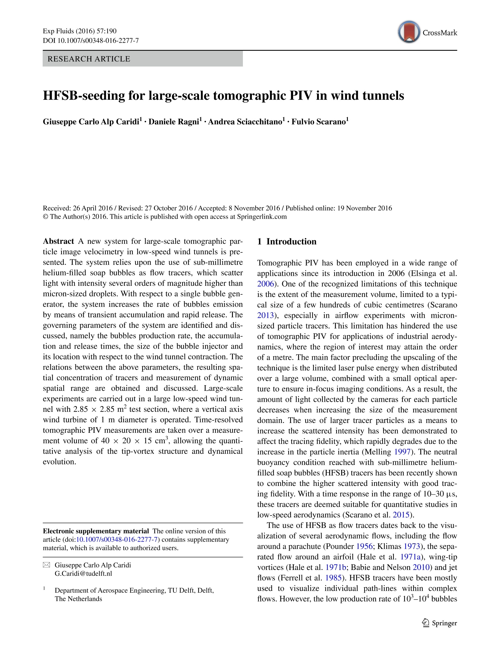
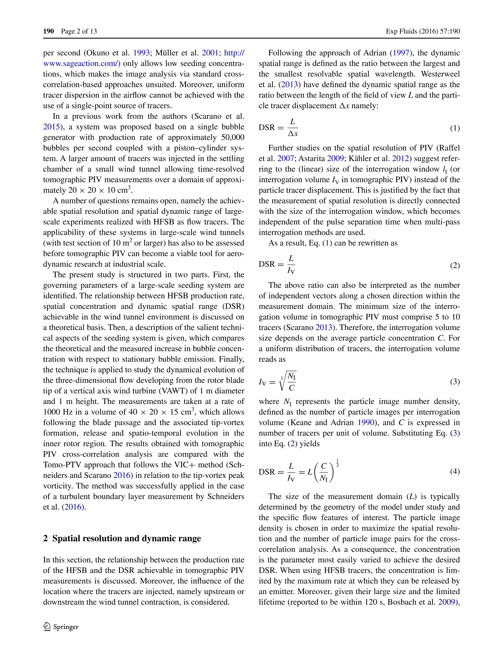
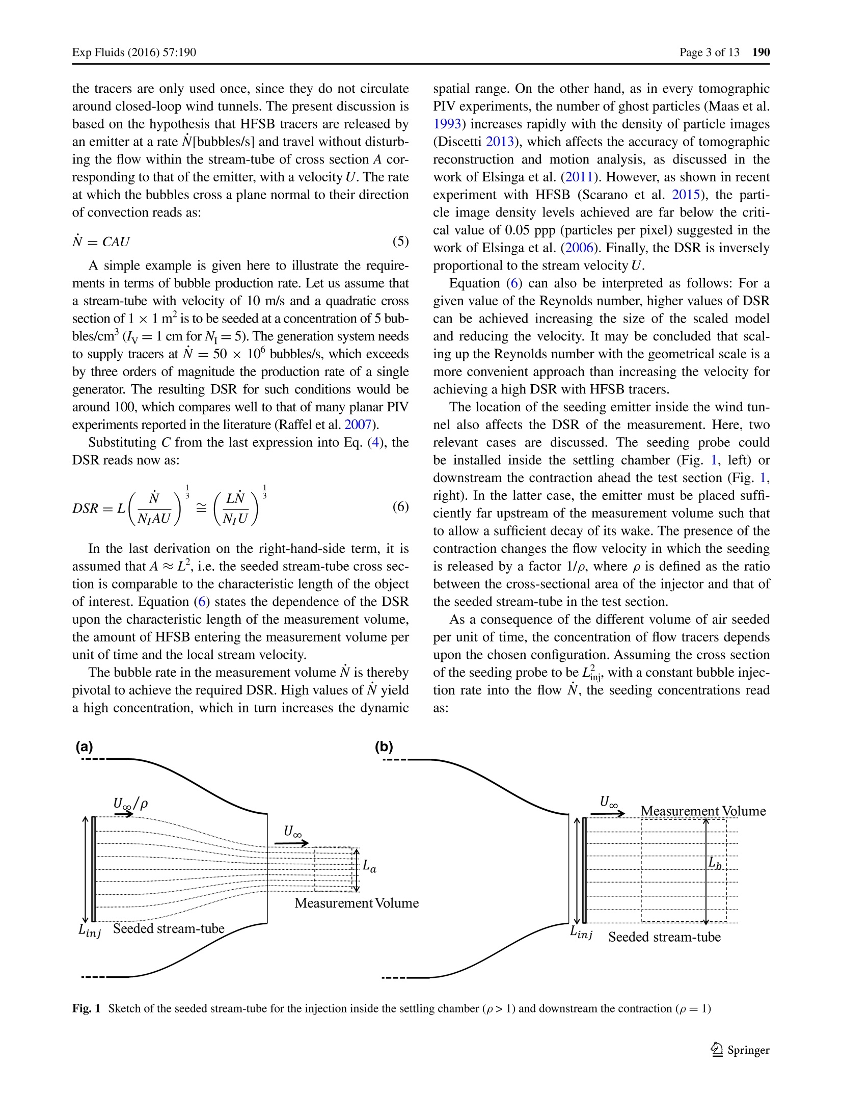
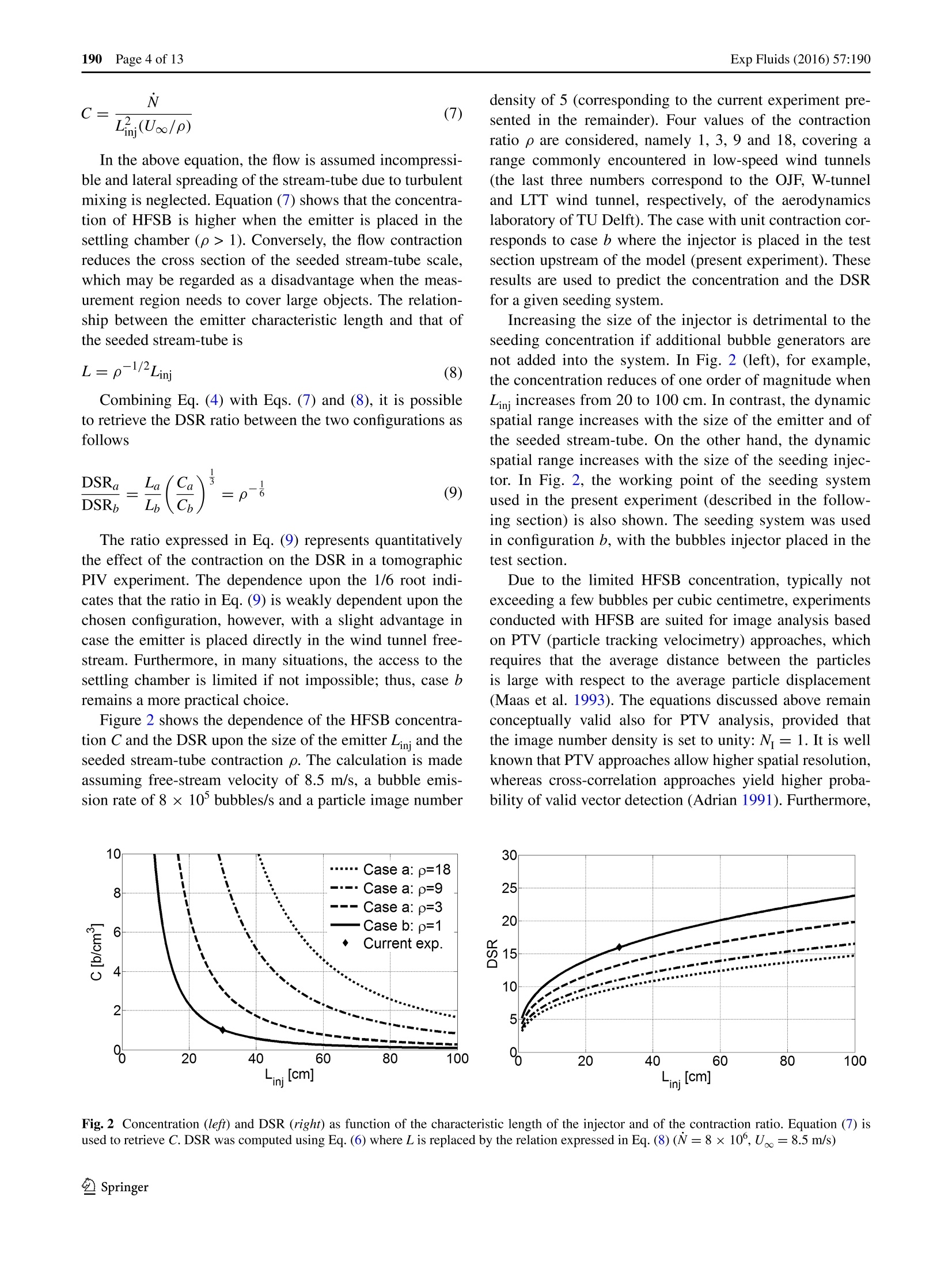
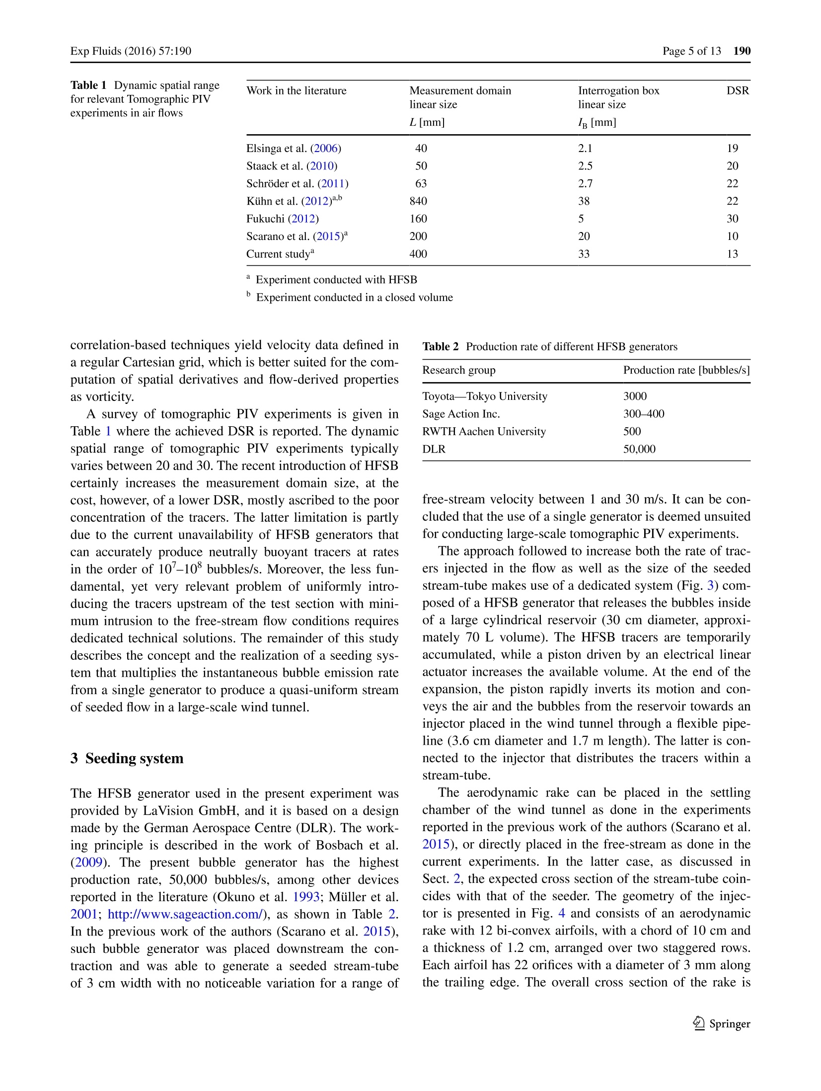
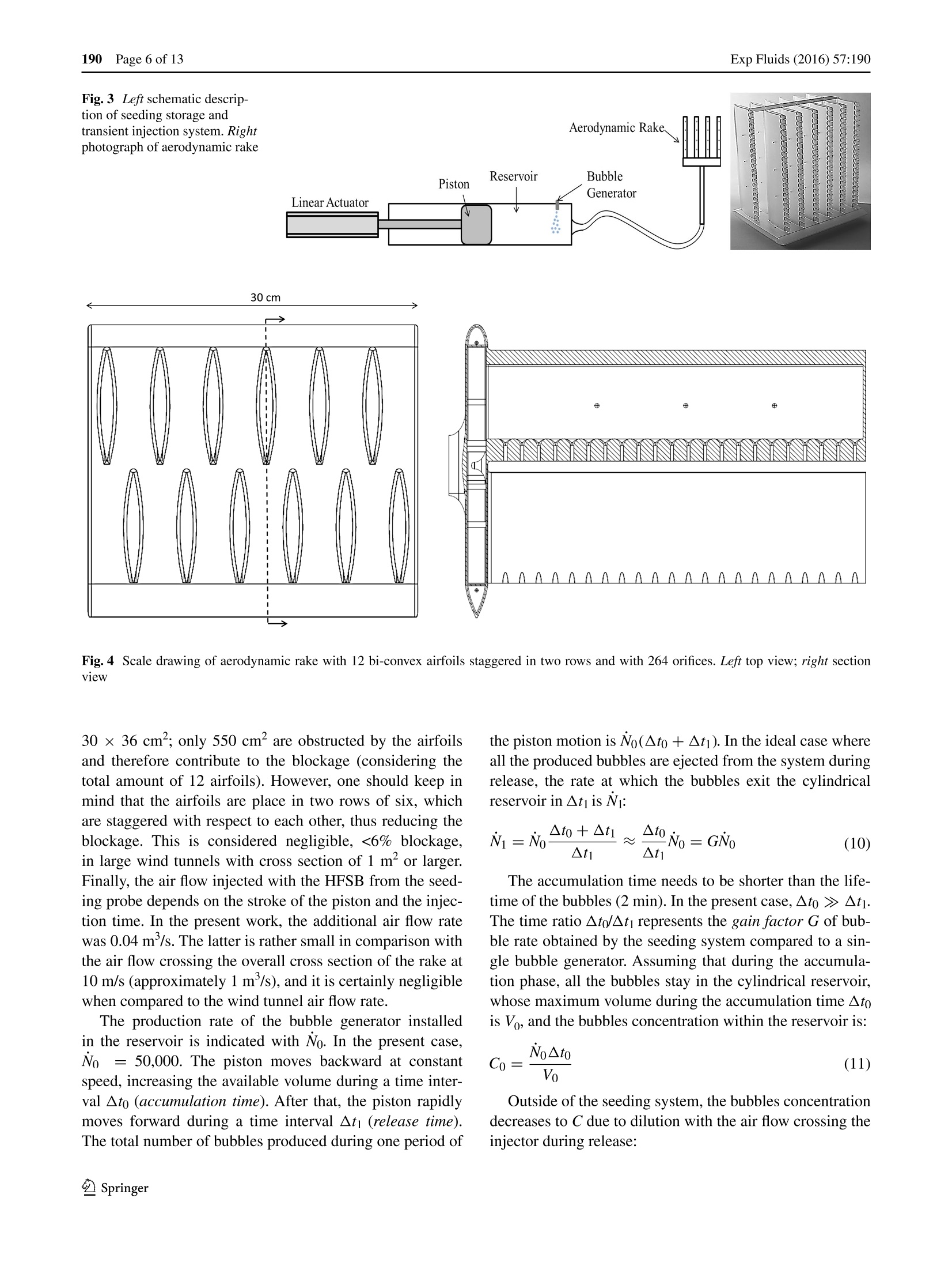
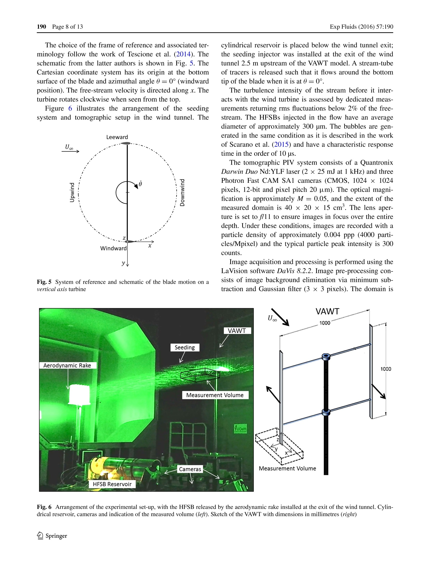
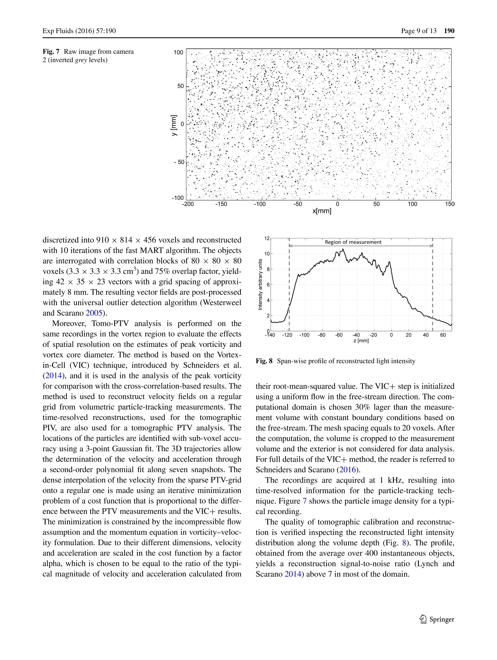
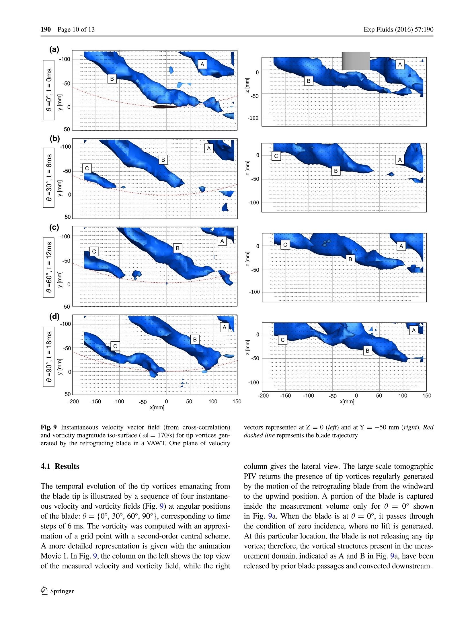
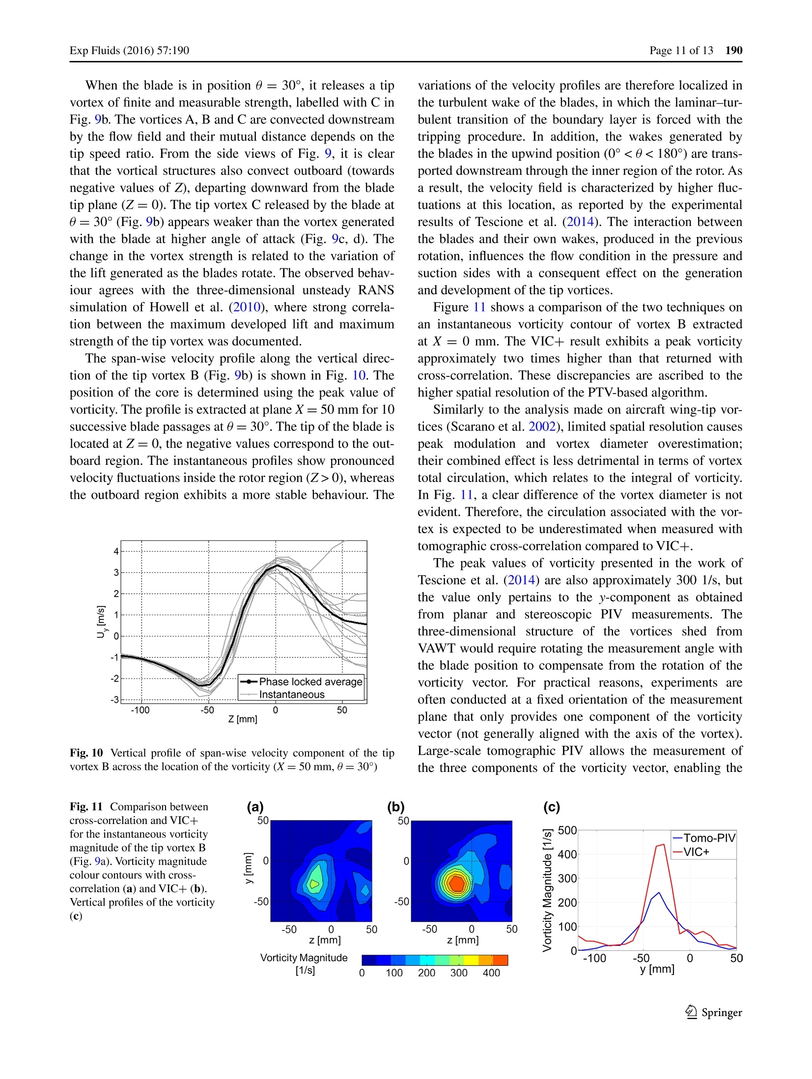
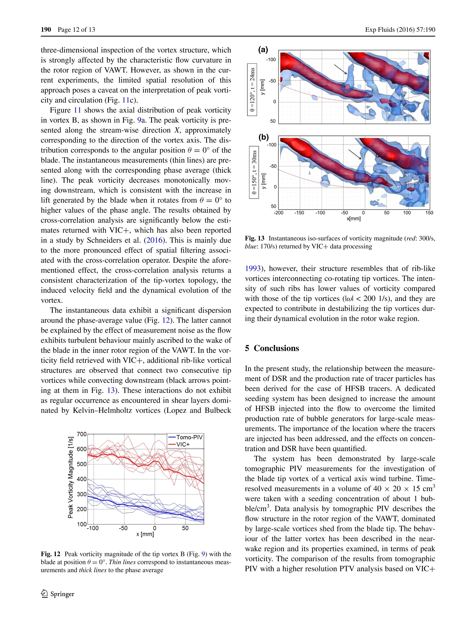
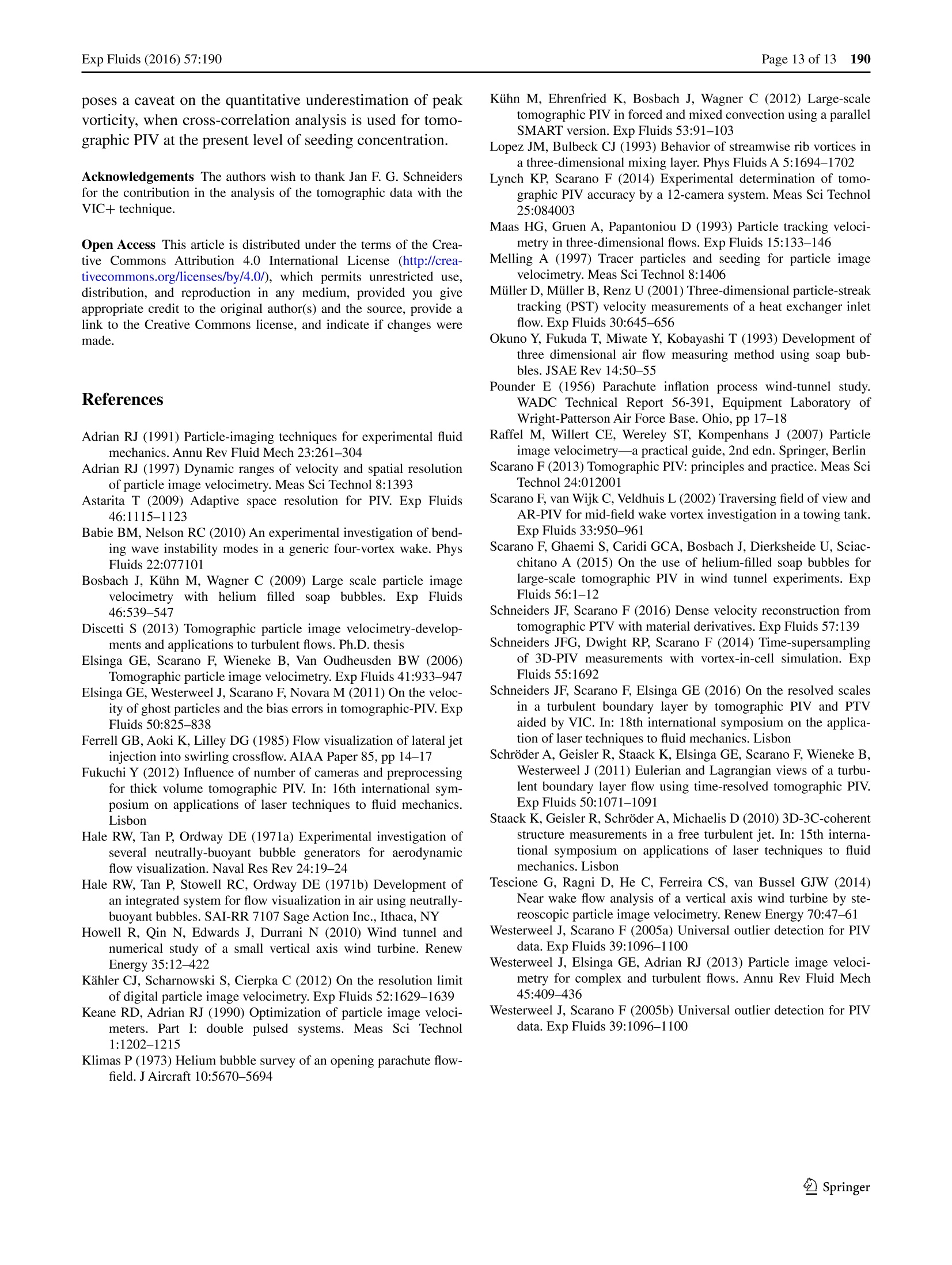
Exp Fluids (2016) 57：190DOI 10.1007/s00348-016-2277-7CrossMarkRESEARCH ARTICLE 190Exp Fluids (2016) 57：190Page 2 of 13 HFSB-seeding for large-scale tomographic PIV in wind tunnels Giuseppe Carlo Alp Caridi·Daniele Ragnil·Andrea Sciacchitanol·Fulvio Scaranol Received： 26 April 2016 / Revised： 27 October 2016/ Accepted： 8 November 2016/ Published online： 19 November 2016O The Author(s) 2016. This article is published with open access at Springerlink.com Abstract A new system for large-scale tomographic par-ticle image velocimetry in low-speed wind tunnels is pre-sented. The system relies upon the use of sub-millimetrehelium-filled soap bubbles as flow tracers， which scatterlight with intensity several orders of magnitude higher thanmicron-sized droplets. With respect to a single bubble gen-erator， the system increases the rate of bubbles emissionby means of transient accumulation and rapid release. Thegoverning parameters of the system are identified and dis-cussed， namely the bubbles production rate， the accumula-tion and release times， the size of the bubble injector andits location with respect to the wind tunnel contraction. Therelations between the above parameters， the resulting spa-tial concentration of tracers and measurement of dynamicspatial range are obtained and discussed. Large-scaleexperiments are carried out in a large low-speed wind tun-nel with 2.85×2.85 m²test section， where a vertical axiswind turbine of 1 m diameter is operated. Time-resolvedtomographic PIV measurements are taken over a measure-ment volume of 40 × 20 ×15 cm’， allowing the quanti-tative analysis of the tip-vortex structure and dynamicalevolution. Electronic supplementary material The online version of thisarticle (doi：10.1007/s00348-016-2277-7) contains supplementarymaterial， which is available to authorized users. 区Giuseppe Carlo Alp CaridiG.Caridi@tudelft.nl Department of Aerospace Engineering， TU Delft， Delft，The Netherlands 1 Introduction Tomographic PIV has been employed in a wide range ofapplications since its introduction in 2006 (Elsinga et al.2006). One of the recognized limitations of this techniqueis the extent of the measurement volume， limited to a typi-cal size of a few hundreds of cubic centimetres (Scarano2013)， especially in airflow experiments with micron-sized particle tracers. This limitation has hindered the useof tomographic PIV for applications of industrial aerody-namics， where the region of interest may attain the orderof a metre. The main factor precluding the upscaling of thetechnique is the limited laser pulse energy when distributedover a large volume， combined with a small optical aper-ture to ensure in-focus imaging conditions. As a result， theamount of light collected by the cameras for each particledecreases when increasing the size of the measurementdomain. The use of larger tracer particles as a means toincrease the scattered intensity has been demonstrated toaffect the tracing fidelity， which rapidly degrades due to theincrease in the particle inertia (Melling 1997). The neutralbuoyancy condition reached with sub-millimetre helium-filled soap bubbles (HFSB) tracers has been recently shownto combine the higher scattered intensity with good trac-ing fidelity. With a time response in the range of 10-30 ps，these tracers are deemed suitable for quantitative studies inlow-speed aerodynamics (Scarano et al. 2015). The use of HFSB as flow tracers dates back to the visu-alization of several aerodynamic flows， including the flowaround a parachute (Pounder 1956； Klimas 1973)， the sepa-rated flow around an airfoil (Hale et al. 1971a)， wing-tipvortices (Hale et al. 1971b； Babie and Nelson 2010) and jetflows (Ferrell et al. 1985). HFSB tracers have been mostlyused to visualize individual path-lines within complexflows. However， the low production rate of 10-10+ bubbles per second (Okuno et al. 1993；Muller et al. 2001； http：//www.sageaction.com/) only allows low seeding concentra-tions， which makes the image analysis via standard cross-correlation-based approaches unsuited. Moreover， uniformtracer dispersion in the airflow cannot be achieved with theuse of a single-point source of tracers. In a previous work from the authors (Scarano et al.2015)， a system was proposed based on a single bubblegenerator with production rate of approximately 50，000bubbles per second coupled with a piston-cylinder sys-tem. A larger amount of tracers was injected in the settlingchamber of a small wind tunnel allowing time-resolvedtomographic PIV measurements over a domain of approxi-mately 20 ×20×10 cm’. A number of questions remains open， namely the achiev-able spatial resolution and spatial dynamic range of large-scale experiments realized with HFSB as flow tracers. Theapplicability of these systems in large-scale wind tunnels(with test section of 10 m² or larger) has also to be assessedbefore tomographic PIV can become a viable tool for aero-dynamic research at industrial scale. The present study is structured in two parts. First， thegoverning parameters of a large-scale seeding system areidentified. The relationship between HFSB production rate，spatial concentration and dynamic spatial range (DSR)achievable in the wind tunnel environment is discussed ona theoretical basis. Then， a description of the salient techni-cal aspects of the seeding system is given， which comparesthe theoretical and the measured increase in bubble concen-tration with respect to stationary bubble emission. Finally，the technique is applied to study the dynamical evolution ofthe three-dimensional flow developing from the rotor bladetip of a vertical axis wind turbine (VAWT) of 1 m diameterand 1 m height. The measurements are taken at a rate of1000 Hz in a volume of 40 × 20 × 15 cm， which allowsfollowing the blade passage and the associated tip-vortexformation， release and spatio-temporal evolution in theinner rotor region. The results obtained with tomographicPIV cross-correlation analysis are compared with theTomo-PTV approach that follows the VIC+ method (Sch-neiders and Scarano 2016) in relation to the tip-vortex peakvorticity. The method was successfully applied in the caseof a turbulent boundary layer measurement by Schneiderset al. (2016). 2 Spatial resolution and dynamic range In this section， the relationship between the production rateof the HFSB and the DSR achievable in tomographic PIVmeasurements is discussed. Moreover， the influence of thelocation where the tracers are injected， namely upstream ordownstream the wind tunnel contraction， is considered. Following the approach of Adrian (1997)， the dynamicspatial range is defined as the ratio between the largest andthe smallest resolvable spatial wavelength. Westerweelet al. (2013) have defined the dynamic spatial range as theratio between the length of the field of view L and the parti-cle tracer displacement ▲x namely： Further studies on the spatial resolution of PIV (Raffelet al. 2007； Astarita 2009； Kahler et al.2012) suggest refer-ring to the (linear) size of the interrogation window l(orinterrogation volume ly in tomographic PIV) instead of theparticle tracer displacement. This is justified by the fact thatthe measurement of spatial resolution is directly connectedwith the size of the interrogation window， which becomesindependent of the pulse separation time when multi-passinterrogation methods are used. As a result， Eq. (1) can be rewritten as The above ratio can also be interpreted as the numberof independent vectors along a chosen direction within themeasurement domain. The minimum size of the interro-gation volume in tomographic PIV must comprise 5 to 10tracers (Scarano 2013). Therefore， the interrogation volumesize depends on the average particle concentration C. Fora uniform distribution of tracers， the interrogation volumereads as where N represents the particle image number density，defined as the number of particle images per interrogationvolume (Keane and Adrian 1990)， and C is expressed innumber of tracers per unit of volume. Substituting Eq. (3)into Eq.(2) yields The size of the measurement domain (L) is typicallydetermined by the geometry of the model under study andthe specific flow features of interest. The particle imagedensity is chosen in order to maximize the spatial resolu-tion and the number of particle image pairs for the cross-correlation analysis. As a consequence， the concentrationis the parameter most easily varied to achieve the desiredDSR. When using HFSB tracers， the concentration is lim-ited by the maximum rate at which they can be released byan emitter. Moreover， given their large size and the limitedlifetime (reported to be within 120 s， Bosbach et al. 2009)， the tracers are only used once， since they do not circulatearound closed-loop wind tunnels. The present discussion isbased on the hypothesis that HFSB tracers are released byan emitter at a rate N[bubbles/s] and travel without disturb-ing the flow within the stream-tube of cross section A cor-responding to that of the emitter， with a velocity U. The rateat which the bubbles cross a plane normal to their directionof convection reads as： A simple example is given here to illustrate the require-ments in terms of bubble production rate. Let us assume thata stream-tube with velocity of 10 m/s and a quadratic crosssection of 1× 1 m² is to be seeded at a concentration of 5 bub-bles/cm(Iy=1 cm for N=5). The generation system needsto supply tracers at N = 50×10° bubbles/s， which exceedsby three orders of magnitude the production rate of a singlegenerator. The resulting DSR for such conditions would bearound 100， which compares well to that of many planar PIVexperiments reported in the literature (Raffel et al. 2007). Substituting C from the last expression into Eq. (4)， theDSR reads now as： In the last derivation on the right-hand-side term， it isassumed that AL， i.e. the seeded stream-tube cross sec-tion is comparable to the characteristic length of the objectof interest. Equation (6) states the dependence of the DSRupon the characteristic length of the measurement volume，the amount of HFSB entering the measurement volume perunit of time and the local stream velocity. The bubble rate in the measurement volume N is therebypivotal to achieve the required DSR. High values of N yielda high concentration， which in turn increases the dynamic spatial range. On the other hand， as in every tomographicPIV experiments， the number of ghost particles (Maas et al.1993) increases rapidly with the density of particle images(Discetti 2013)， which affects the accuracy of tomographicreconstruction and motion analysis， as discussed in thework of Elsinga et al. (2011). However， as shown in recentexperiment with HFSB (Scarano et al. 2015)， the parti-cle image density levels achieved are far below the criti-cal value of 0.05 ppp (particles per pixel) suggested in thework of Elsinga et al. (2006). Finally， the DSR is inverselyproportional to the stream velocity U. Equation (6) can also be interpreted as follows： For agiven value of the Reynolds number， higher values of DSRcan be achieved increasing the size of the scaled modeland reducing the velocity. It may be concluded that scal-ing up the Reynolds number with the geometrical scale is amore convenient approach than increasing the velocity forachieving a high DSR with HFSB tracers. The location of the seeding emitter inside the wind tun-nel also affects the DSR of the measurement. Here， tworelevant cases are discussed. The seeding probe couldbe installed inside the settling chamber (Fig. 1， left) ordownstream the contraction ahead the test section (Fig. 1，right). In the latter case， the emitter must be placed suffi-ciently far upstream of the measurement volume such thatto allow a sufficient decay of its wake. The presence of thecontraction changes the flow velocity in which the seedingis released by a factor 1/p， where p is defined as the ratiobetween the cross-sectional area of the injector and that ofthe seeded stream-tube in the test section. As a consequence of the different volume of air seededper unit of time，the concentration of flow tracers dependsupon the chosen configuration. Assuming the cross sectionof the seeding probe to be Li， with a constant bubble injec-tion rate into the flow N， the seeding concentrations readas. Fig. 1 Sketch of the seeded stream-tube for the injection inside the settling chamber (p>1) and downstream the contraction (p=1) In the above equation， the flow is assumed incompressi-ble and lateral spreading of the stream-tube due to turbulentmixing is neglected. Equation (7) shows that the concentra-tion of HFSB is higher when the emitter is placed in thesettling chamber (p>1). Conversely， the flow contractionreduces the cross section of the seeded stream-tube scale，which may be regarded as a disadvantage when the meas-urement region needs to cover large objects. The relation-ship between the emitter characteristic length and that ofthe seeded stream-tube is Combining Eq. (4) with Eqs. (7) and (8)， it is possibleto retrieve the DSR ratio between the two configurations asfollows The ratio expressed in Eq. (9) represents quantitativelythe effect of the contraction on the DSR in a tomographicPIV experiment. The dependence upon the 1/6 root indi-cates that the ratio in Eq. (9) is weakly dependent upon thechosen configuration， however， with a slight advantage incase the emitter is placed directly in the wind tunnel free-stream. Furthermore， in many situations， the access to thesettling chamber is limited if not impossible； thus， case bremains a more practical choice. Figure 2 shows the dependence of the HFSB concentra-tion C and the DSR upon the size of the emitter Lini and theseeded stream-tube contraction p. The calculation is madeassuming free-stream velocity of 8.5 m/s， a bubble emis-sion rate of 8 ×10bubbles/s and a particle image number density of 5 (corresponding to the current experiment pre-sented in the remainder). Four values of the contractionratio p are considered， namely 1， 3， 9 and 18， covering arange commonly encountered in low-speed wind tunnels(the last three numbers correspond to the OJF， W-tunneland LTT wind tunnel， respectively， of the aerodynamicslaboratory of TU Delft). The case with unit contraction cor-responds to case b where the injector is placed in the testsection upstream of the model (present experiment). Theseresults are used to predict the concentration and the DSRfor a given seeding system. Increasing the size of the injector is detrimental to theseeding concentration if additional bubble generators arenot added into the system. In Fig. 2 (left)， for example，the concentration reduces of one order of magnitude whenLin increases from 20 to 100 cm. In contrast， the dynamicspatial range increases with the size of the emitter and ofthe seeded stream-tube. On the other hand， the dynamicspatial range increases with the size of the seeding injec-tor. In Fig. 2， the working point of the seeding systemused in the present experiment (described in the follow-ing section) is also shown. The seeding system was usedin configuration b， with the bubbles injector placed in thetest section. Due to the limited HFSB concentration， typically notexceeding a few bubbles per cubic centimetre， experimentsconducted with HFSB are suited for image analysis basedon PTV (particle tracking velocimetry) approaches， whichrequires that the average distance between the particlesis large with respect to the average particle displacement(Maas et al. 1993). The equations discussed above remainconceptually valid also for PTV analysis， provided thatthe image number density is set to unity： N= 1. It is wellknown that PTV approaches allow higher spatial resolution，whereas cross-correlation approaches yield higher proba-bility of valid vector detection (Adrian 1991). Furthermore， Fig. 2 Concentration (left) and DSR (right) as function of the characteristic length of the injector and of the contraction ratio. Equation (7) isused to retrieve C. DSR was computed using Eq. (6) where L is replaced by the relation expressed in Eq. (8)(N=8×10， U。=8.5 m/s) Table 1 Dynamic spatial range for relevant Tomographic PIV experiments in air flows Work in the literature Measurement domain Interrogation box DSR linear size linear size L[mm] B [mm] Elsinga et al. (2006) 19 Staack et al.(2010) Schroder et al. (2011) Kuhn et al. (2012)a， 840 22 Fukuchi (2012) 160 5 30 Scarano et al. (2015) 200 20 10 Current study" 400 33 13 Experiment conducted with HFSB Experiment conducted in a closed volume correlation-based techniques yield velocity data defined ina regular Cartesian grid， which is better suited for the com-putation of spatial derivatives and flow-derived propertiesas vorticity. A survey of tomographic PIV experiments is given inTable 1 where the achieved DSR is reported. The dynamicspatial range of tomographic PIV experiments typicallyvaries between 20 and 30. The recent introduction of HFSBcertainly increases the measurement domain size， at thecost， however， of a lower DSR， mostly ascribed to the poorconcentration of the tracers. The latter limitation is partlydue to the current unavailability of HFSB generators thatcan accurately produce neutrally buoyant tracers at ratesin the order of 10'-10° bubbles/s.Moreover， the less fun-damental， yet very relevant problem of uniformly intro-ducing the tracers upstream of the test section with mini-mum intrusion to the free-stream flow conditions requiresdedicated technical solutions. The remainder of this studydescribes the concept and the realization of a seeding sys-tem that multiplies the instantaneous bubble emission ratefrom a single generator to produce a quasi-uniform streamof seeded flow in a large-scale wind tunnel. 3 Seeding system The HFSB generator used in the present experiment wasprovided by LaVision GmbH， and it is based on a designmade by the German Aerospace Centre (DLR). The work-ing principle is described in the work of Bosbach et al.(2009). The present bubble generator has the highestproduction rate， 50，000 bubbles/s， among other devicesreported in the literature (Okuno et al. 1993； Muller et al.2001； http：//www.sageaction.com/)， as shown in Table 2.In the previous work of the authors (Scarano et al. 2015)，such bubble generator was placed downstream the con-traction and was able to generate a seeded stream-tubeof 3 cm width with no noticeable variation for a range of Table 2 Production rate of different HFSB generators Research group Production rate [bubbles/s] Toyota—Tokyo University 3000 Sage Action Inc. 300-400 RWTH Aachen University 500 DLR 50，000 free-stream velocity between 1 and 30 m/s. It can be con-cluded that the use of a single generator is deemed unsuitedfor conducting large-scale tomographic PIV experiments The approach followed to increase both the rate of trac-ers injected in the flow as well as the size of the seededstream-tube makes use of a dedicated system (Fig. 3) com-posed of a HFSB generator that releases the bubbles insideof a large cylindrical reservoir (30 cm diameter， approxi-mately 70 L volume). The HFSB tracers are temporarilyaccumulated， while a piston driven by an electrical linearactuator increases the available volume. At the end of theexpansion， the piston rapidly inverts its motion and con-veys the air and the bubbles from the reservoir towards aninjector placed in the wind tunnel through a flexible pipe-line (3.6 cm diameter and 1.7 m length). The latter is con-nected to the injector that distributes the tracers within astream-tube. . The aerodynamic rake can be placed in the settlingchamber of the wind tunnel as done in the experimentsreported in the previous work of the authors (Scarano et al.2015)， or directly placed in the free-stream as done in thecurrent experiments. In the latter case， as discussed inSect. 2， the expected cross section of the stream-tube coin-cides with that of the seeder. The geometry of the injec-tor is presented in Fig. 4 and consists of an aerodynamicrake with 12 bi-convex airfoils， with a chord of 10 cm anda thickness of 1.2 cm， arranged over two staggered rows.Each airfoil has 22 orifices with a diameter of 3 mm alongthe trailing edge. The overall cross section of the rake is 30 cm Fig.4 Scale drawing of aerodynamic rake with 12 bi-convex airfoils staggered in two rows and with 264 orifices. Left top view；right sectionview 30 × 36 cm²； only 550 cm’ are obstructed by the airfoilsand therefore contribute to the blockage (considering thetotal amount of 12 airfoils). However， one should keep inmind that the airfoils are place in two rows of six， whichare staggered with respect to each other， thus reducing theblockage. This is considered negligible， <6% blockage，in large wind tunnels with cross section of 1 m² or larger.Finally， the air flow injected with the HFSB from the seed-ing probe depends on the stroke of the piston and the injec-tion time. In the present work， the additional air flow ratewas 0.04 m’/s.The latter is rather small in comparison withthe air flow crossing the overall cross section of the rake at10 m/s (approximately 1 m’/s)， and it is certainly negligiblewhen compared to the wind tunnel air flow rate. The production rate of the bubble generator installedin the reservoir is indicated with No. In the present case，No= 50，000. The piston moves backward at constantspeed， increasing the available volume during a time interval ▲to (accumulation time). After that， the piston rapidlymoves forward during a time interval At(release time).The total number of bubbles produced during one period of the piston motion is No(to+At ). In the ideal case whereall the produced bubbles are ejected from the system duringrelease， the rate at which the bubbles exit the cylindricalreservoir in ▲t is N： The accumulation time needs to be shorter than the life-time of the bubbles (2 min). In the present case， Ato >Atj.The time ratio Ato/At represents the gain factor G of bub-ble rate obtained by the seeding system compared to a sin-gle bubble generator. Assuming that during the accumula-tion phase， all the bubbles stay in the cylindrical reservoir，whose maximum volume during the accumulation time Atois Vo， and the bubbles concentration within the reservoir is： Outside of the seeding system， the bubbles concentrationdecreases to C due to dilution with the air flow crossing theinjector during release： Vw is the air volume flowing through the diffuser andin which the bubbles are ejected. The term Vwt can beexpressed as： where u is the velocity of the flow in which the HFSB areinjected and is equal to Up in case a (injector in the set-tling chamber) and U. in case b (injector in the test section； see Sect. 2). Substituting Eq. (13) into Eq. (12) andmaking use of the definition of the gain factor， the expres-sion of the concentration becomes： Equation (14) shows the dependence of the concentra-tion from the main working parameters of the seeding sys-tem. The choice of the bubble generator determines thebubbles production rate， No， and therefore is crucial for theoptimization of C. The latter is directly dependent upon thegain factor， which is varied by changing the accumulationtime ▲to， provided it does not exceed the bubbles lifetime.The cross section of the seeded stream-tube A， determinesthe air volume flow rate where the bubbles are releasedand therefore the dilution in the wind tunnel. Increasing Areduces the concentration of tracers. Using Eq. (14) with the values in Table 3， correspondingto the experiment described in the next section， a theoreti-cal concentration (Cth) of 3 bubbles/cm’ is expected. Thisconcentration allows tomographic PIV measurements toinvestigate flow structures of the order of a few centime-tres， as it will be done in the next section for the analysisof the blade tip vortex of a vertical axis wind turbine. Theconcentration observed within the measurements (Cmeas)is considerably less than the above one (1 bubble/cm) asshown in Fig. 2， left. This difference is ascribed to a num-ber of factors， most importantly， bubbles extinction duringtheir transport from the reservoir to the exit of the injec-tor and bubble collisions inside the reservoir. As a resultof the lower concentration， the tomographic PIV analysis is conducted with larger interrogation windows， yielding inturn a lower spatial resolution. Concluding， it was noticed that the loss of bubblesupstream of the injector poses some limits to the seed-ing system described above. A possible solution to complywith this issue will be the use of many bubble generators inparallel installed inside the wind tunnel. A multi-generatorsystem allows producing HFSB directly in the stream ofthe wind tunnel without transport losses and introduction ofthe air volume V. The latter alternative， however， requiresa large number of nozzles， on the order of G for a givenNo = 50，000 in order to retrieve the same concentration andDSR obtained for the present seeding system. Although amulti-generator system is not yet available at present time，the analysis performed in the present section can be extendedto the latter case， provided that a unitary gain factor (G=1)and the total production rate of all nozzles are considered. 4 Wind tunnel experiment The above described system is used to perform time-resolved tomographic PIV measurements ona scaledmodel of vertical axis wind turbine (VAWT). The meas-urements are taken in the Open Jet Facility (OJF) of TUDelft. The wind tunnel features an open test section withclosed-circuit. At the end of the contraction， the wind tun-nel has an octagonal cross section of 2.85 ×2.85 m. Theair flow is driven by a 500 kW electric motor. In the testsection， the free-stream velocity can range from 3 to 35 m/swith a maximum turbulence intensity of 0.5%. The modelis a two-blade H-shaped rotor VAWT of 1 m diameter (D).The rotor blades are shaped following the NACA0018 pro-file with 6 cm chord length and installed with zero angleof attack. The blades are tripped by zig-zag stripes in orderto force the boundary layer transition from laminar to tur-bulent regime and avoid the occurrence of laminar sepa-ration bubbles. The blade span H is 1 m long， yielding anaspect ratio AR =HID =1. Measurements are taken atfree-stream velocity U= 8.5 m/s and rotational speed2=800 rpm， yielding a tip speed ratio 入= 5. The Reyn-olds number based on the chord length and the tangentialvelocity of the blades is Ree=170，000. Table 3 Theoretical and measured bubble concentration for the VAWT experiment No (b/s) Ato (s) ▲tj (s) G Vo (cm’) A (cm²) U (m/s) 50，000 50 1 50 16，000 .900 8.5 Cth (b/cm) Cmeas (b/cm’) DSRh DSR 'meas 3 1 28 13 The choice of the frame of reference and associated ter-minology follow the work of Tescione et al. (2014). Theschematic from the latter authors is shown in Fig. 5. TheCartesian coordinate system has its origin at the bottomsurface of the blade and azimuthal angle 0=0°(windwardposition). The free-stream velocity is directed along x. Theturbine rotates clockwise when seen from the top. Figure 6 illustrates the arrangement of the seedingsystem and tomographic setup in the wind tunnel. The Fig.5 System of reference and schematic of the blade motion on avertical axis turbine cylindrical reservoir is placed below the wind tunnel exit；the seeding injector was installed at the exit of the windtunnel 2.5 m upstream of the VAWT model. A stream-tubeof tracers is released such that it flows around the bottomtip of the blade when it is at0=0°. The turbulence intensity of the stream before it inter-acts with the wind turbine is assessed by dedicated meas-urements returning rms fluctuations below 2% of the free-stream. The HFSBs injected in the flow have an averagediameter of approximately 300 um. The bubbles are gen-erated in the same condition as it is described in the workof Scarano et al. (2015) and have a characteristic responsetime in the order of 10 us. The tomographic PIV system consists of a QuantronixDarwin Duo Nd：YLF laser (2x 25 mJ at 1 kHz) and threePhotron Fast CAM SA1 cameras (CMOS， 1024 × 1024pixels， 12-bit and pixel pitch 20 um). The optical magni-fication is approximately M=0.05， and the extent of themeasured domain is 40 × 20 × 15 cm’. The lens aper-ture is set to f/11 to ensure images in focus over the entiredepth. Under these conditions， images are recorded with aparticle density of approximately 0.004 ppp(4000 parti-cles/Mpixel) and the typical particle peak intensity is 300counts. Image acquisition and processing is performed using theLaVision software DaVis 8.2.2. Image pre-processing con-sists of image background elimination via minimum sub-traction and Gaussian filter (3×3 pixels). The domain is Fig.6 Arrangement of the experimental set-up， with the HFSB released by the aerodynamic rake installed at the exit of the wind tunnel. Cylin-drical reservoir， cameras and indication of the measured volume (left). Sketch of the VAWT with dimensions in millimetres (right) Fig. 7 Raw image from camera2 (inverted grey levels) discretized into 910×814x456 voxels and reconstructedwith 10 iterations of the fast MART algorithm. The objectsare interrogated with correlation blocks of 80 ×80 × 80voxels (3.3×3.3×3.3 cm) and 75% overlap factor， yield-ing 42 × 35 ×23 vectors with a grid spacing of approxi-mately 8 mm. The resulting vector fields are post-processedwith the universal outlier detection algorithm (Westerweeland Scarano 2005). Moreover， Tomo-PTV analysis is performed on thesame recordings in the vortex region to evaluate the effectsof spatial resolution on the estimates of peak vorticity andvortex core diameter. The method is based on the Vortex-in-Cell (VIC) technique， introduced by Schneiders et al.(2014)， and it is used in the analysis of the peak vorticityfor comparison with the cross-correlation-based results. Themethod is used to reconstruct velocity fields on a regulargrid from volumetric particle-tracking measurements. Thetime-resolved reconstructions， used for the tomographicPIV， are also used for a tomographic PTV analysis. Thelocations of the particles are identified with sub-voxel accu-racy using a 3-point Gaussian fit. The 3D trajectories allowthe determination of the velocity and acceleration througha second-order polynomial fit along seven snapshots. Thedense interpolation of the velocity from the sparse PTV-gridonto a regular one is made using an iterative minimizationproblem of a cost function that is proportional to the differ-ence between the PTV measurements and the VIC+ results.The minimization is constrained by the incompressible flowassumption and the momentum equation in vorticity-veloc-ity formulation. Due to their different dimensions，velocityand acceleration are scaled in the cost function by a factoralpha， which is chosen to be equal to the ratio of the typi-cal magnitude of velocity and acceleration calculated from Fig. 8 Span-wise profile of reconstructed light intensity their root-mean-squared value. The VIC+ step is initializedusing a uniform flow in the free-stream direction. The com-putational domain is chosen 30% lager than the measure-ment volume with constant boundary conditions based onthe free-stream. The mesh spacing equals to 20 voxels. Afterthe computation， the volume is cropped to the measurementvolume and the exterior is not considered for data analysis.For full details of the VIC+ method， the reader is referred toSchneiders and Scarano (2016). The recordings are acquired at 1 kHz， resulting intotime-resolved information for the particle-tracking tech-nique. Figure 7 shows the particle image density for a typi-cal recording. The quality of tomographic calibration and reconstruc-tion is verified inspecting the reconstructed light intensitydistribution along the volume depth (Fig. 8). The profile，obtained from the average over 400 instantaneous objects，yields a reconstruction signal-to-noise ratio (Lynch andScarano 2014) above 7 in most of the domain. (a) x[mm]n] 4.1 Results The temporal evolution of the tip vortices emanating fromthe blade tip is illustrated by a sequence of four instantane-ous velocity and vorticity fields (Fig. 9)at angular positionsof the blade： 0={0°， 30°， 60°， 90°}， corresponding to timesteps of 6 ms. The vorticity was computed with an approxi-mation of a grid point with a second-order central scheme.A more detailed representation is given with the animationMovie 1. In Fig. 9， the column on the left shows the top viewof the measured velocity and vorticity field， while the right column gives the lateral view. The large-scale tomographicPIV returns the presenceof tip vortices regularly generatedby the motion of the retrograding blade from the windwardto the upwind position. A portion of the blade is capturedinside the measurement volume only for 0=0° shownin Fig. 9a. When the blade is at 0=0°， it passes throughthe condition of zero incidence， where no lift is generated.At this particular location， the blade is not releasing any tipvortex； therefore， the vortical structures present in the meas-urement domain， indicated as A and B in Fig. 9a， have beenreleased by prior blade passages and convected downstream. When the blade is in position 0= 30°， it releases a tipvortex of finite and measurable strength， labelled with C inFig. 9b. The vortices A， B and C are convected downstreamby the flow field and their mutual distance depends on thetip speed ratio. From the side views of Fig. 9， it is clearthat the vortical structures also convect outboard (towardsnegative values of Z)， departing downward from the bladetip plane (Z=0). The tip vortex C released by the blade at0=30°(Fig. 9b) appears weaker than the vortex generatedwith the blade at higher angle of attack (Fig. 9c，d). Thechange in the vortex strength is related to the variation ofthe lift generated as the blades rotate. The observed behav-iour agrees with the three-dimensional unsteady RANSsimulation of Howell et al. (2010)， where strong correla-tion between the maximum developed lift and maximumstrength of the tip vortex was documented. The span-wise velocity profile along the vertical direc-tion of the tip vortex B (Fig. 9b) is shown in Fig. 10. Theposition of the core is determined using the peak value ofvorticity. The profile is extracted at plane X= 50 mm for 10successive blade passages at 0=30°. The tip of the blade islocated at Z= 0， the negative values correspond to the out-board region. The instantaneous profiles show pronouncedvelocity fluctuations inside the rotor region (Z>0)， whereasthe outboard region exhibits a more stable behaviour. The Fig. 10 Vertical profile of span-wise velocity component of the tipvortex B across the location of the vorticity (X=50 mm，0=30°) variations of the velocity profiles are therefore localized inthe turbulent wake of the blades， in which the laminar-tur-bulent transition of the boundary layer is forced with thetripping procedure. In addition， the wakes generated bythe blades in the upwind position (0°<0<180°) are trans-ported downstream through the inner region of the rotor. Asa result， the velocity field is characterized by higher fluc-tuations at this location， as reported by the experimentalresults of Tescione et al. (2014). The interaction betweenthe blades and their own wakes， produced in the previousrotation， influences the flow condition in the pressure andsuction sides with a consequent effect on the generationand development of the tip vortices. Figure 11 shows a comparison of the two techniques onan instantaneous vorticity contour of vortex B extractedat X= 0 mm. The VIC+ result exhibits a peak vorticityapproximately two times higher than that returned withcross-correlation. These discrepancies are ascribed to thehigher spatial resolution of the PTV-based algorithm. Similarly to the analysis made on aircraft wing-tip vor-tices (Scarano et al. 2002)， limited spatial resolution causespeak modulation and vortex diameter overestimation：their combined effect is less detrimental in terms of vortextotal circulation， which relates to the integral of vorticity.In Fig. 11， a clear difference of the vortex diameter is notevident. Therefore， the circulation associated with the vor-tex is expected to be underestimated when measured withtomographic cross-correlation compared to VIC+. The peak values of vorticity presented in the work ofTescione et al. (2014) are also approximately 300 1/s， butthe value only pertains to the y-component as obtainedfrom planar and stereoscopic PIV measurements. Thethree-dimensional structure of the vortices shed fromVAWT would require rotating the measurement angle withthe blade position to compensate from the rotation of thevorticity vector. For practical reasons， experiments areoften conducted at a fixed orientation of the measurementplane that only provides one component of the vorticityvector (not generally aligned with the axis of the vortex).Large-scale tomographic PIV allows the measurement ofthe three components of the vorticity vector， enabling the Fig. 11 Comparison betweencross-correlation and VIC+for the instantaneous vorticitymagnitude of the tip vortex B(Fig.9a). Vorticity magnitudecolour contours with cross-correlation (a) and VIC+ (b).Vertical profiles of the vorticity(c) three-dimensional inspection of the vortex structure， whichis strongly affected by the characteristic flow curvature inthe rotor region of VAWT. However， as shown in the cur-rent experiments， the limited spatial resolution of thisapproach poses a caveat on the interpretation of peak vorti-city and circulation (Fig. 11c). Figure 11 shows the axial distribution of peak vorticityin vortex B， as shown in Fig. 9a. The peak vorticity is pre-sented along the stream-wise direction X， approximatelycorresponding to the direction of the vortex axis. The dis-tribution corresponds to the angular position 0=0°of theblade. The instantaneous measurements (thin lines) are pre-sented along with the corresponding phase average (thickline). The peak vorticity decreases monotonically mov-ing downstream， which is consistent with the increase inlift generated by the blade when it rotates from0=0° tohigher values of the phase angle. The results obtained bycross-correlation analysis are significantly below the esti-mates returned with VIC+， which has also been reportedin a study by Schneiders et al. (2016). This is mainly dueto the more pronounced effect of spatial filtering associ-ated with the cross-correlation operator. Despite the afore-mentioned effect， the cross-correlation analysis returns aconsistent characterization of the tip-vortex topology， theinduced velocity field and the dynamical evolution of thevortex. The instantaneous data exhibit a significant dispersionaround the phase-average value (Fig. 12). The latter cannotbe explained by the effect of measurement noise as the flowexhibits turbulent behaviour mainly ascribed to the wake ofthe blade in the inner rotor region of the VAWT. In the vor-ticity field retrieved with VIC+， additional rib-like vorticalstructures are observed that connect two consecutive tipvortices while convecting downstream (black arrows point-ing at them in Fig. 13). These interactions do not exhibitas regular occurrence as encountered in shear layers domi-nated by Kelvin-Helmholtz vortices (Lopez and Bulbeck Fig. 12 Peak vorticity magnitude of the tip vortex B (Fig.9) with theblade at position 0=0°. Thin lines correspond to instantaneous meas-urements and thick lines to the phase average Fig. 13 Instantaneous iso-surfaces of vorticity magnitude (red：300/s，blue： 170/s) returned by VIC+ data processing 1993)， however， their structure resembles that of rib-likevortices interconnecting co-rotating tip vortices. The inten-sity of such ribs has lower values of vorticity comparedwith those of the tip vortices (lωl <200 1/s)， and they areexpected to contribute in destabilizing the tip vortices dur-ing their dynamical evolution in the rotor wake region. 5 Conclusions In the present study， the relationship between the measure-ment of DSR and the production rate of tracer particles hasbeen derived for the case of HFSB tracers. A dedicatedseeding system has been designed to increase the amountof HFSB injected into the flow to overcome the limitedproduction rate of bubble generators for large-scale meas-urements. The importance of the location where the tracersare injected has been addressed， and the effects on concen-tration and DSR have been quantified. The system has been demonstrated by large-scaletomographic PIV measurements for the investigation ofthe blade tip vortex of a vertical axis wind turbine. Time-resolved measurements in a volume of 40 ×20x15 cm²were taken with a seeding concentration of about 1 bub-ble/cm’. Data analysis by tomographic PIV describes theflow structure in the rotor region of the VAWT，dominatedby large-scale vortices shed from the blade tip. The behav-iour of the latter vortex has been described in the near-wake region and its properties examined， in terms of peakvorticity. The comparison of the results from tomographicPIV with a higher resolution PTV analysis based on VIC+ poses a caveat on the quantitative underestimation of peakvorticity， when cross-correlation analysis is used for tomo-graphic PIV at the present level of seeding concentration. Acknowledgements The authors wish to thank Jan F. G. Schneidersfor the contribution in the analysis of the tomographic data with theVIC+ technique. Open Access This article is distributed under the terms of the Crea-tive Commons Attribution 4.0 International License (http：//crea-tivecommons.org/licenses/by/4.0/)， which permits unrestricted use，distribution， and reproduction in any medium， provided you giveappropriate credit to the original author(s) and the source， provide alink to the Creative Commons license， and indicate if changes weremade. References Adrian RJ (1991) Particle-imaging techniques for experimental fluidmechanics. Annu Rev Fluid Mech 23：261-304 Adrian RJ (1997) Dynamic ranges of velocity and spatial resolutionof particle image velocimetry. Meas Sci Technol 8：1393 Astarita T(2009) Adaptive space resolution for PIV. Exp Fluids46：1115-1123 Babie BM， Nelson RC (2010) An experimental investigation of bend-ing wave instability modes in a generic four-vortex wake. PhysFluids 22：077101 Bosbach J， Kuhn M. Wagner C (2009) Large scale particle imagevelocimetrywithn helium filled soap bubbles. Exp Fluids46：539-547 Discetti S (2013) Tomographic particle image velocimetry-develop-ments and applications to turbulent flows. Ph.D. thesis Elsinga GE， Scarano F， Wieneke B， Van Oudheusden BW (2006)Tomographic particle image velocimetry. Exp Fluids 41：933-947 Elsinga GE， Westerweel J， Scarano F， Novara M (2011) On the veloc-ity of ghost particles and the bias errors in tomographic-PIV. ExpFluids 50：825-838 Ferrell GB， Aoki K， Lilley DG (1985) Flow visualization of lateral jetinjection into swirling crossflow. AIAA Paper 85， pp 14-17 ( Fukuchi Y (2012) Influence of number of cameras and preprocessing for thick volume t o mographic PIV. In： 16t h int e rnational sym- posium o n applications of laser techniques to fl u id mechanics.Lisbon ) ( Hale R W， Tan P ， Ordway DE (19 7 1a) Exp e rimental inv e stigation ofseveral neutrally-buoyant bubble generators f or a erodynamic flow visualization. Naval Res Rev 24：19-24 ) ( Hale RW， T an P， Stowell RC， Ordway DE (1971b) Development ofan integrated system for flow vi s ualization in air using neutrally-buoyant bubbles. S AI-RR 7107 Sa g e Action Inc.， Ithaca， NY ) ( Howell R ， Qin N ， Edwards J， Durrani N (2010) Wind tunnel andnumerical s tudy of a small v e rtical a xis w ind turbine. R enew Energy 35：12-422 ) Kahler CJ， Scharnowski S， Cierpka C (2012) On the resolution limitof digital particle image velocimetry. Exp Fluids 52：1629-1639 Keane RD， Adrian RJ (1990) Optimization of particle image veloci-meters. Part I： double pulsed systems. Meas Sci Technol1：1202-1215 Klimas P (1973) Helium bubble survey of an opening parachute flow-field. J Aircraft 10：5670-5694 Kiihn M， Ehrenfried K， Bosbach J， Wagner C (2012) Large-scaletomographic PIV in forced and mixed convection using a parallelSMART version. Exp Fluids 53：91-103 Lopez JM， Bulbeck CJ (1993) Behavior ofstreamwise rib vortices ina three-dimensional mixing layer. Phys Fluids A 5：1694-1702 Lynch KP， Scarano F (2014) Experimental determination of tomo-graphic PIV accuracy by a 12-camera system. Meas Sci Technol25：084003 Maas HG， Gruen A， Papantoniou D (1993) Particle tracking veloci-metry in three-dimensional flows. Exp Fluids 15：133-146 Melling A (1997) Tracer particles and seeding for particle imagevelocimetry. Meas Sci Technol 8：1406 Muller D，Miiller B， Renz U (2001) Three-dimensional particle-streaktracking (PST) velocity measurements of a heat exchanger inletflow. Exp Fluids 30：645-656 Okuno Y， Fukuda T， Miwate Y， Kobayashi T (1993) Development ofthree dimensional air flow measuring method using soap bub-bles. JSAE Rev 14：50-55 Pounder E (1956) Parachute inflation process wind-tunnel study.WADC Technical Report 56-391， Equipment Laboratory ofWright-Patterson Air Force Base. Ohio， pp 17-18 Raffel M， Willert CE， Wereley ST， Kompenhans J (2007) Particle image velocimetry-a practical guide， 2nd edn. Springer， BerlinScarano F (2013) Tomographic PIV： principles and practice. Meas SciTechnol 24：012001 Scarano F， van Wijk C， Veldhuis L(2002) Traversing field of view andAR-PIV for mid-field wake vortex investigation in a towing tank.Exp Fluids 33：950-961 Scarano F， Ghaemi S， Caridi GCA， Bosbach J， Dierksheide U， Sciac-chitano A (2015) On the use of helium-filled soap bubbles forlarge-scale tomographic PIV in wind tunnel experiments. ExpFluids 56：1-12 Schneiders JF， Scarano F (2016) Dense velocity reconstruction fromtomographic PTV with material derivatives. Exp Fluids 57：139 Schneiders JFG， Dwight RP， Scarano F (2014) Time-supersamplingof 3D-PIV measurements with vortex-in-cell simulation. ExpFluids 55：1692 Schneiders JF， Scarano F， Elsinga GE (2016) On the resolved scalesin a turbulent boundary layer by tomographic PIV and PTVaided by VIC. In： 18th international symposium on the applica-tion of laser techniques to fluid mechanics. Lisbon Schroder A， Geisler R， Staack K， Elsinga GE， Scarano F， Wieneke B，Westerweel J (2011) Eulerian and Lagrangian views of a turbu-lent boundary layer flow using time-resolved tomographic PIV.Exp Fluids 50：1071-1091 Staack K， Geisler R， Schroder A， Michaelis D (2010) 3D-3C-coherentstructure measurements in a free turbulent jet. In： 15th interna-tional symposium on applications of laser techniques to fluidmechanics. Lisbon Tescione G， Ragni D， He C， Ferreira CS， van Bussel GJW (2014)Near wake flow analysis of a vertical axis wind turbine by ste-reoscopic particle image velocimetry. Renew Energy 70：47-61 Westerweel J， Scarano F (2005a) Universal outlier detection for PIVdata. Exp Fluids 39：1096-1100 Westerweel J， Elsinga GE， Adrian RJ (2013) Particle image veloci-metry for complex and turbulent flows. Annu Rev Fluid Mech45：409-436 Westerweel J， Scarano F (2005b) Universal outlier detection for PIVdata. Exp Fluids 39：1096-1100 Springer A new system for large-scale tomographic particleimage velocimetry in low-speed wind tunnels is presented.The system relies upon the use of sub-millimetrehelium-filled soap bubbles as flow tracers, which scatterlight with intensity several orders of magnitude higher thanmicron-sized droplets. With respect to a single bubble generator,the system increases the rate of bubbles emissionby means of transient accumulation and rapid release. Thegoverning parameters of the system are identified and discussed,namely the bubbles production rate, the accumulationand release times, the size of the bubble injector andits location with respect to the wind tunnel contraction. Therelations between the above parameters, the resulting spatialconcentration of tracers and measurement of dynamicspatial range are obtained and discussed. Large-scaleexperiments are carried out in a large low-speed wind tunnelwith 2.85 × 2.85 m2 test section, where a vertical axiswind turbine of 1 m diameter is operated. Time-resolvedtomographic PIV measurements are taken over a measurementvolume of 40 × 20 × 15 cm3, allowing the quantitativeanalysis of the tip-vortex structure and dynamicalevolution.