


方案详情
文
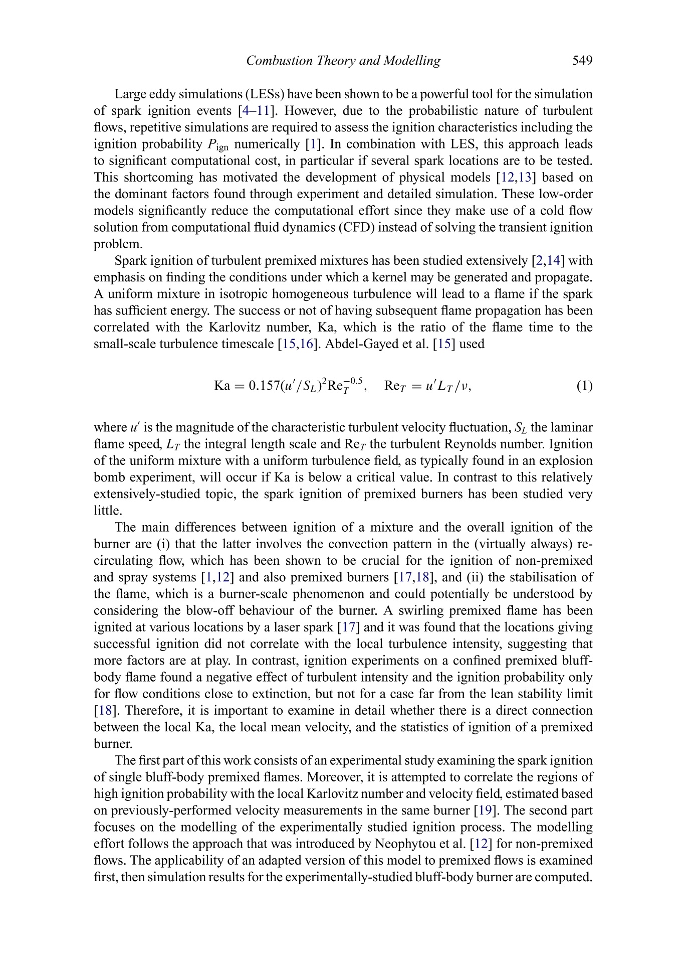
The ignition characteristics of a premixed bluff-body burner under lean conditions were
investigated experimentally and numerically with a physical model focusing on ignition
probability. Visualisation of the flame with a 5 kHz OH* chemiluminescence camera
confirmed that successful ignitions were those associated with the movement of the
kernel upstream, consistent with previous work on non-premixed systems. Performing
many separate ignition trials at the same spark position and flow conditions resulted
in a quantification of the ignition probability Pign, which was found to decrease with
increasing distance downstream of the bluff body and a decrease in equivalence ratio.
Flows corresponding to flames close to the blow-off limit could not be ignited, although
such flames were stable if reached from a richer already ignited condition. A detailed
comparison with the local Karlovitz number and the mean velocity showed that regions
of high Pign are associated with low Ka and negative bulk velocity (i.e. towards the
bluff body), although a direct correlation was not possible. A modelling effort that
takes convection and localised flame quenching into account by tracking stochastic
virtual flame particles, previously validated for non-premixed and spray ignition, was
used to estimate the ignition probability. The applicability of this approach to premixed
flows was first evaluated by investigating the model’s flame propagation mechanism
in a uniform turbulence field, which showed that the model reproduces the bending
behaviour of the ST-versus-u curve. Then ignition simulations of the bluff-body burner
were carried out. The ignition probability map was computed and it was found that the
model reproduces all main trends found in the experimental study.
方案详情

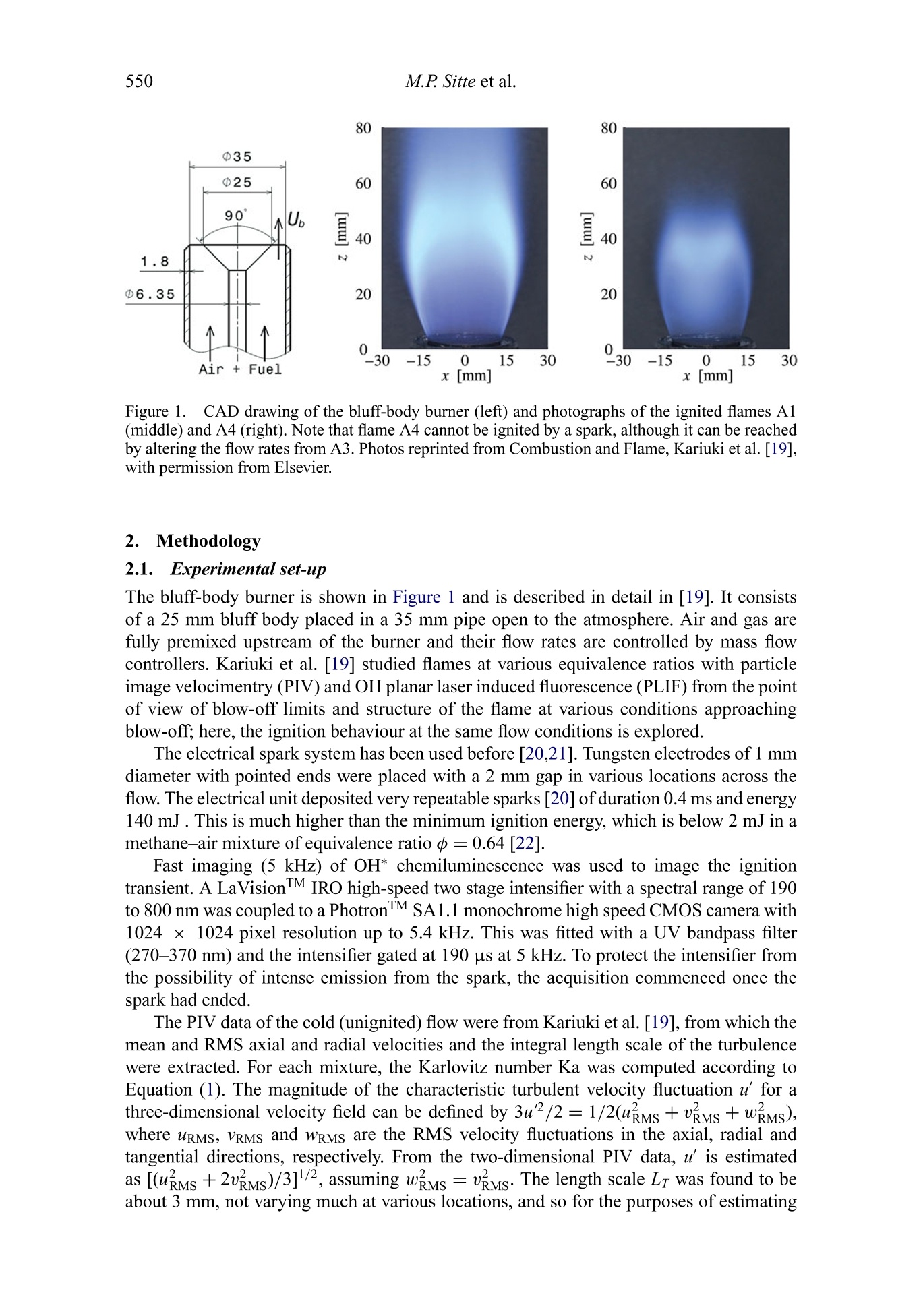
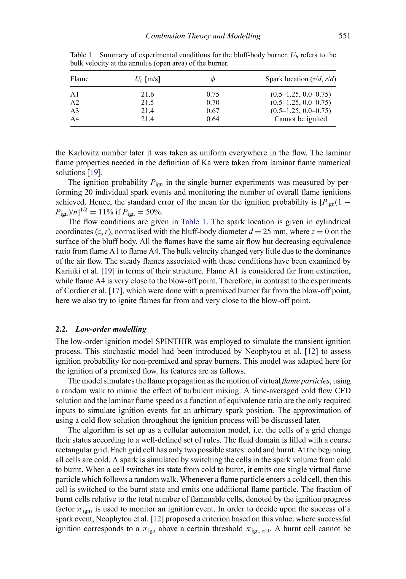
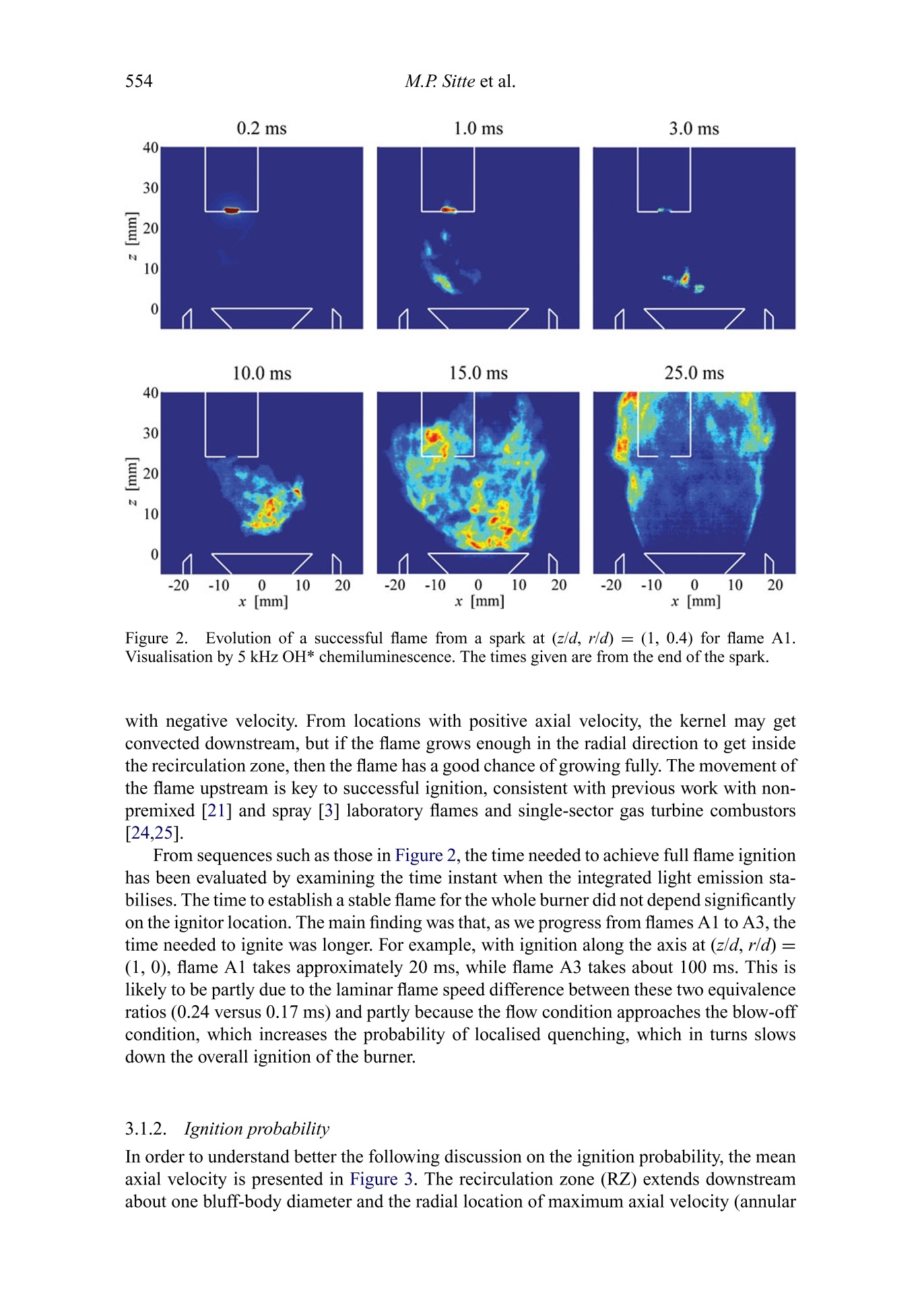
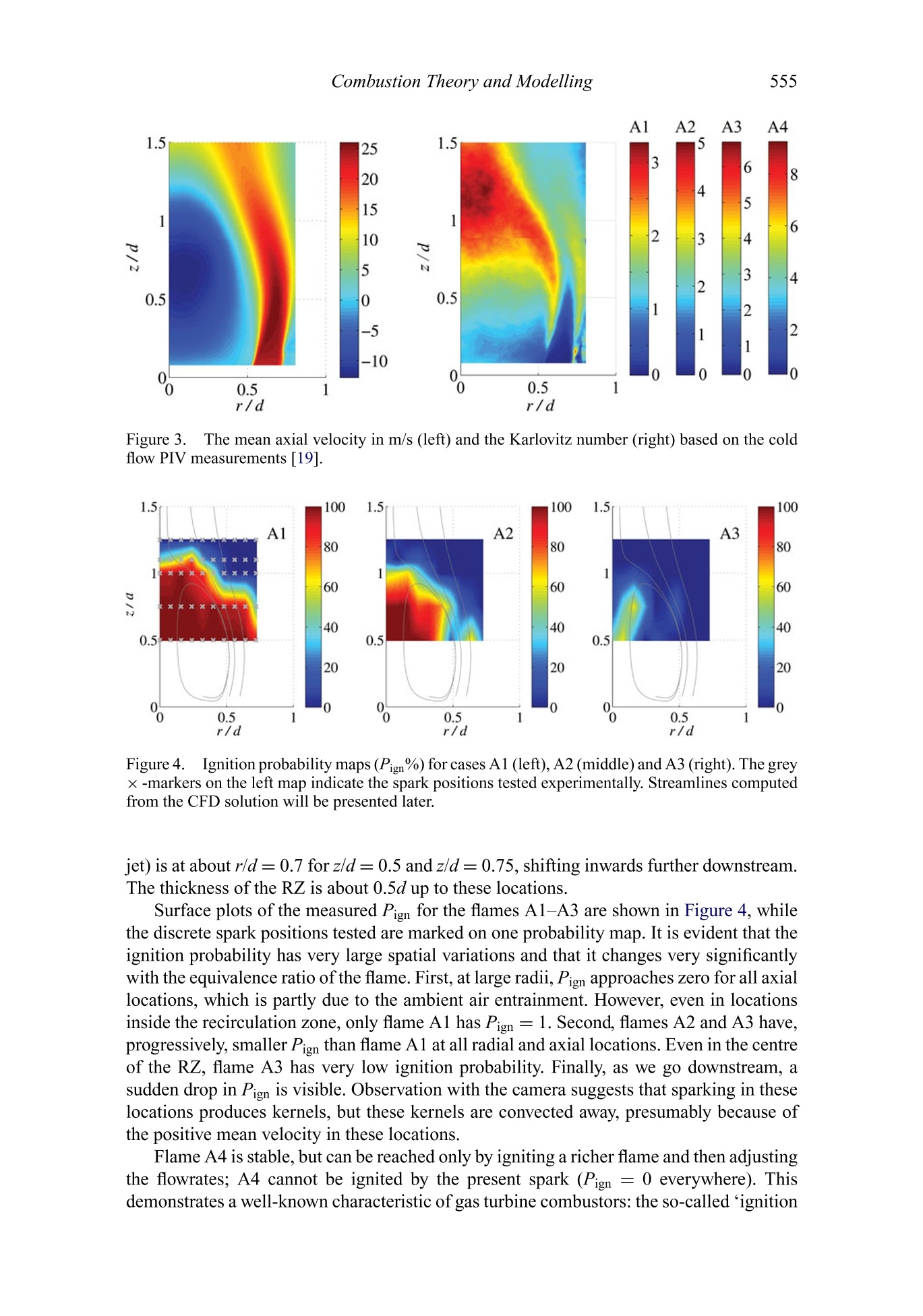
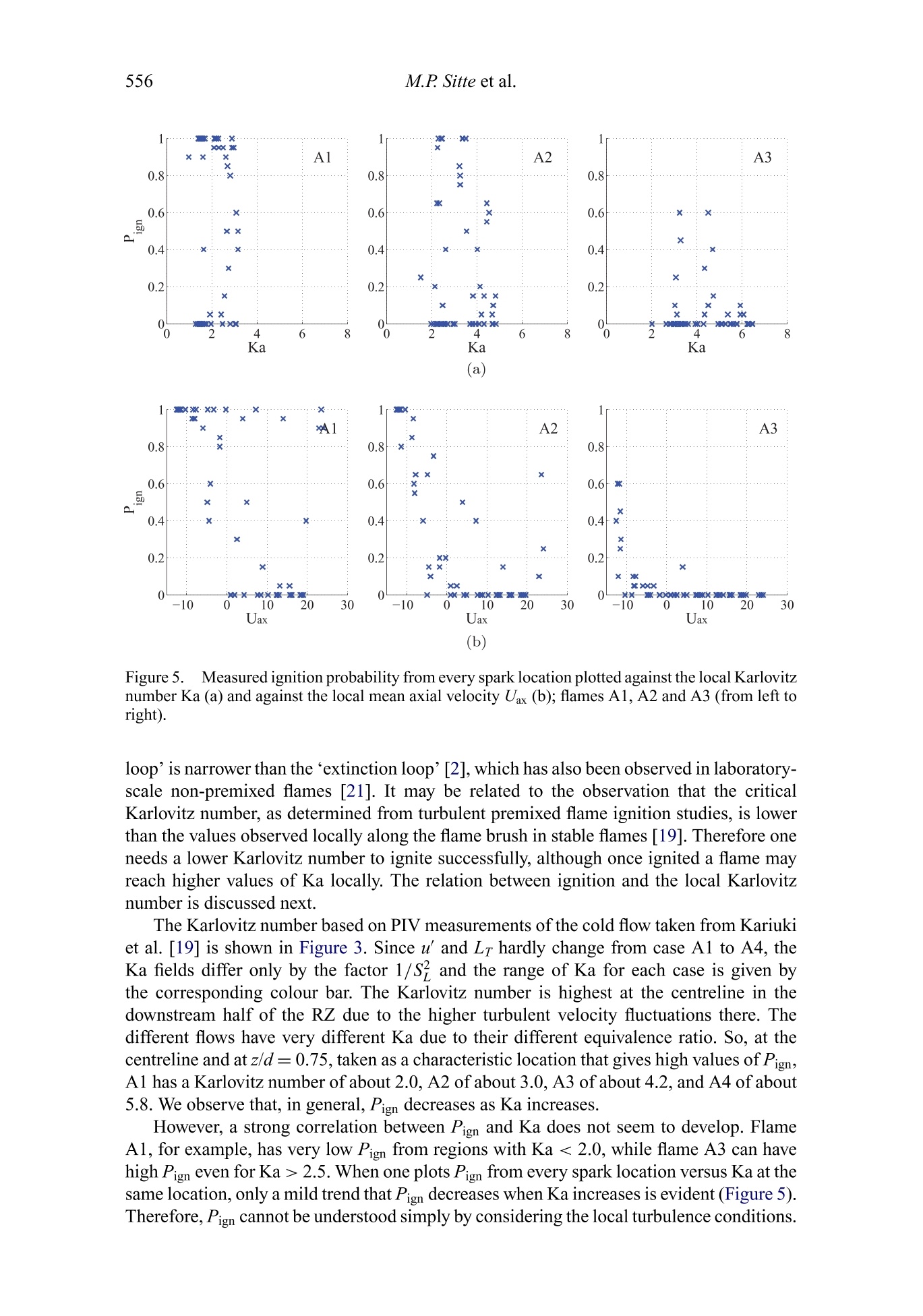
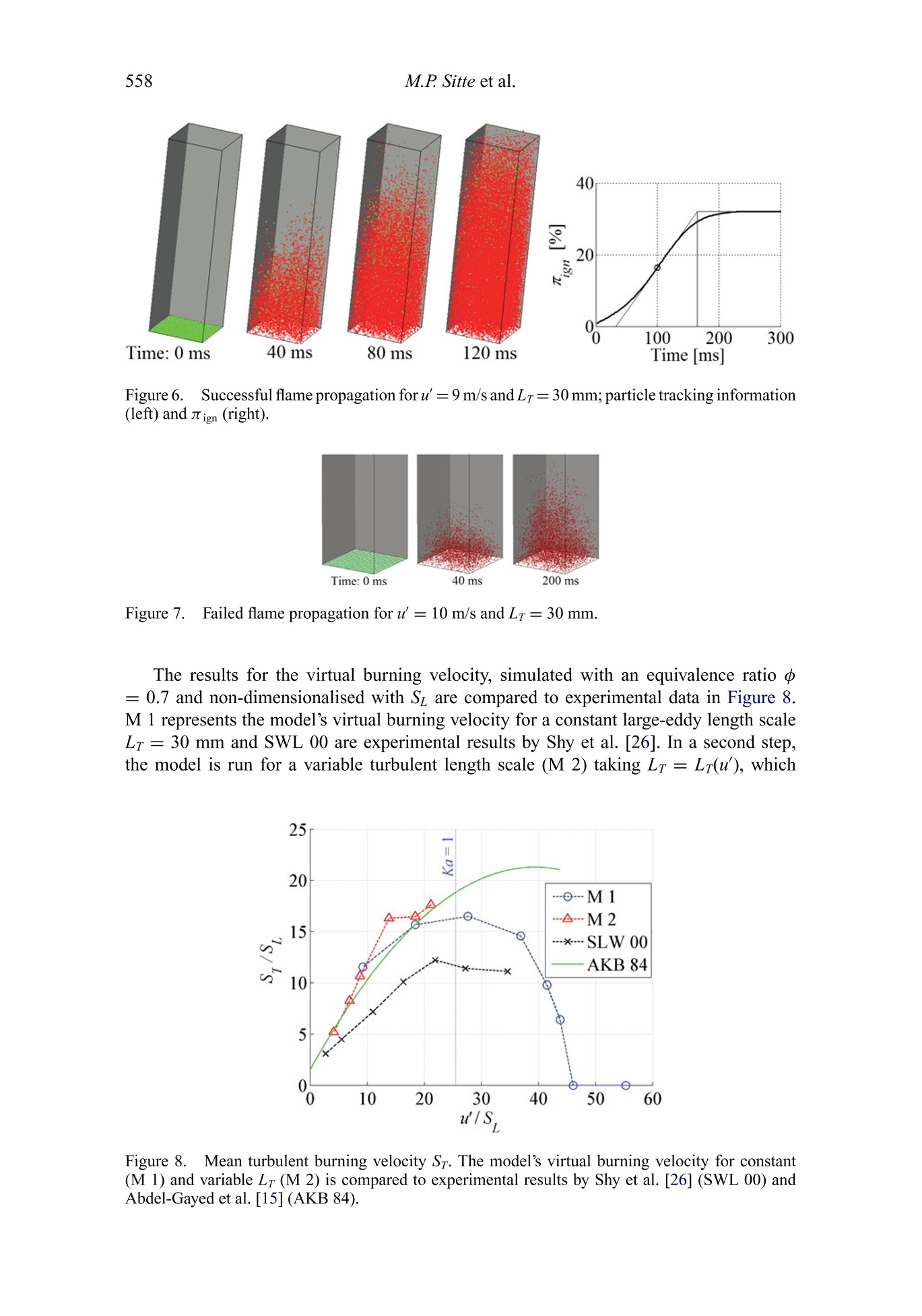
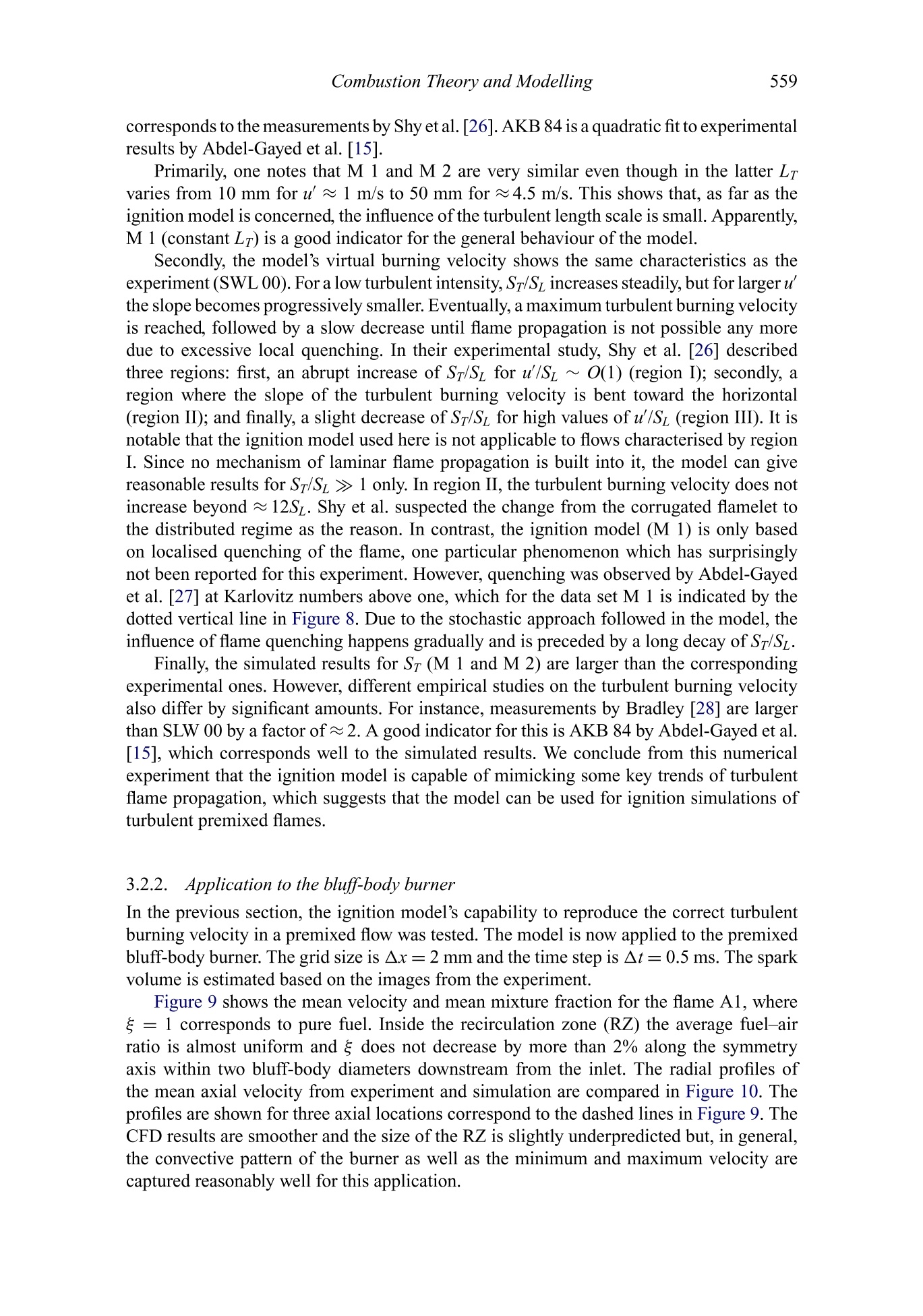
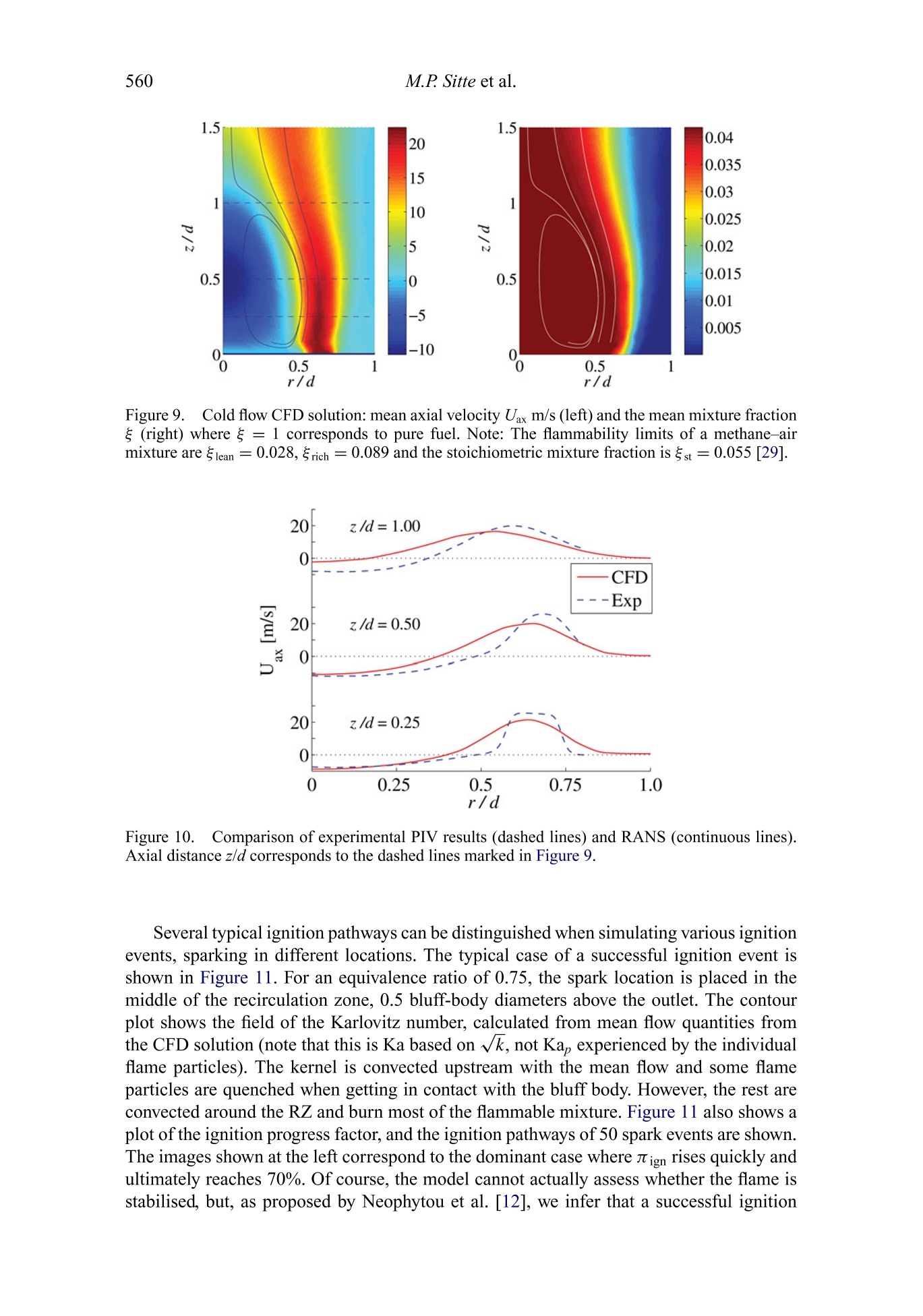
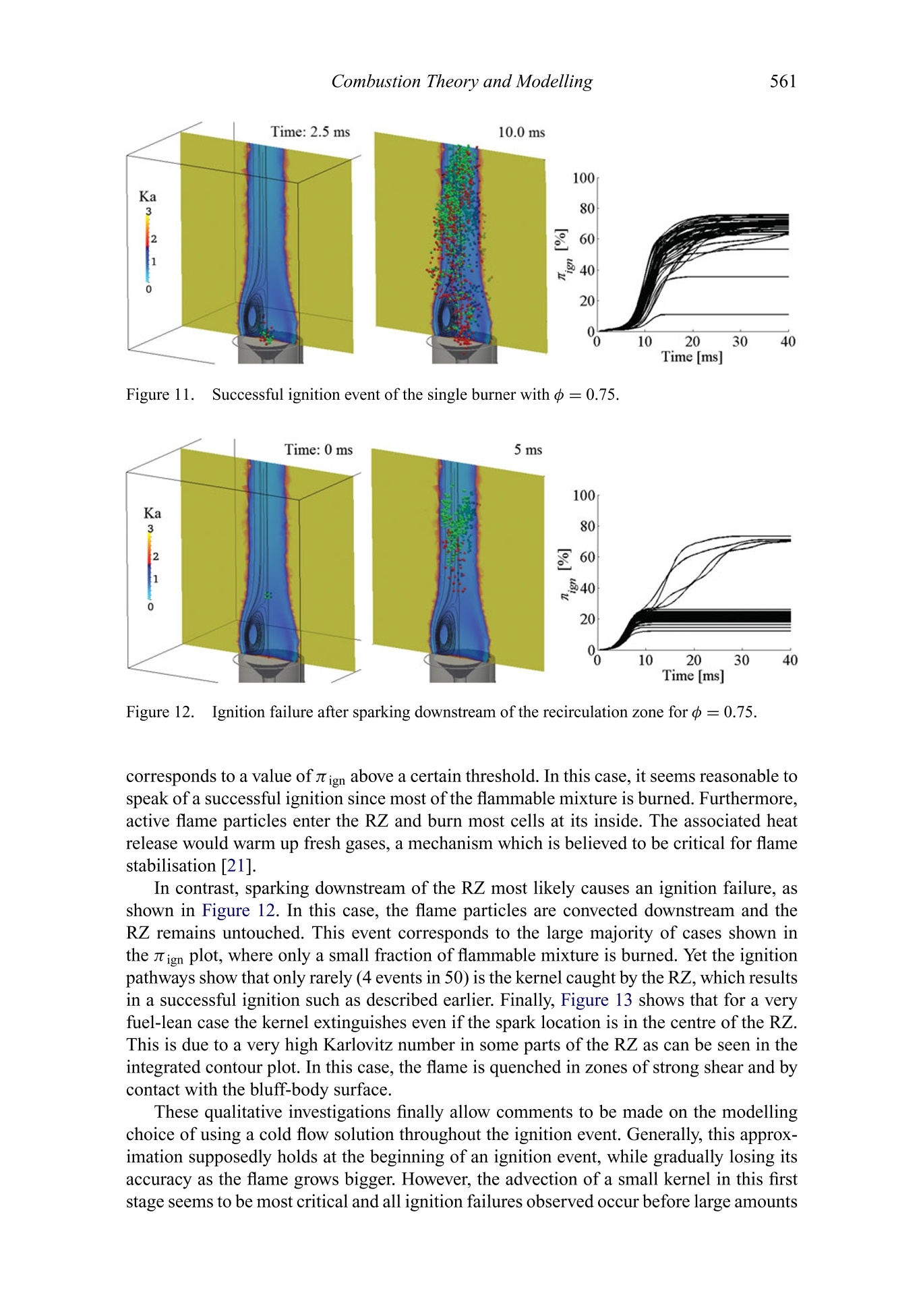
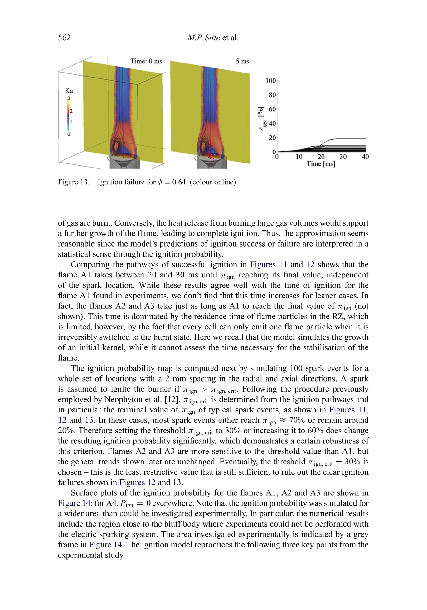
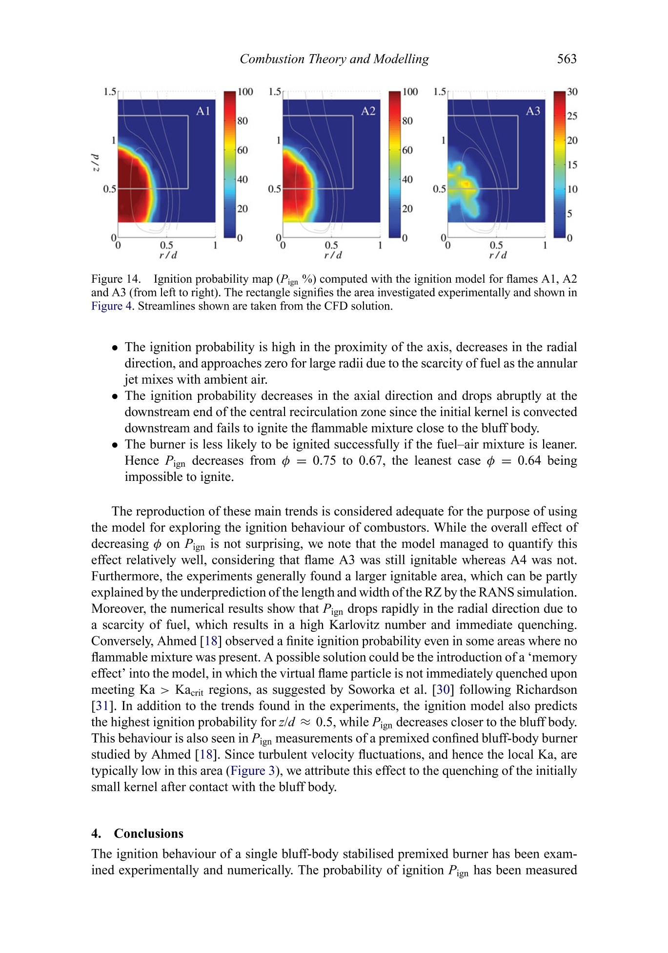
Taylor & FrancisTaylor & Francis GroupCombustion Theory and ModellingISSN: 1364-7830 (Print) 1741-3559 (Online)journal homepage: http://www.tandfonline.com/loi/tctm20 Combustion Theory and Modelling, 2016Taylor & FrancisTaylor &Francis GroupVol. 20,No. 3, 548-565, http://dx.doi.org/10.1080/13647830.2016.1155756 Full Terms & Conditions of access and use can be found atDownload by:[115.171.138.120]Date: 24 August 2016, At: 21:40 Simulations and experiments on the ignitionprobability in turbulent premixed bluff-bodyflames Michael Philip Sitte, Ellen Bach, james Kariuki, Hans-jorg Bauer &Epaminondas Mastorakos To cite this article: Michael Philip Sitte, Ellen Bach, James Kariuki, Hans-jorg Bauer &Epaminondas Mastorakos (2016) Simulations and experiments on the ignition probability inturbulent premixed bluff-body flames, Combustion Theory and Modelling, 20:3, 548-565, DOI:10.1080/13647830.2016.1155756 To link to this article: http://dx.doi.org/10.1080/13647830.2016.1155756 http://www.tandfonline.com/action/journallnformation?journalCode=tctm20 Simulations and experiments on the ignition probability in turbulentpremixed bluff-body flames Michael Philip Sitteeq o a*, Ellen Bach , James Kariuki, Hans-Jorg Bauer andEpaminondas Mastorakos a “Department ofEngineering, University of Cambridge, Cambridge, UK;bInstitut fiir thermische Stromungsmaschinen, Karlsruhe Institute of Technology, Karlsruhe, Germany(Received 15 September 2015; accepted 5 February 2016) The ignition characteristics of a premixed bluff-body burner under lean conditions wereinvestigated experimentally and numerically with a physical model focusing on ignitionprobability. Visualisation of the flame with a 5 kHz OH* chemiluminescence cameraconfirmed that successful ignitions were those associated with the movement of thekernel upstream, consistent with previous work on non-premixed systems. Performingmany separate ignition trials at the same spark position and flow conditions resultedin a quantification of the ignition probability Pign, which was found to decrease withincreasing distance downstream of the bluff body and a decrease in equivalence ratio.Flows corresponding to flames close to the blow-off limit could not be ignited, althoughsuch flames were stable if reached from a richer already ignited condition. A detailedcomparison with the local Karlovitz number and the mean velocity showed that regionsof high Pign are associated with low Ka and negative bulk velocity (i.e. towards thebluff body), although a direct correlation was not possible. A modelling effort thattakes convection and localised flame quenching into account by tracking stochasticvirtual flame particles, previously validated for non-premixed and spray ignition, wasused to estimate the ignition probability. The applicability of this approach to premixedflows was first evaluated by investigating the model’s flame propagation mechanismin a uniform turbulence field, which showed that the model reproduces the bendingbehaviour of the Sp-versus-u’curve.Then ignition simulations of the bluff-body burnerwere carried out. The ignition probability map was computed and it was found that themodel reproduces all main trends found in the experimental study. Keywords: spark ignition; ignition probability; turbulent premixed flames; ignitionmodelling; bluff-body stabilised flames . Introduction Ignition of turbulent flames is very important for a wide range of propulsion applications[1,2]. In recent years, new insights have been developed into the fundamentals of sparkignition processes in non-premixed and spray systems [1,3]. In both experiments andmodelling the key finding is that the kernels from the spark must grow and also be advectedby the flow towards the anchoring points of the flame for the overall burner ignition to besuccessful. Therefore, apart from local processes that affect the success or not of the sparkto develop a kernel, the long-term fate of the flame depends also on the convective patternand on whether the flame may quench later, in other parts of the burner, as it propagates. ( *Corresponding author. Email: mps59@cam.ac.uk ) ( C 2016 The Author(s). Published by In f orma UK Limited, trading as Tay l or & Francis Group ) ( Thi s i s a n O p en A c c ess article d istribute d unde r th e terms of the Creativ e C o C m o m m o m n o s n s A t A tr tt ibution L icense (http://creativecommons.org/licenses/by/4.0/), which permits unrestricted use, dist r ibution, and repr o duction in any medium,provided the original w o rk is properly cited. ) Large eddy simulations (LESs) have been shown to be a powerful tool for the simulationof spark ignition events [4-11]. However, due to the probabilistic nature of turbulentflows, repetitive simulations are required to assess the ignition characteristics including theignition probability Pign numerically [1]. In combination with LES, this approach leadsto significant computational cost, in particular if several spark locations are to be tested.This shortcoming has motivated the development of physical models [12,13] based onthe dominant factors found through experiment and detailed simulation. These low-ordermodels significantly reduce the computational effort since they make use of a cold flowsolution from computational fluid dynamics (CFD) instead of solving the transient ignitionproblem. Spark ignition of turbulent premixed mixtures has been studied extensively [2,14] withemphasis on finding the conditions under which a kernel may be generated and propagate.A uniform mixture in isotropic homogeneous turbulence will lead to a flame if the sparkhas sufficient energy. The success or not of having subsequent flame propagation has beencorrelated with the Karlovitz number, Ka, which is the ratio of the flame time to thesmall-scale turbulence timescale [15,16]. Abdel-Gayed et al. [15] used where u is the magnitude of the characteristic turbulent velocity fluctuation, S, the laminarflame speed, Lr the integral length scale and Rer the turbulent Reynolds number. Ignitionof the uniform mixture with a uniform turbulence field, as typically found in an explosionbomb experiment, will occur if Ka is below a critical value. In contrast to this relativelyextensively-studied topic, the spark ignition of premixed burners has been studied verylittle. The main differences between ignition of a mixture and the overall ignition of theburner are (i) that the latter involves the convection pattern in the (virtually always) re-circulating flow, which has been shown to be crucial for the ignition of non-premixedand spray systems [1,12] and also premixed burners [17,18], and (ii) the stabilisation ofthe flame, which is a burner-scale phenomenon and could potentially be understood byconsidering the blow-off behaviour of the burner. A swirling premixed flame has beenignited at various locations by a laser spark [17] and it was found that the locations givingsuccessful ignition did not correlate with the local turbulence intensity, suggesting thatmore factors are at play. In contrast, ignition experiments on a confined premixed bluff-body flame found a negative effect of turbulent intensity and the ignition probability onlyfor flow conditions close to extinction, but not for a case far from the lean stability limit[18]. Therefore, it is important to examine in detail whether there is a direct connectionbetween the local Ka, the local mean velocity, and the statistics of ignition of a premixedburner. The first part ofthis work consists of an experimental study examining the spark ignitionof single bluff-body premixed flames. Moreover, it is attempted to correlate the regions ofhigh ignition probability with the local Karlovitz number and velocity field, estimated basedon previously-performed velocity measurements in the same burner [19]. The second partfocuses on the modelling of the experimentally studied ignition process. The modellingeffort follows the approach that was introduced by Neophytou et al. [12] for non-premixedflows. The applicability of an adapted version of this model to premixed flows is examinedfirst, then simulation results for the experimentally-studied bluff-body burner are computed. Figure 1. CAD drawing of the bluff-body burner (left) and photographs of the ignited flames A1(middle) and A4 (right). Note that flame A4 cannot be ignited by a spark, although it can be reachedby altering the flow rates from A3. Photos reprinted from Combustion and Flame, Kariuki et al. [19],with permission from Elsevier. 2. Methodology 2.1..Experimental set-up The bluff-body burner is shown in Figure 1 and is described in detail in [19]. It consistsof a 25 mm bluff body placed in a 35 mm pipe open to the atmosphere. Air and gas arefully premixed upstream of the burner and their flow rates are controlled by mass flowcontrollers. Kariuki et al. [19] studied flames at various equivalence ratios with particleimage velocimentry (PIV) and OH planar laser induced fluorescence (PLIF) from the pointof view of blow-off limits and structure of the flame at various conditions approachingblow-off; here, the ignition behaviour at the same flow conditions is explored. The electrical spark system has been used before [20,21]. Tungsten electrodes of 1 mmdiameter with pointed ends were placed with a 2 mm gap in various locations across theflow. The electrical unit deposited very repeatable sparks [20] of duration 0.4 ms and energy140 mJ. This is much higher than the minimum ignition energy, which is below 2 mJ in amethane-air mixture of equivalence ratio +=0.64[22]. Fast imaging (5kHz) of OH* chemiluminescence was used to image the ignitiontransient. A LaVisionTM IRO high-speed two stage intensifier with a spectral range of 190to 800 nm was coupled to a PhotronM SA1.1 monochrome high speed CMOS camera with1024 × 1024 pixel resolution up to 5.4 kHz. This was fitted with a UV bandpass filter(270-370 nm) and the intensifier gated at 190 us at 5 kHz. To protect the intensifier fromthe possibility of intense emission from the spark, the acquisition commenced once thespark had ended. The PIV data of the cold (unignited) flow were from Kariuki et al. [19],from which themean and RMS axial and radial velocities and the integral length scale of the turbulencewere extracted. For each mixture, the Karlovitz number Ka was computed according toEquation (1). The magnitude of the characteristic turbulent velocity fluctuation u for athree-dimensional velocity field can be defined by 3u"/2=1/2(uRMs+vRMs+wpMs),where URMS, VRMs and wRMs are the RMS velocity fluctuations in the axial, radial andtangential directions, respectively. From the two-dimensional PIV data, u’ is estimatedas [(RMs +2vRMs)/3]1/2, assuming wRMs =veMs. The length scale Lr was found to beabout 3 mm, not varying much at various locations, and so for the purposes of estimating Table 11SSummary of experimental conditions for the bluff-body burner. U, refers to thebulk velocity at the annulus (open area) of the burner. Flame U[m/s] 中 Spark location (z/d,rld) A1 21.6 0.75 (0.5-1.25,0.0-0.75) A2 21.5 0.70 (0.5-1.25,0.0-0.75) A3 21.4 0.67 (0.5-1.25,0.0-0.75) A4 21.4 0.64 Cannot be ignited the Karlovitz number later it was taken as uniform everywhere in the flow. The laminarflame properties needed in the definition of Ka were taken from laminar flame numericalsolutions [19]. The ignition probability Pign in the single-burner experiments was measured by per-forming 20 individual spark events and monitoring the number of overall flame ignitionsachieved. Hence, the standard error of the mean for the ignition probability is [Pign(1-Pign)/n]1/2=11% if Pign=50%. The flow conditions are given in Table 1. The spark location is given in cylindricalcoordinates (z, r), normalised with the bluff-body diameter d=25 mm, where z=0 on thesurface of the bluff body.All the flames have the same air flow but decreasing equivalenceratio from flame A1 to flame A4. The bulk velocity changed very little due to the dominanceof the air flow. The steady flames associated with these conditions have been examined byKariuki et al. [19] in terms of their structure. Flame A1 is considered far from extinction,while flame A4 is very close to the blow-off point. Therefore, in contrast to the experimentsof Cordier et al. [17], which were done with a premixed burner far from the blow-off point,here we also try to ignite flames far from and very close to the blow-off point. 2.2.Low-order modelling The low-order ignition model SPINTHIR was employed to simulate the transient ignitionprocess. This stochastic model had been introduced by Neophytou et al. [12] to assessignition probability for non-premixed and spray burners. This model was adapted here forthe ignition of a premixed flow. Its features are as follows. The model simulates the flame propagation as the motion of virtualflame particles, usinga random walk to mimic the effect of turbulent mixing. A time-averaged cold flow CFDsolution and the laminar flame speed as a function ofequivalence ratio are the only requiredinputs to simulate ignition events for an arbitrary spark position. The approximation ofusing a cold flow solution throughout the ignition process will be discussed later. The algorithm is set up as a cellular automaton model, i.e. the cells of a grid changetheir status according to a well-defined set of rules. The fluid domain is filled with a coarserectangular grid. Each grid cell has only two possible states: cold and burnt. At the beginningall cells are cold. A spark is simulated by switching the cells in the spark volume from coldto burnt. When a cell switches its state from cold to burnt, it emits one single virtual flameparticle which follows a random walk. Whenever a flame particle enters a cold cell, then thiscell is switched to the burnt state and emits one additional flame particle. The fraction ofburnt cells relative to the total number of flammable cells, denoted by the ignition progressfactor Jign, is used to monitor an ignition event. In order to decide upon the success of aspark event, Neophytou et al. [12] proposed a criterion based on this value, where successfulignition corresponds to a Jign above a certain threshold ign,crit. A burnt cell cannot be switched back to its original cold state. This choice makes nign an unambiguous metricfor the burner volume that has been visited by the cloud of flame particles. While thisirreversibility caps the maximum number of particles in one simulation, it is without anyfurther consequences on the evolution of the particle cloud, since the particles once emitteddo not interact with the cells any more (see below). As such the cells’state constitutes anabstract measure of the ignition progress, which does not coincide with the position of theflame. The ignition process is driven by the virtual flame particles. These particles are emittedby the cells and follow a random walk until being quenched by strong turbulence. Hence,the random walk mimics the motion of a small kernel in the turbulent flow field. Moreover,the cloud of particles grows as additional ones are emitted by the cells. In Section 3.2.1,the evolution of the particle cloud is investigated in terms of its capability to reproducefeatures of flame growth and propagation. The random walk is given by a simplified Langevin model described by Equations (2)and (3), where Ax, denotes the displacement vector of a particle p during the time intervalAt and its respective velocity is U,. Co =2 is a constant and N, a vector with a randomdirection whose length follows a Gaussian distribution N(0,1). The other parameters aretaken from the cold flow CFD solution.Here, Lr is the integral length scale and u’ theturbulent velocity fluctuation estimated as √k, where k is the turbulent kinetic energy; ǔ isthe local Favre averaged velocity and e the local turbulent dissipation rate. Note that thismodel does not consider the effects of molecular diffusion or gas expansion. Additionally, an extinction criterion is applied to decide whether a flame particle remainsactive or extinguishes. This flame quenching criterion is based on the Karlovitz numberas introduced by Abdel-Gayed and Bradley [23]. For each flame particle the Karlovitznumber is calculated in every time step according to Equation (1). In the original modelfor a non-premixed flow [12] Lr, u’~√k are taken from the cold flow CFD solution andan equation is solved for the mixture fraction of a flame particle 5p, which is required forthe computation of SL(5p). The flame particle extinguishes ifKa, exceeds the critical valueKacrit =1.5. This model was adapted for premixed burners and two modifications were introduced,the most important being a randomisation of the Karlovitz number. In the original model[12], a locally constant value u'(x) from the cold flow CFD solution was used to computeKa,. Of course, in the non-premixed case, the availability of fuel most prominently deter-mines the survival of a kernel and the probabilistic nature of local flame quenching wasdue to random fluctuations of the mixture fraction. On the other hand, in a premixed flowthis means that all flame particles passing through the same flow region experience thesame u resulting in the same Ka,. Instead of using the locally constant u from CFD inthe present premixed case, the Karlovitz criterion now uses the turbulent fluctuation thatthe particle is actually experiencing through the random walk. In other words, theparticle’sKarlovitz number is higher if its motion is characterised by strong velocity fluctuations.Hence, the parts of the flame exposed to violent turbulence are more likely to extinguish.The second modification of the model is an extension to account for the case of flame-wall contact. Considering initially cold walls of the combustion chamber, all flame particles areextinguished if they enter into contact with a wall. Hence the position of all active flameparticles is tested after every step of the random walk. Those particles that are suddenlyfound outside the domain have either left through an open surface with an outlet boundarycondition or a wall. In the latter case they are considered to be quenched by wall contactand are, thus, switched to the extinguished state. Neophytou et al. [12] proposed guidelines for the time step and the grid size. Thesesuggestions are based on necessity to assure consistency with the random walk and theKarlovitz criterion from a statistical point of view. Consequently, the time step ▲t< Lpluand the grid spacing 18nk < ▲x≤2(Coe▲t)1/2At, where n is the Kolmogorov scale,can be retained when the model is used for premixed flows. The spatial discretisation isdiscussed thoroughly in the appendix of[12], concluding that grid dependence is small ifthe above-mentioned limits are respected. 2.3.. Cold flow CFD solution The cold flow field was computed with a steady-state Reynolds-averaged Navier-Stokes(RANS) simulation using the commercial CFD software ANSYS Fluent@. The turbulencemodel used was a realisable k-s model with standard parameters. The computational domainhad a cylindrical shape of diameter 200 mm and height 200 mm with an inflow boundarycondition at the level of the annulus between bluff body and pipe. The velocity and turbulentintensity at the inlet were fixed according to experimental data [19].Moreover, the mixturefraction at the inlet was fixed at the value;=中/(中+[1 -5st]/5st), corresponding to thethe equivalence ratio o indicated in Table 1, while 5st=0.055 is the stoichiometric mixturefraction. Zero-gradient boundary conditions for the velocity and the mixture fraction aswell as constant pressure were set at the outlet surface. A far-field condition was appliedat the boundaries to the ambient air at the bottom and the sides of the domain with zerogradient velocity and pressure as well as fixed mixture fraction 5=0. The surface of thebluff body was modelled as a wall with a no-slip boundary condition. The domain wasmeshed with an unstructured tetrahedral grid with 130k nodes. The grid was refined in theregion of the recirculation zone and around the inlet, where the grid size was 1.5 mm. For the use ofthe cold flow field by the ignition model, the CFD solution was interpolatedon a regular grid (grid spacing 2 mm) in a cubic domain with an edge length of 100 mm.The edges of this domain are indicated in Figures 11, 12 and 13. 3. Results and discussion 3.1.. Experiments 3.1.1.IIgnition visualisation Photographs of the ignited premixed flame at conditions A1 and A4 are shown in Figure 1.Flame A4 is very close to the blow-off point (at this velocity, blow off occurs at anequivalence ratio 0.63), while flames A3 to A1 are progressively farther from the blow-offcondition. A sequence of a successful ignition event for flame A1 from spark position (z/d, rld)=(1,0.4) is shown in Figure 2. It is evident that the kernel has moved off the spark inthe upstream direction and eventually grows to ignite the full flame. At times during theflame evolution, the flamelet may be small, but even a small flame surviving upstreamwill be enough to ignite the burner. Similar evolutions are observed from other locations 0.2 ms 1.0 ms 3.0 ms 40 30 20 10 O 10.0 ms 15.0 ms 25.0 ms 40 30 20 10 Figure 2. Evolution of a successful flame from a spark at (z/d, r/d)= (1, 0.4) for flame A1.Visualisation by 5 kHz OH* chemiluminescence. The times given are from the end of the spark. with negative velocity. From locations with positive axial velocity, the kernel may getconvected downstream, but if the flame grows enough in the radial direction to get insidethe recirculation zone, then the flame has a good chance of growing fully. The movement ofthe flame upstream is key to successful ignition, consistent with previous work with non-premixed [21] and spray [3] laboratory flames and single-sector gas turbine combustors[24,25]. From sequences such as those in Figure 2, the time needed to achieve full flame ignitionhas been evaluated by examining the time instant when the integrated light emission sta-bilises. The time to establish a stable flame for the whole burner did not depend significantlyon the ignitor location. The main finding was that, as we progress from flames A1 to A3, thetime needed to ignite was longer. For example, with ignition along the axis at (z/d,rld)=(1, 0), flame Al takes approximately 20 ms, while flame A3 takes about 100 ms. This islikely to be partly due to the laminar flame speed difference between these two equivalenceratios (0.24 versus 0.17 ms) and partly because the flow condition approaches the blow-offcondition, which increases the probability of localised quenching, which in turns slowsdown the overall ignition of the burner. 3.1.22..I1gnition probability In order to understand better the following discussion on the ignition probability, the meanaxial velocity is presented in Figure 3. The recirculation zone (RZ) extends downstreamabout one bluff-body diameter and the radial location of maximum axial velocity (annular A1 A2 A3 A4 Figure 3. The mean axial velocity in m/s (left) and the Karlovitz number (right) based on the coldflow PIV measurements [191. Figure 4.Ignition probability maps (Pign%) for cases A1 (left), A2 (middle)and A3 (right). The greyx-markers on the left map indicate the spark positions tested experimentally. Streamlines computedfrom the CFD solution will be presented later. jet) is at about r/d=0.7 for z/d=0.5 and z/d=0.75, shifting inwards further downstream.The thickness of the RZ is about 0.5d up to these locations. Surface plots of the measured Pign for the flames A1-A3 are shown in Figure 4, whilethe discrete spark positions tested are marked on one probability map. It is evident that theignition probability has very large spatial variations and that it changes very significantlywith the equivalence ratio of the flame. First, at large radii, Pign approaches zero for all axiallocations, which is partly due to the ambient air entrainment. However, even in locationsinside the recirculation zone, only flame A1 has Pign=1. Second, flames A2 and A3 have,progressively,smaller Pign than flame A1 at all radial and axial locations. Even in the centreof the RZ, flame A3 has very low ignition probability. Finally, as we go downstream, asudden drop in Pign is visible. Observation with the camera suggests that sparking in theselocations produces kernels, but these kernels are convected away, presumably because ofthe positive mean velocity in these locations. Flame A4 is stable, but can be reached only by igniting a richer flame and then adjustingthe flowrates; A4 cannot be ignited by the present spark (Pign =0 everywhere). Thisdemonstrates a well-known characteristic of gas turbine combustors: the so-called ‘ignition Figure 5..Measuredignition probability from every spark location plotted against the local Karlovitznumber Ka (a) and against the local mean axial velocity Uax (b); flames A1, A2 and A3 (from left toright). loop’is narrower than the ‘extinction loop’[2],which has also been observed in laboratory-scale non-premixed flames [21]. It may be related to the observation that the criticalKarlovitz number, as determined from turbulent premixed flame ignition studies, is lowerthan the values observed locally along the flame brush in stable flames [19]. Therefore oneneeds a lower Karlovitz number to ignite successfully, although once ignited a flame mayreach higher values of Ka locally. The relation between ignition and the local Karlovitznumber is discussed next. The Karlovitz number based on PIV measurements of the cold flow taken from Kariukiet al. [19]is shown in Figure 3. Since u and Lr hardly change from case A1 to A4, theKa fields differ only by the factor 1/S and the range of Ka for each case is given by'Lthe corresponding colour bar. The Karlovitz number is highest at the centreline in thedownstream half of the RZ due to the higher turbulent velocity fluctuations there. Thedifferent flows have very different Ka due to their different equivalence ratio. So, at thecentreline and at z/d= 0.75, taken as a characteristic location that gives high values of Pign,A1 has a Karlovitz number of about 2.0, A2 of about 3.0, A3 of about 4.2, and A4 of about5.8. We observe that, in general, Pign decreases as Ka increases. However, a strong correlation between Pign and Ka does not seem to develop. FlameA1, for example, has very low Pign from regions with Ka < 2.0, while flame A3 can havehigh Pign even for Ka> 2.5. When one plots Pign from every spark location versus Ka at thesame location, only a mild trend that Pign decreases when Ka increases is evident (Figure 5).Therefore, Pign cannot be understood simply by considering the local turbulence conditions. When one plots the Pign from every spark location versus the mean axial velocity at thesame location, a trend that Pign increases when the velocity is negative becomes evident(Figure 5). Only flame A1 (the richest one examined here) can be ignited with high Pign insome regions with positive axial velocity. It is clear therefore that successful ignition events arise, in a statistical sense, from flowconditions and spark locations that not only have low Ka, but also negative axial velocity,so that the kernels not only survive unquenched, but are also convected towards the bluffbody. This is in perfect agreement with the discussion and review of experimental datafrom non-premixed and spray burners in Neophytou et al.[12]. The present data emphasisefurther the effect of mean convection and local turbulence on the ignition of burners. Theyalso suggest that to be able to capture ignition transients properly with LES, the combustionmodel must include local quenching. This seems to be included in some efforts [6-8], butfurther validation is necessary and the present data can be used for that purpose. 3.2.Ignition modelling 3.2.1. Plrediction ofthe turbulent burning velocity Experimental findings showed that local flow quantities may not be sufficient to judge theignitability of a burner and underlined the importance of convection of the initial kernelalso being exposed to localised extinction. These key features are included in a simplifiedphysical model that was proposed by Neophytou et al. [12] for the ignition of non-premixedflows. Whereas this model was successfully applied to the ignition of non-premixed andspray flames, the approach has not yet been used to simulate the ignition of a premixedflame. To assess the applicability of the model to premixed flows, its flame propagationmechanism is investigated. The turbulent burning velocity Sr is chosen as the key quantityto judge the quality of this feature and the following test is performed. The ignition model’svirtual burning velocity is defined over the time the flame particles take to cross a givendistance. In order to determine this quantity, the model is used on an elongated domainwith square cross section, filled with a uniform air-fuel mixture. In the absence of a meanflow, the velocity field is given by non-decaying, uniform, isotropic turbulence. The domainis at least 2Lr wide and 10Lr long to limit boundary effects. In addition, the flame-wallinteraction is changed and incoming flame particles are now reflected to cancel out effectsof limited size. For the range of velocity fluctuations investigated, the grid size is set toAx=2 mm and the time step is 2 ms for u’<10 m/s and 1 ms above. Figure 6 shows a typical case offlame propagation after having initiated the ignition byswitching all cells on one surface to the burnt state. Att=0 ms all flame particles are active;at later times the majority is extinguished, with a few active ones driving the propagtion. Inorder to monitor the flame propagation, the ignition progress factor 7 ign - the fraction ofburnt cells in the domain evolving in time- is a useful indicator. It corresponds closely tothe spatial expansion of the particle cloud but is more clearly defined. The graph is smoothand rises almost linearly for 70 1 only. In region II, the turbulent burning velocity does notincrease beyond≈12Sz. Shy et al. suspected the change from the corrugated flamelet tothe distributed regime as the reason. In contrast, the ignition model (M 1) is only basedon localised quenching of the flame, one particular phenomenon which has surprisinglynot been reported for this experiment. However, quenching was observed by Abdel-Gayedet al. [27] at Karlovitz numbers above one, which for the data set M 1 is indicated by thedotted vertical line in Figure 8. Due to the stochastic approach followed in the model, theinfluence of flame quenching happens gradually and is preceded by a long decay of Sy/SL. Finally, the simulated results for Sr (M 1 and M 2) are larger than the correspondingexperimental ones. However, different empirical studies on the turbulent burning velocityalso differ by significant amounts. For instance, measurements by Bradley [28] are largerthan SLW 00 by a factor of~2. A good indicator for this is AKB 84 by Abdel-Gayed et al.[15], which corresponds well to the simulated results. We conclude from this numericalexperiment that the ignition model is capable of mimicking some key trends of turbulentflame propagation, which suggests that the model can be used for ignition simulations ofturbulent premixed flames. 3.2.2..A1pplication to the bluff-body burner In the previous section, the ignition model's capability to reproduce the correct turbulentburning velocity in a premixed flow was tested. The model is now applied to the premixedbluff-body burner. The grid size is △x=2 mm and the time step is t=0.5 ms. The sparkvolume is estimated based on the images from the experiment. Figure 9 shows the mean velocity and mean mixture fraction for the flame A1, where=1 corresponds to pure fuel. Inside the recirculation zone (RZ) the average fuel-airratio is almost uniform and does not decrease by more than 2% along the symmetryaxis within two bluff-body diameters downstream from the inlet. The radial profiles ofthe mean axial velocity from experiment and simulation are compared in Figure 10. Theprofiles are shown for three axial locations correspond to the dashed lines in Figure 9. TheCFD results are smoother and the size of the RZ is slightly underpredicted but, in general,the convective pattern of the burner as well as the minimum and maximum velocity arecaptured reasonably well for this application. Figure9.. Cold flow CFD solution: mean axial velocity Uax m/s (left) and the mean mixture fraction (right) where =1 corresponds to pure fuel. Note: The flammability limits of a methane-airmixture arelean =0.028,5rich =0.089 and the stoichiometric mixture fraction is 5st =0.055 [29]. Figure 10.. Comparison of experimental PIV results (dashed lines) and RANS (continuous lines).Axial distance z/d corresponds to the dashed lines marked in Figure 9. Several typical ignition pathways can be distinguished when simulating various ignitionevents, sparking in different locations. The typical case of a successful ignition event isshown in Figure 11. For an equivalence ratio of 0.75, the spark location is placed in themiddle of the recirculation zone, 0.5 bluff-body diameters above the outlet. The contourplot shows the field of the Karlovitz number, calculated from mean flow quantities fromthe CFD solution (note that this is Ka based on √k, not Ka, experienced by the individualflame particles). The kernel is convected upstream with the mean flow and some flameparticles are quenched when getting in contact with the bluff body. However, the rest areconvected around the RZ and burn most of the flammable mixture. Figure 11 also shows aplot of the ignition progress factor, and the ignition pathways of 50 spark events are shown.The images shown at the left correspond to the dominant case where ign rises quickly andultimately reaches 70%.Of course, the model cannot actually assess whether the flame isstabilised, but, as proposed by Neophytou et al. [12], we infer that a successful ignition Figure 11.. Successful ignition event of the single burner with =0.75. Figure 12.Ignition failure after sparking downstream of the recirculation zone for 中=0.75 corresponds to a value of Jign above a certain threshold. In this case, it seems reasonable tospeak of a successful ignition since most of the flammable mixture is burned. Furthermore,active flame particles enter the RZ and burn most cells at its inside. The associated heatrelease would warm up fresh gases, a mechanism which is believed to be critical for flamestabilisation [21]. In contrast, sparking downstream of the RZ most likely causes an ignition failure, asshown in Figure 12. In this case, the flame particles are convected downstream and theRZ remains untouched. This event corresponds to the large majority of cases shown inthe T ign plot, where only a small fraction of flammable mixture is burned. Yet the ignitionpathways show that only rarely (4 events in 50) is the kernel caught by the RZ, which resultsin a successful ignition such as described earlier. Finally, Figure 13 shows that for a veryfuel-lean case the kernel extinguishes even if the spark location is in the centre of the RZ.This is due to a very high Karlovitz number in some parts of the RZ as can be seen in theintegrated contour plot. In this case, the flame is quenched in zones of strong shear and bycontact with the bluff-body surface. These qualitative investigations finally allow comments to be made on the modellingchoice of using a cold flow solution throughout the ignition event. Generally, this approx-imation supposedly holds at the beginning of an ignition event, while gradually losing itsaccuracy as the flame grows bigger. However, the advection of a small kernel in this firststage seems to be most critical and all ignition failures observed occur before large amounts Figure 13.Ignition failure for 中=0.64. (colour online) of gas are burnt. Conversely, the heat release from burning large gas volumes would supporta further growth of the flame, leading to complete ignition. Thus, the approximation seemsreasonable since the model’s predictions of ignition success or failure are interpreted in astatistical sense through the ignition probability. Comparing the pathways of successful ignition in Figures 11 and 12 shows that theflame A1 takes between 20 and 30 ms until nign reaching its final value, independentof the spark location. While these results agree well with the time of ignition for theflame A1 found in experiments, we don’t find that this time increases for leaner cases. Infact, the flames A2 and A3 take just as long as A1 to reach the final value of n ign (notshown). This time is dominated by the residence time of flame particles in the RZ, whichis limited, however, by the fact that every cell can only emit one flame particle when it isirreversibly switched to the burnt state. Here we recall that the model simulates the growthof an initial kernel, while it cannot assess the time necessary for the stabilisation of theflame. The ignition probability map is computed next by simulating 100 spark events for awhole set of locations with a 2 mm spacing in the radial and axial directions. A sparkis assumed to ignite the burner if nign> Jign,crit. Following the procedure previouslyemployed by Neophytou et al. [12],Jign, crit is determined from the ignition pathways andin particular the terminal value of Jign of typical spark events, as shown in Figures 11,12 and 13. In these cases, most spark events either reach nign ~ 70% or remain around20%.Therefore setting the threshold Jign, crit to 30% or increasing it to 60% does changethe resulting ignition probability significantly, which demonstrates a certain robustness ofthis criterion. Flames A2 and A3 are more sensitive to the threshold value than A1, butthe general trends shown later are unchanged. Eventually, the threshold J ign, crit =30% ischosen- this is the least restrictive value that is still sufficient to rule out the clear ignitionfailures shown in Figures 12 and 13. Surface plots of the ignition probability for the flames A1, A2 and A3 are shown inFigure 14; for A4, Pign =0 everywhere. Note that the ignition probability was simulated fora wider area than could be investigated experimentally. In particular, the numerical resultsinclude the region close to the bluff body where experiments could not be performed withthe electric sparking system. The area investigated experimentally is indicated by a greyframe in Figure 14. The ignition model reproduces the following three key points from theexperimental study. Figure 1.4 .Ignition probability map (Pign %) computed with the ignition model for flames A1, A2and A3 (from left to right). The rectangle signifies the area investigated experimentally and shown inFigure 4. Streamlines shown are taken from the CFD solution. ●The ignition probability is high in the proximity of the axis, decreases in the radialdirection, and approaches zero for large radii due to the scarcity of fuel as the annulariet mixes with ambient air. · The ignition probability decreases in the axial direction and drops abruptly at thedownstream end of the central recirculation zone since the initial kernel is convecteddownstream and fails to ignite the flammable mixture close to the bluff body. The burner is less likely to be ignited successfully if the fuel-air mixture is leaner.Hence Pign decreases from = 0.75 to 0.67, the leanest case =0.64 beingimpossible to ignite. The reproduction of these main trends is considered adequate for the purpose of usingthe model for exploring the ignition behaviour of combustors. While the overall effect ofdecreasing on Pign is not surprising, we note that the model managed to quantify thiseffect relatively well, considering that flame A3 was still ignitable whereas A4 was not.Furthermore, the experiments generally found a larger ignitable area, which can be partlyexplained by the underprediction ofthe length and width ofthe RZ by the RANS simulation.Moreover, the numerical results show that Pign drops rapidly in the radial direction due toa scarcity of fuel, which results in a high Karlovitz number and immediate quenching.Conversely, Ahmed [18] observed a finite ignition probability even in some areas where noflammable mixture was present. A possible solution could be the introduction of a ‘memoryeffect'into the model, in which the virtual flame particle is not immediately quenched uponmeeting Ka >Kacrit regions, as suggested by Soworka et al. [30] following Richardson[31]. In addition to the trends found in the experiments, the ignition model also predictsthe highest ignition probability for z/d 0.5, while Pign decreases closer to the bluff body.This behaviour is also seen in Pign measurements of a premixed confined bluff-body burnerstudied by Ahmed [18]. Since turbulent velocity fluctuations, and hence the local Ka, aretypically low in this area (Figure 3), we attribute this effect to the quenching of the initiallysmall kernel after contact with the bluff body. 4. Conclusions The ignition behaviour of a single bluff-body stabilised premixed burner has been exam-ined experimentally and numerically. The probability of ignition Pign has been measured experimentally at various flow conditions and locations. It was found that sparking insidethe recirculation zone maximised the likelihood of success, although Pign decreased sub-stantially as the flame became leaner. A direct comparison between the local Pign and theestimated Karlovitz number Ka showed that, in general, Pign was high where Ka was low,but an additional condition for high Pign was that the mean velocity had to be negative (i.e.towards the bluff body). The time taken to ignite the flame increased as the equivalenceratio decreased. Flames very close to the blow-off condition could not be ignited by a spark,although they were reachable by igniting a richer flame and adjusting the equivalence ratio. A stochastic low-order ignition model for non-premixed flows has been adapted tothe present premixed case. Simulations on a rectangular domain and in the absence ofmean flow were carried out to assess the models capability of mimicking turbulent flamepropagation. It was found that the model reproduced general trends of the mean turbulentburning velocity as a function of the velocity fluctuation including the ‘bending behaviour’of Sr versus u, suggesting the model's applicability to the ignition process of premixedburners. Indeed, simulation results for the bluff-body burner globally match the findingsfrom the experimental study and, in particular, good agreement is found for the influenceof equivalence ratio and spark location on Pign. Acknowledgements The experiments were carried out by E. Bach, who was a Masters student from Karlsruhe Institute ofTechnology visiting the University of Cambridge in 2011. Disclosure statement No potential conflict of interest was reported by the authors. Funding M.P. Sitte gratefully acknowledges financial support from the Gates Cambridge Trust. ORCID Michael Philip Sitte Dhttp://orcid.org/0000-0002-7502-9858Epaminondas Mastorakos D http://orcid.org/0000-0001-8245-5188 References [1] E. Mastorakos, Ignition of turbulent non-premixed flames, Prog. Energy Combust. Sci. 35(2009), pp. 57-97. A.H. Lefebvre, Gas Turbine Combustion, 2nd ed., Taylor & Francis, London, 1999. T.Marchione, S.F. Ahmed, and E. Mastorakos, Ignition ofturbulent swirling n-heptane sprayflames using single and multiple sparks, Combust. Flame 156 (2009), pp. 166-180. [4]1M. Boileau, G. Staffelbach, B. Cuenot, T.Poinsot, and C. Berat, LES of an ignition sequencein a gas turbine engine, Combust. Flame 154 (2008), pp.2-22. [5]G. Lacaze, E. Richardson, and T. Poinsot, Large eddy simulation of spark ignition in a turbulentmethane jet, Combust. Flame 156 (2009), pp. 1993-2009. [6]A. Triantafyllidis,E. Mastorakos, and R. Eggels, Large eddy simulations of forced ignition ofa non-premixed bluff-body methane flame with conditional moment closure, Combust. Flame156 (2009), pp. 2328-2345. [7]W.P. Jones and A. Tyliszczak, Large eddy simulation of spark ignition in a gas turbine com-bustor, Flow Turbul. Combust. 85 (2010),pp.711-734. ( [8] V.Subramanian, P. Domingo, an d L. Vervisch, Large eddy simulation of forced ignition ofanannular bluff-body burner, Combust. Flame 1 57 (2010), pp. 579-601. ) 9]W.P. Jones and V.N. Prasad, LES-pdf simulation ofa spark ignited turbulent methane jet, Proc.Combust. Inst. 33 (2011),pp.1355-1363. [10]D]. Barre, L. Esclapez, M. Cordier, E. Riber, B. Cuenot, G. Staffelbach, B. Renou, A. Vandel,L. Gicquel, and G. Cabot, Combust. Flame 161 (2014), pp. 2387-2405. [11]MI. Philip, M. Boileau, R. Vicquelin, E. Riber, T. Schmitt, B. Cuenot, D. Durox, and S. Candel,Large eddy simulations of the ignition sequence of an annular multiple-injector combustor,Proc. Combust. Inst. 35 (2015), pp.3159-3166. ( [12] A . Neophytou, E.S. Richardson, and E. Mastorakos, Spark ignition ofturbulent recirculatingnon-premixed gas a n d spray flames: A model for predicting ignition probability, Combust. Flame 159 (2012),pp. 1503-1522. ) ( [13] A A . . I Eyssartier, B. Cuenot, L. Gicquel, and T. Poinsot, Using LES to predict ignition sequencesand ignition probability ofturbulent two-phase flames, Combust. Flame 160 (2013), pp. 1 191- 1207. ) ( [14] D . Bradley and F.K.K. Lu n g, Spark ignition and the early stages ofturbulent flame propagation,Combust. Flame 69 (1987), pp. 71-93. ) ( [15] ] R .G. A b del-Gayed, K.J. Al-Khishali, and D. Bra d ley, Turbulent burning velocities and flamestraining in explosions,Proc. Roy. Soc. London A 391 (198 4 ), pp. 393-414. ) ( [16] D .Bradley, P. Gaskell, X . Gu, and A. Se d aghat, Premixed flamelet modelling: Factors influenc-ing the turbulent heat release rate source term and the turbulent burning velocity, Combust. F lame 143 (2005), pp. 227-245. ) ( [17 ]M . Cordier, A. V andal, G . C abot, B . Renou, and A. Boukhalfa, Laser-induced s park i g-nition of premixed confined swirled flames, C ombust. Sc i . Technol. 18 5 (2013), pp. 397- 407. ) ( [18]:S.F. Ahmed, T h e probabilistic nature ofignition ofturbulent highly-strained lean premixedmethane-air flames for low-emission engines, Fuel 134 (2014), pp. 97-106. ) ( [19] .J . Kariuki, J.R. Dawson, and E. M astorakos, Measurements in turbulent premixed bluf body f lames close to blow-off, Combust. Flame 159 (2012),pp. 2589-2607. ) [20]:S.F. Ahmed and E. Mastorakos, Spark ignition oflifted turbulent jet flames, Combust. Flame146(2006), pp. 215-231. ( [21] S.F. Ahmed, R. Balachandran, T. Ma r chione, and E. Mas t orakos, Spar k ignition ofturbulentnonpremixed bluff-body flames, Combust. Flame 1 51 ( 2007), pp. 366-385. ) ( [22 ] B . L ewis and G. v on Elbe, Combustion, F lames and Explosions o f Gases, 2nd ed., AcademicPress, New York, 1961. ) ( [23] R .G. Abdel-Gayed and D. Bradley, Criteria for turbulent propagation limits ofpremixedflames,Combust. Flame 62 (1985), pp.61-68. ) ( [24 ] R .W. R e ad, J . W. R o gerson, and S. Hochgreb, Flame imaging of gas-turbine reli g ht, AIAA J.48 (2010),pp. 1916-1927. ) ( [25] A . Lang, R. Lecourt, and F. Giuliani, Statistical evaluation ofignition phenomena in turb o jetengines, in Proceedings of ASME Turbo Expo 2010: Power for Land, Sea and Air, 14-18 June2010,Glasgow, U K , Vol. 2, pp.985-992. ) ( [26]S. Shy, W.J. L in, and J.C. Wei, An experimental correlation ofturbulent burning velocities forpremixed turbulent methane-air combustion, Proc. Roy. Soc. London A 45 6 (2000), pp. 1997- 2019. ) ( [27 ] R .G. Abdel-Gayed, D . B r adley, and M . La w es, Turbulent burning velocities: A g eneralcorrelation in terms of straining rates , Proc . Roy . Soc . London A 4 14 ( 1 987), p p . 3 8 9- 413. ) ( [28 ] D . B radley,How fast can we burn? Proc. Combust. Inst. 24 (1992),pp. 247-262. ) ( [29 ] S.R. Turns, An Introduction to Combustion: Concepts and Applications,McGraw-Hill,London, 2000. ) ( [30 ]T . S oworka,M. Gerendas, R. Eggels, a n d E. M a storakos, N u merical investigation on ignitionperformance oflean burn combustor at sub-atmospheric conditions, in Proceedings of ASMETurbo Expo 2014: Turbine Technical Conference and Exposition,16-2 0 June 2014, Diiss e ldorf,Germany. Vol. 4A, V04AT04A046 1 5 pp. ) ( [31 ] E .S. Richardson, Ignition modelling for turbulent non-premixed flows, Ph.D. thesis, Universityof Cambridge, 2 007. )
确定
还剩17页未读,是否继续阅读?

产品配置单


北京欧兰科技发展有限公司为您提供《湍流预混钝体火焰中引燃几率的模拟和实验研究检测方案(流量计)》,该方案主要用于其他中引燃几率的模拟和实验研究检测,参考标准--,《湍流预混钝体火焰中引燃几率的模拟和实验研究检测方案(流量计)》用到的仪器有PLIF平面激光诱导荧光火焰燃烧检测系统、德国LaVision PIV/PLIF粒子成像测速场仪
推荐专场


相关方案
更多
该厂商其他方案
更多