


方案详情
文
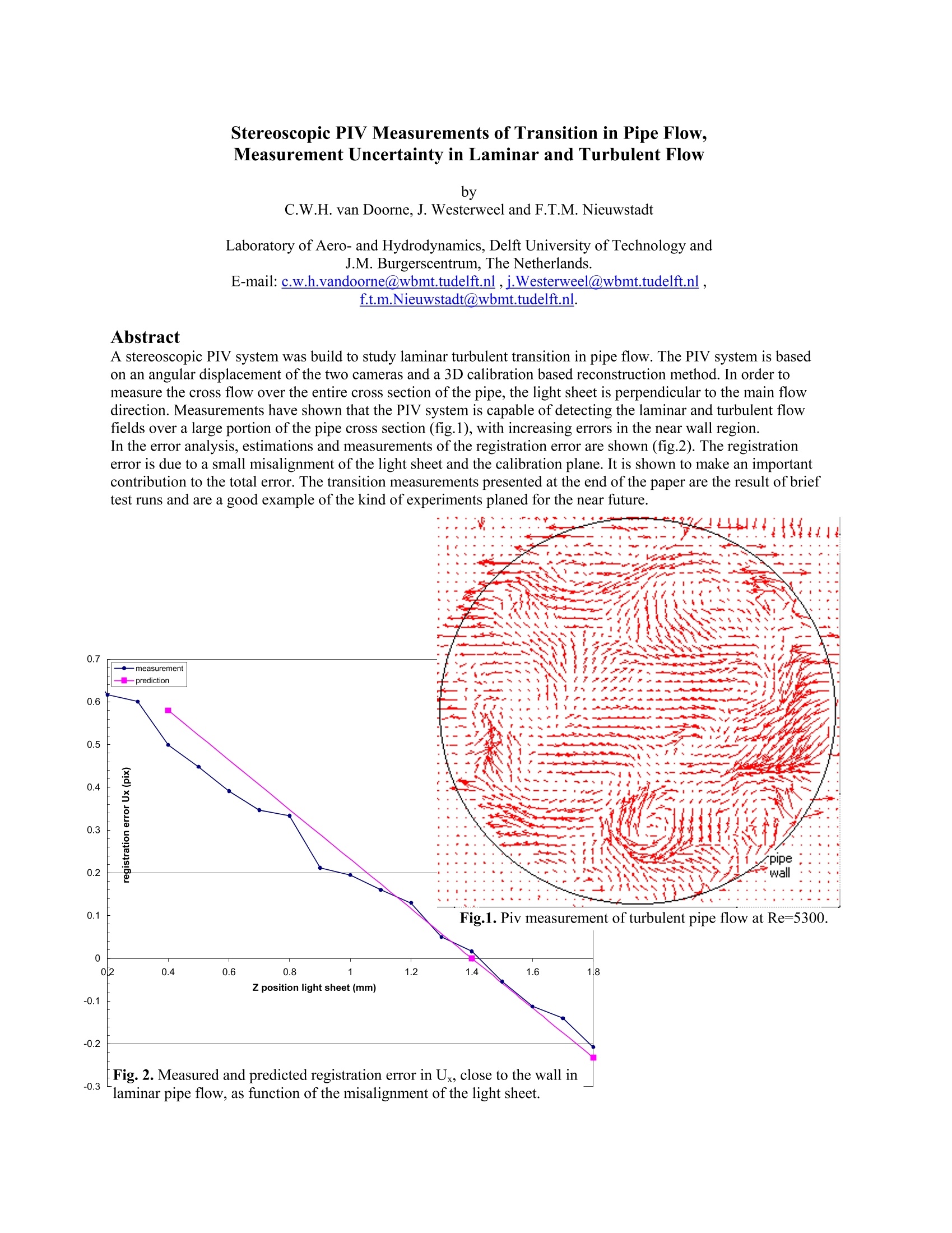
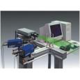
A stereoscopic PIV system was build to study laminar turbulent transition in pipe flow. The PIV system is based on an angular displacement of the two cameras and a 3D calibration based reconstruction method. In order to measure the cross flow over the entire cross section of the pipe, the light sheet is perpendicular to the main flow direction. Measurements have shown that the PIV system is capable of detecting the laminar and turbulent flow fields over a large portion of the pipe cross section (fig.1), with increasing errors in the near wall region.
In the error analysis, estimations and measurements of the registration error are shown (fig.2). The registration error is due to a small misalignment of the light sheet and the calibration plane. It is shown to make an important contribution to the total error. The transition measurements presented at the end of the paper are the result of brief test runs and are a good example of the kind of experiments planed for the near future.
方案详情

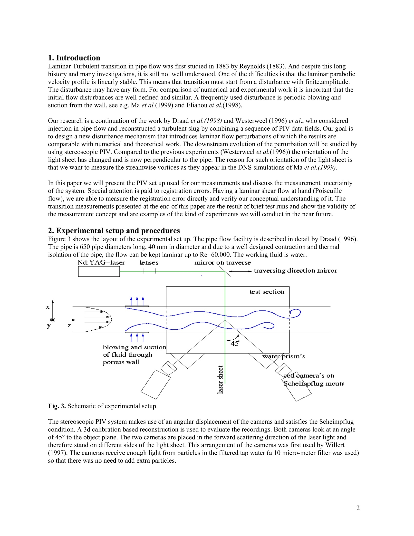
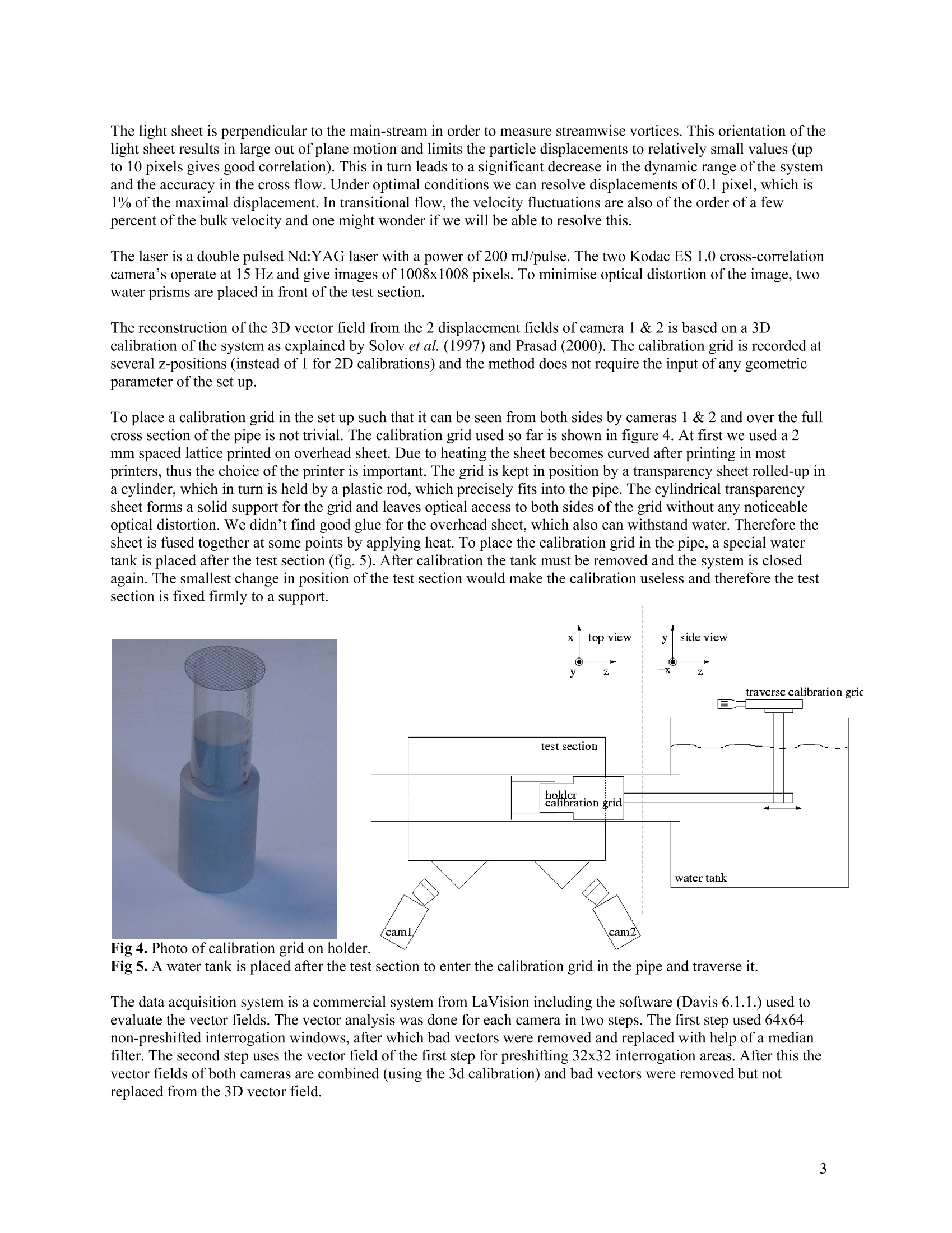
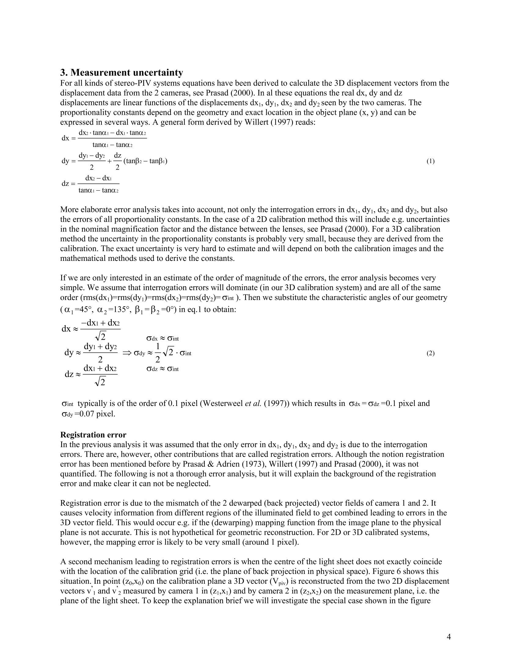
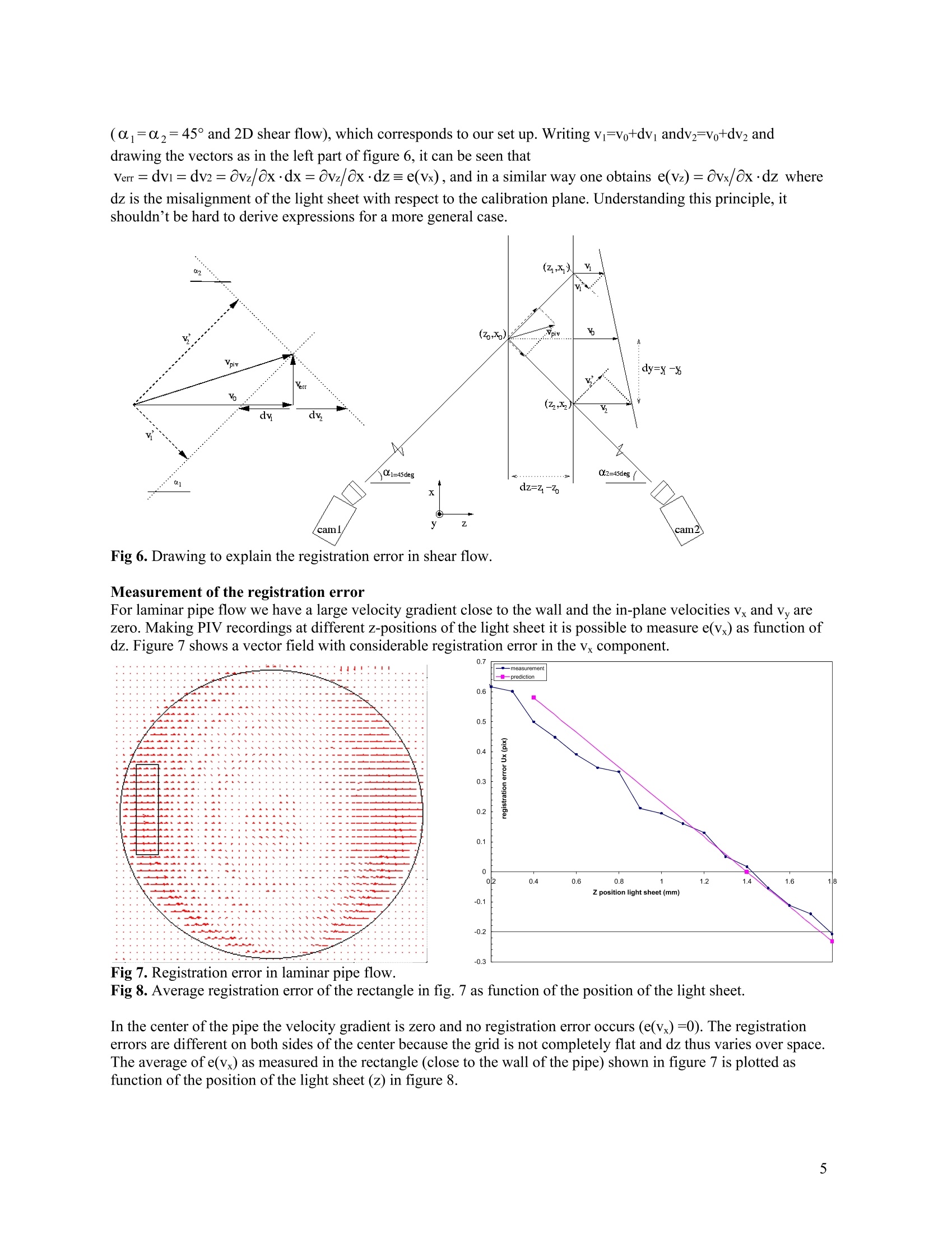
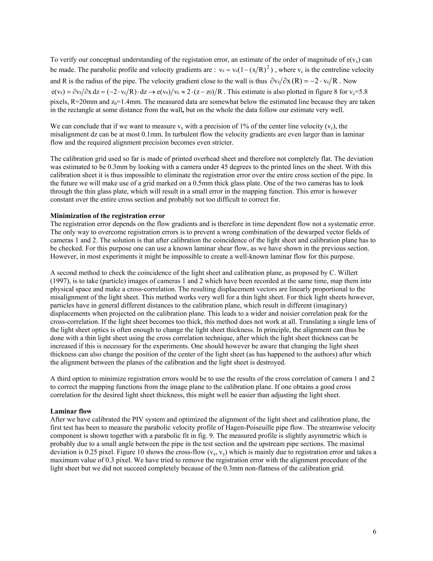
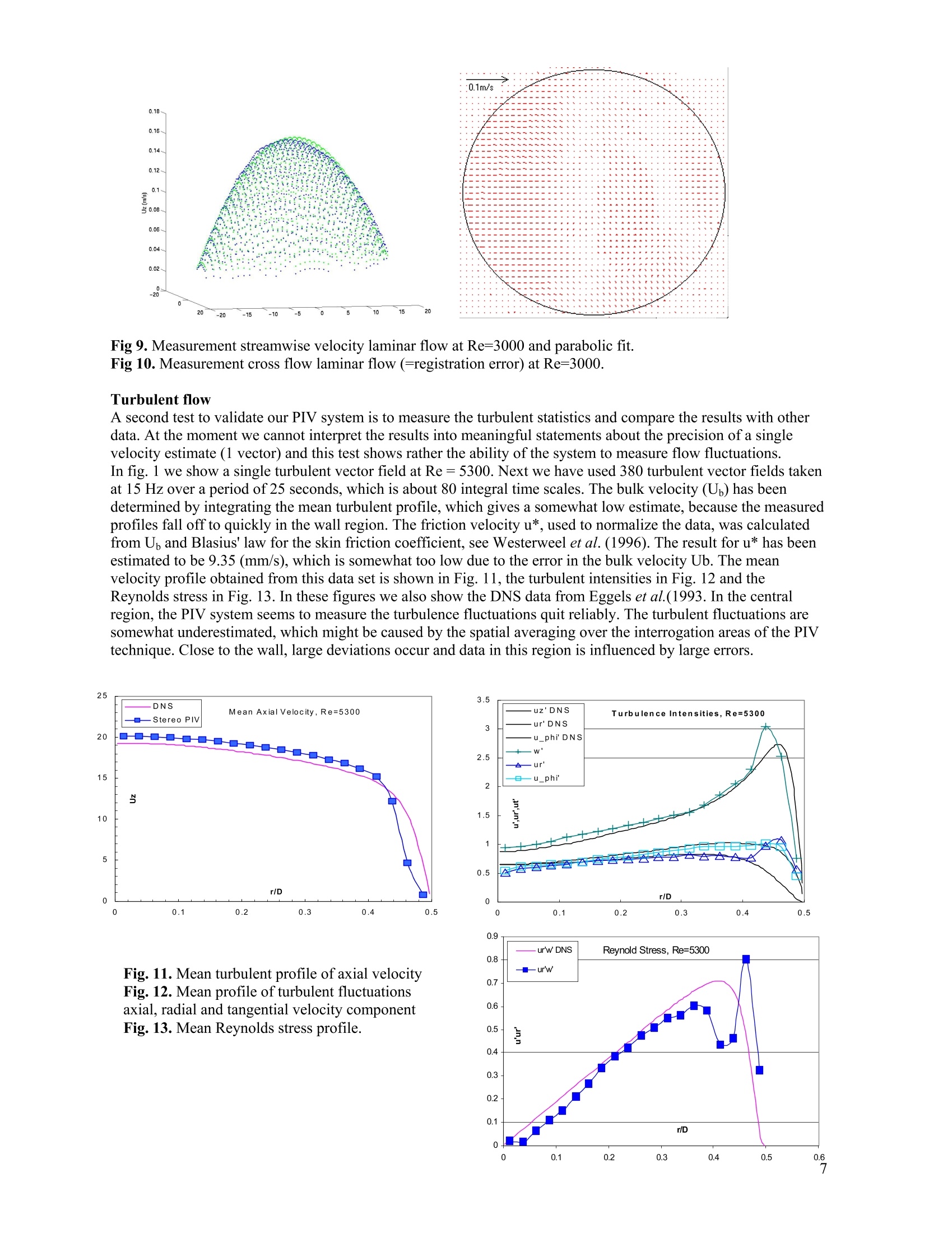
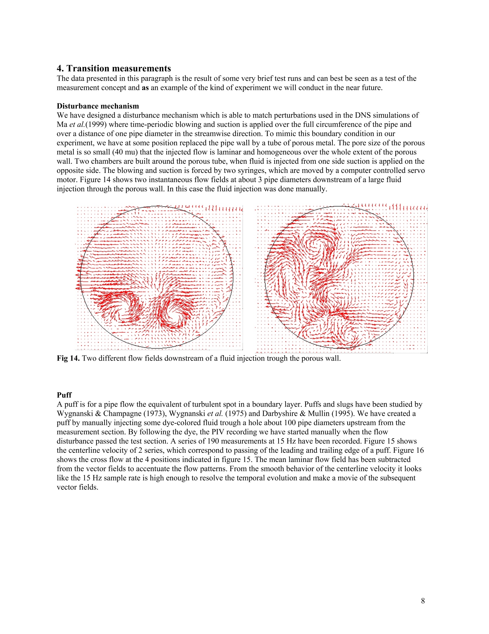
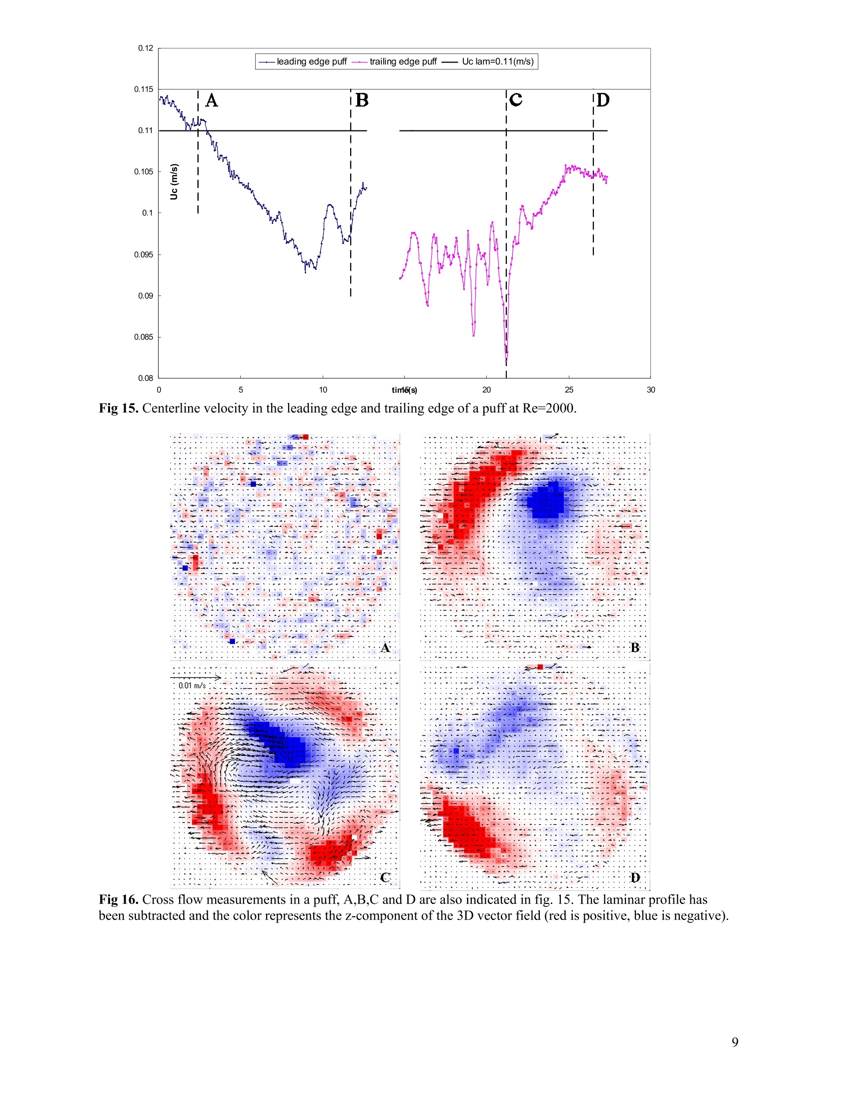
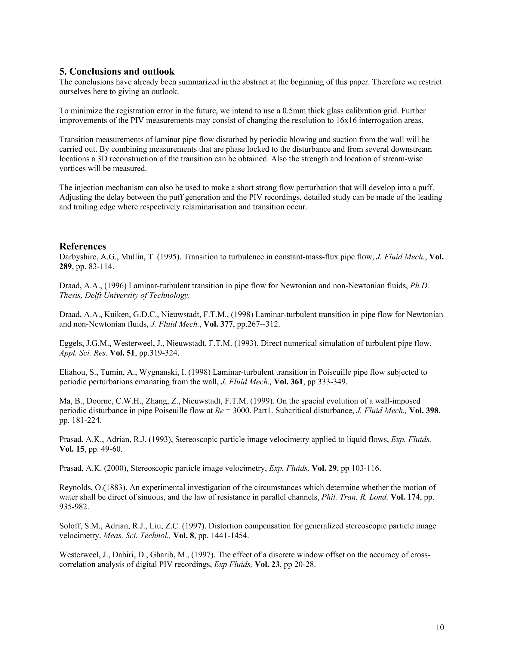
Stereoscopic PIV Measurements of Transition in Pipe Flow,Measurement Uncertainty in Laminar and Turbulent Flow by C.W.H. van Doorne, J. Westerweel and F.T.M. Nieuwstadt Laboratory of Aero- and Hydrodynamics, Delft University of Technology and J.M. Burgerscentrum, The Netherlands. E-mail:c.w.h.vandoorne@wbmt.tudelft.nl,j.Westerweel@wbmt.tudelft.nl, f.t.m.Nieuwstadt@wbmt.tudelft.nl. Abstract A stereoscopic PIV system was build to study laminar turbulent transition in pipe flow. The PIV system is basedon an angular displacement of the two cameras and a 3D calibration based reconstruction method. In order tomeasure the cross flow over the entire cross section of the pipe, the light sheet is perpendicular to the main flowdirection. Measurements have shown that the PIV system is capable of detecting the laminar and turbulent flowfields over a large portion of the pipe cross section (fig.1), with increasing errors in the near wall region.In the error analysis, estimations and measurements of the registration error are shown (fig.2). The registrationerror is due to a small misalignment of the light sheet and the calibration plane. It is shown to make an importantcontribution to the total error. The transition measurements presented at the end ofthe paper are the result of brieftest runs and are a good example of the kind of experiments planed for the near future. Fig.1. Piv measurement of turbulent pipe flow at Re=5300. -0.2 -0.3 Fig.2. Measured and predicted registration error in Ux, close to the wall inlaminar pipe flow, as function of the misalignment of the light sheet. 1. Introduction Laminar Turbulent transition in pipe flow was first studied in 1883 by Reynolds (1883). And despite this longhistory and many investigations, it is still not well understood. One of the difficulties is that the laminar parabolicvelocity profile is linearly stable. This means that transition must start from a disturbance with finite.amplitude.The disturbance may have any form. For comparison of numerical and experimental work it is important that theinitial flow disturbances are well defined and similar. A frequently used disturbance is periodic blowing andsuction from the wall, see e.g. Ma et al.(1999) and Eliahou et al.(1998). Our research is a continuation of the work by Draad et al.(1998) and Westerweel (1996) et al., who consideredinjection in pipe flow and reconstructed a turbulent slug by combining a sequence of PIV data fields. Our goal isto design a new disturbance mechanism that introduces laminar flow perturbations of which the results arecomparable with numerical and theoretical work. The downstream evolution of the perturbation will be studied byusing stereoscopic PIV. Compared to the previous experiments (Westerweel et al.(1996)) the orientation of thelight sheet has changed and is now perpendicular to the pipe. The reason for such orientation of the light sheet isthat we want to measure the streamwise vortices as they appear in the DNS simulations of Ma et al. (1999). In this paper we will present the PIV set up used for our measurements and discuss the measurement uncertaintyof the system. Special attention is paid to registration errors. Having a laminar shear flow at hand (Poiseuilleflow), we are able to measure the registration error directly and verify our conceptual understanding of it. Thetransition measurements presented at the end of this paper are the result of brief test runs and show the validity ofthe measurement concept and are examples ofthe kind of experiments we will conduct in the near future. 2. Experimental setup and procedures Figure 3 shows the layout of the experimental set up. The pipe flow facility is described in detail by Draad (1996).The pipe is 650 pipe diameters long, 40 mm in diameter and due to a well designed contraction and thermalisolation of the pipe, the flow can be kept laminar up to Re=60.000. The working fluid is water. Fig. 3. Schematic of experimental setup. The stereoscopic PIV system makes use of an angular displacement of the cameras and satisfies the Scheimpflugcondition. A 3d calibration based reconstruction is used to evaluate the recordings. Both cameras look at an angleof 45° to the object plane. The two cameras are placed in the forward scattering direction of the laser light andtherefore stand on different sides of the light sheet. This arrangement of the cameras was first used by Willert(1997). The cameras receive enough light from particles in the filtered tap water (a 10 micro-meter filter was used)so that there was no need to add extra particles. The light sheet is perpendicular to the main-stream in order to measure streamwise vortices. This orientation of thelight sheet results in large out of plane motion and limits the particle displacements to relatively small values (upto 10 pixels gives good correlation). This in turn leads to a significant decrease in the dynamic range of the systemand the accuracy in the cross flow. Under optimal conditions we can resolve displacements of 0.1 pixel, which is1% of the maximal displacement. In transitional flow, the velocity fluctuations are also of the order of a fewpercent of the bulk velocity and one might wonder if we will be able to resolve this. The laser is a double pulsed Nd:YAG laser with a power of 200 mJ/pulse. The two Kodac ES 1.0 cross-correlationcamera’s operate at 15 Hz and give images of 1008x1008 pixels. To minimise optical distortion of the image, twowater prisms are placed in front of the test section. The reconstruction of the 3D vector field from the 2 displacement fields of camera 1 & 2 is based on a 3Dcalibration of the system as explained by Solov et al. (1997) and Prasad (2000).The calibration grid is recorded atseveral z-positions (instead of 1 for 2D calibrations) and the method does not require the input of any geometricparameter of the set up. To place a calibration grid in the set up such that it can be seen from both sides by cameras 1 & 2 and over the fullcross section of the pipe is not trivial. The calibration grid used so far is shown in figure 4. At first we used a 2mm spaced lattice printed on overhead sheet. Due to heating the sheet becomes curved after printing in mostprinters, thus the choice of the printer is important. The grid is kept in position by a transparency sheet rolled-up ina cylinder, which in turn is held by a plastic rod, which precisely fits into the pipe. The cylindrical transparencysheet forms a solid support for the grid and leaves optical access to both sides of the grid without any noticeableoptical distortion. We didn’t find good glue for the overhead sheet, which also can withstand water. Therefore thesheet is fused together at some points by applying heat. To place the calibration grid in the pipe, a special watertank is placed after the test section (fig.5). After calibration the tank must be removed and the system is closedagain. The smallest change in position of the test section would make the calibration useless and therefore the testsection is fixed firmly to a support. Fig 4. Photo of calibration grid on holder. Fig 5. A water tank is placed after the test section to enter the calibration grid in the pipe and traverse it. The data acquisition system is a commercial system from LaVision including the software (Davis 6.1.1.) used toevaluate the vector fields. The vector analysis was done for each camera in two steps. The first step used 64x64non-preshifted interrogation windows, after which bad vectors were removed and replaced with help of a medianfilter. The second step uses the vector field of the first step for preshifting 32x32 interrogation areas. After this thevector fields of both cameras are combined (using the 3d calibration) and bad vectors were removed but notreplaced from the 3D vector field. 3. Measurement uncertainty For all kinds of stereo-PIV systems equations have been derived to calculate the 3D displacement vectors from thedisplacement data from the 2 cameras, see Prasad (2000). In al these equations the real dx, dy and dzdisplacements are linear functions of the displacements dx, dyi, dx2 and dy seen by the two cameras. Theproportionality constants depend on the geometry and exact location in the object plane (x, y) and can beexpressed in several ways. A general form derived by Willert (1997) reads: tandi-tana2 dx2-dxi More elaborate error analysis takes into account, not only the interrogation errors in dxi,dyi, dx and dy2, but alsothe errors of all proportionality constants. In the case of a 2D calibration method this will include e.g. uncertaintiesin the nominal magnification factor and the distance between the lenses, see Prasad (2000). For a 3D calibrationmethod the uncertainty in the proportionality constants is probably very small, because they are derived from thecalibration. The exact uncertainty is very hard to estimate and will depend on both the calibration images and themathematical methods used to derive the constants. If we are only interested in an estimate of the order of magnitude of the errors, the error analysis becomes verysimple. We assume that interrogation errors will dominate (in our 3D calibration system) and are all of the sameorder (rms(dxi)=rms(dyi)=rms(dx2)=rms(dy2)=Oint). Then we substitute the characteristic angles of our geometry(a=45,a2=135°,βi=B2=0°) in eq.1 to obtain: dx~ -dxi+ dx2 ddz~-xi+ dx2 Odz ≈ int √2 Oint typically is of the order of 0.1 pixel (Westerweel et al. (1997)) which results in Odx=Odz=0.1 pixel andOdy=0.07 pixel. Registration error In the previous analysis it was assumed that the only error in dx, dyi, dx and dy is due to the interrogationerrors. There are, however,other contributions that are called registration errors. Although the notion registrationerror has been mentioned before by Prasad & Adrien (1973), Willert (1997) and Prasad (2000), it was notquantified. The following is not a thorough error analysis, but it will explain the background of the registrationerror and make clear it can not be neglected. Registration error is due to the mismatch of the 2 dewarped (back projected) vector fields of camera 1 and 2. Itcauses velocity information from different regions of the illuminated field to get combined leading to errors in the3D vector field. This would occur e.g. if the (dewarping) mapping function from the image plane to the physicalplane is not accurate. This is not hypothetical for geometric reconstruction. For 2D or 3D calibrated systems,however, the mapping error is likely to be very small (around1 pixel). A second mechanism leading to registration errors is when the centre of the light sheet does not exactly coincidewith the location of the calibration grid (i.e. the plane of back projection in physical space). Figure 6 shows thissituation. In point (Zo,Xo) on the calibration plane a 3D vector (Vpiv) is reconstructed from the two 2D displacementvectors v and v 2 measured by camera 1 in (Zi,xi) and by camera 2 in (Z2,X2) on the measurement plane, i.e. theplane of the light sheet. To keep the explanation brief we will investigate the special case shown in the figure (a=02=45° and 2D shear flow), which corresponds to our set up. Writing Vi=Vo+dv andv2=Vo+dv2 anddrawing the vectors as in the left part of figure 6, it can be seen that Verr = dvi=dv2=Ovz/Ox·dx=0vz/Ox·dz=e(vx), and in a similar way one obtains e(vz)=0vx/Ox·dz wheredz is the misalignment of the light sheet with respect to the calibration plane. Understanding this principle, itshouldn’t be hard to derive expressions for a more general case. Fig 6. Drawing to explain the registration error in shear flow. Measurement of the registration error For laminar pipe flow we have a large velocity gradient close to the wall and the in-plane velocities v and vy arezero. Making PIV recordings at different z-positions of the light sheet it is possible to measure e(vx) as function ofdz. Figure 7 shows a vector field with considerable registration error in the vx component. Fig 7. Registration error in laminar pipe flow. Fig 8. Average registration error of the rectangle in fig. 7 as function of the position of the light sheet. In the center of the pipe the velocity gradient is zero and no registration error occurs (e(vx)=0). The registrationerrors are different on both sides of the center because the grid is not completely flat and dz thus varies over space.The average of e(vx) as measured in the rectangle (close to the wall of the pipe) shown in figure 7 is plotted asfunction of the position of the light sheet (z) in figure 8. To verify our conceptual understanding of the registation error, an estimate of the order of magnitude of e(vx) canbe made. The parabolic profile and velocity gradients are: Vz=Vc(1-(x/R)), where ve is the centreline velocityand R is the radius of the pipe. The velocity gradient close to the wall is thus 0vz/0x(R)=-2·ve/R. Nowe(vx)=0vz/0x dz=(-2·ve/R)·dz→e(vx)/Vc~2·(Z-Z0)/R. This estimate is also plotted in figure 8 for v=5.8pixels, R=20mm and zo=1.4mm.The measured data are somewhat below the estimated line because they are takenin the rectangle at some distance from the wall, but on the whole the data follow our estimate very well. We can conclude that if we want to measure vx with a precision of 1% of the center line velocity (ve), themisalignment dz can be at most 0.1mm. In turbulent flow the velocity gradients are even larger than in laminarflow and the required alignment precision becomes even stricter. The calibration grid used so far is made of printed overhead sheet and therefore not completely flat. The deviationwas estimated to be 0.3mm by looking with a camera under 45 degrees to the printed lines on the sheet. With thiscalibration sheet it is thus impossible to eliminate the registration error over the entire cross section of the pipe. Inthe future we will make use of a grid marked on a 0.5mm thick glass plate. One of the two cameras has to lookthrough the thin glass plate, which will result in a small error in the mapping function. This error is howeverconstant over the entire cross section and probably not too difficult to correct for. Minimization of the registration error The registration error depends on the flow gradients and is therefore in time dependent flow not a systematic error.The only way to overcome registration errors is to prevent a wrong combination of the dewarped vector fields ofcameras 1 and 2. The solution is that after calibration the coincidence of the light sheet and calibration plane has tobe checked. For this purpose one can use a known laminar shear flow, as we have shown in the previous section.However, in most experiments it might be impossible to create a well-known laminar flow for this purpose. A second method to check the coincidence of the light sheet and calibration plane, as proposed by C. Willert(1997), is to take (particle) images of cameras 1 and 2 which have been recorded at the same time, map them intophysical space and make a cross-correlation. The resulting displacement vectors are linearly proportional to themisalignment of the light sheet. This method works very well for a thin light sheet. For thick light sheets however,particles have in general different distances to the calibration plane, which result in different (imaginary)displacements when projected on the calibration plane. This leads to a wider and noisier correlation peak for thecross-correlation. If the light sheet becomes too thick, this method does not work at all. Translating a single lens ofthe light sheet optics is often enough to change the light sheet thickness. In principle, the alignment can thus bedone with a thin light sheet using the cross correlation technique,after which the light sheet thickness can beincreased if this is necessary for the experiments. One should however be aware that changing the light sheetthickness can also change the position of the center of the light sheet (as has happened to the authors) after whichthe alignment between the planes of the calibration and the light sheet is destroyed. A third option to minimize registration errors would be to use the results of the cross correlation of camera 1 and 2to correct the mapping functions from the image plane to the calibration plane. If one obtains a good crosscorrelation for the desired light sheet thickness, this might well be easier than adjusting the light sheet. Laminar flow After we have calibrated the PIV system and optimized the alignment of the light sheet and calibration plane, thefirst test has been to measure the parabolic velocity profile of Hagen-Poiseuille pipe flow. The streamwise velocitycomponent is shown together with a parabolic fit in fig. 9. The measured profile is slightly asymmetric which isprobably due to a small angle between the pipe in the test section and the upstream pipe sections. The maximaldeviation is 0.25 pixel. Figure 10 shows the cross-flow (Vx, Vy) which is mainly due to registration error and takes amaximum value of 0.3 pixel. We have tried to remove the registration error with the alignment procedure of thelight sheet but we did not succeed completely because of the 0.3mm non-flatness of the calibration grid. Fig 9. Measurement streamwise velocity laminar flow at Re=3000 and parabolic fit.Fig 10. Measurement cross flow laminar flow (=registration error) at Re=3000. Turbulent flow A second test to validate our PIV system is to measure the turbulent statistics and compare the results with otherdata. At the moment we cannot interpret the results into meaningful statements about the precision of a singlevelocity estimate (1 vector) and this test shows rather the ability of the system to measure flow fluctuations.In fig. 1 we show a single turbulent vector field at Re=5300. Next we have used 380 turbulent vector fields takenat 15 Hz over a period of 25 seconds, which is about 80 integral time scales. The bulk velocity (Ub) has beendetermined by integrating the mean turbulent profile, which gives a somewhat low estimate, because the measuredprofiles fall off to quickly in the wall region. The friction velocity u*, used to normalize the data, was calculatedfrom U and Blasius' law for the skin friction coefficient, see Westerweel et al. (1996). The result for u* has beenestimated to be 9.35 (mm/s), which is somewhat too low due to the error in the bulk velocity Ub. The meanvelocity profile obtained from this data set is shown in Fig. 11, the turbulent intensities in Fig. 12 and theReynolds stress in Fig. 13. In these figures we also show the DNS data from Eggels et al.(1993. In the centralregion, the PIV system seems to measure the turbulence fluctuations quit reliably. The turbulent fluctuations aresomewhat underestimated, which might be caused by the spatial averaging over the interrogation areas of the PIVtechnique. Close to the wall, large deviations occur and data in this region is influenced by large errors. 4. Transition measurements The data presented in this paragraph is the result of some very brief test runs and can best be seen as a test of themeasurement concept and as an example of the kind of experiment we will conduct in the near future. Disturbance mechanism We have designed a disturbance mechanism which is able to match perturbations used in the DNS simulations ofMa et al.(1999) where time-periodic blowing and suction is applied over the full circumference of the pipe andover a distance of one pipe diameter in the streamwise direction. To mimic this boundary condition in ourexperiment, we have at some position replaced the pipe wall by a tube of porous metal. The pore size of the porousmetal is so small (40 mu) that the injected flow is laminar and homogeneous over the whole extent of the porouswall. Two chambers are built around the porous tube, when fluid is injected from one side suction is applied on theopposite side. The blowing and suction is forced by two syringes,which are moved by a computer controlled servomotor. Figure 14 shows two instantaneous flow fields at about 3 pipe diameters downstream of a large fluidinjection through the porous wall. In this case the fluid injection was done manually. Fig 14. Two different flow fields downstream of a fluid injection trough the porous wall. Puff A puff is for a pipe flow the equivalent of turbulent spot in a boundary layer. Puffs and slugs have been studied byWygnanski & Champagne (1973), Wygnanski et al. (1975) and Darbyshire & Mullin (1995). We have created apuff by manually injecting some dye-colored fluid trough a hole about 100 pipe diameters upstream from themeasurement section. By following the dye, the PIV recording we have started manually when the flowdisturbance passed the test section. A series of 190 measurements at 15 Hz have been recorded. Figure 15 showsthe centerline velocity of 2 series, which correspond to passing of the leading and trailing edge of a puff. Figure 16shows the cross flow at the 4 positions indicated in figure 15. The mean laminar flow field has been subtractedfrom the vector fields to accentuate the flow patterns. From the smooth behavior of the centerline velocity it lookslike the 15 Hz sample rate is high enough to resolve the temporal evolution and make a movie of the subsequentvector fields. Fig 15. Centerline velocity in the leading edge and trailing edge of a puff at Re=2000. Fig 16. Cross flow measurements in a puff, A,B,C and D are also indicated in fig. 15. The laminar profile hasbeen subtracted and the color represents the z-component of the 3D vector field (red is positive, blue is negative). 5. Conclusions and outlook The conclusions have already been summarized in the abstract at the beginning of this paper. Therefore we restrictourselves here to giving an outlook. To minimize the registration error in the future, we intend to use a 0.5mm thick glass calibration grid. Furtherimprovements of the PIV measurements may consist of changing the resolution to 16x16interrogation areas. Transition measurements of laminar pipe flow disturbed by periodic blowing and suction from the wall will becarried out. By combining measurements that are phase locked to the disturbance and from several downstreamlocations a 3D reconstruction of the transition can be obtained. Also the strength and location of stream-wisevortices will be measured. The injection mechanism can also be used to make a short strong flow perturbation that will develop into a puff.Adjusting the delay between the puff generation and the PIV recordings, detailed study can be made of the leadingand trailing edge where respectively relaminarisation and transition occur. References Darbyshire, A.G., Mullin, T. (1995). Transition to turbulence in constant-mass-flux pipe flow, J. Fluid Mech., Vol.289, pp.83-114. Draad, A.A., (1996) Laminar-turbulent transition in pipe flow for Newtonian and non-Newtonian fluids, Ph.D.Thesis, Delft University ofTechnology. Draad, A.A., Kuiken, G.D.C., Nieuwstadt, F.T.M., (1998) Laminar-turbulent transition in pipe flow for Newtonianand non-Newtonian fluids, J. Fluid Mech., Vol. 377, pp.267--312. Eggels, J.G.M., Westerweel,J.,Nieuwstadt,F.T.M.(1993). Direct numerical simulation of turbulent pipe flow.Appl. Sci. Res. Vol. 51, pp.319-324. Eliahou, S., Tumin, A., Wygnanski, I. (1998)Laminar-turbulent transition in Poiseuille pipe flow subjected toperiodic perturbations emanating from the wall, J. Fluid Mech.,Vol. 361, pp 333-349. Ma, B., Doorne, C.W.H., Zhang, Z., Nieuwstadt, F.T.M. (1999). On the spacial evolution of a wall-imposedperiodic disturbance in pipe Poiseuille flow at Re=3000. Part1. Subcritical disturbance,J. Fluid Mech., Vol. 398,pp. 181-224. Prasad, A.K., Adrian, R.J. (1993), Stereoscopic particle image velocimetry applied to liquid flows, Exp. Fluids,Vol.15, pp. 49-60. Prasad, A.K. (2000), Stereoscopic particle image velocimetry, Exp. Fluids, Vol. 29,pp 103-116. Reynolds,O.(1883). An experimental investigation of the circumstances which determine whether the motion ofwater shall be direct of sinuous, and the law of resistance in parallel channels,Phil. Tran. R. Lond. Vol. 174, pp.935-982. Soloff,S.M., Adrian, R.J., Liu, Z.C. (1997). Distortion compensation for generalized stereoscopic particle imagevelocimetry. Meas. Sci. Technol., Vol. 8, pp. 1441-1454. Westerweel, J., Dabiri, D., Gharib, M., (1997). The effect of a discrete window offset on the accuracy of cross-correlation analysis of digital PIV recordings, Exp Fluids, Vol. 23, pp 20-28. Westerweel, J., Draad, A.A.(1996) Measurement of temporal and spatial evolution of transitional pipe flow withPIV, Development in laser techniques and fluid mechanics, 8" International Symposium, Lisbon, Portugal, 8-11Luly, 1996, pp.311-324. Westerweel, J., Draad, A.A., van der Hoeven,J.G.Th., van Oord, J. (1996). Measurement of fully-developedturbulent pipe flow with digital particle image velocimetry, Exp.Fluids, Vol 20, pp. 165-177. Willert, C. (1997). Stereoscopic digital particle image velocimetry for application in wind tunnel flows. Meas. Sci.Technol., Vol. 8, pp1465-1479. Wygnanski, I.J., Champagne, F.H. (1973). On transition in a pipe. Part 1. The origin of puffs and slugs and theflow in a turbulent slug. J Fluid Mech, Vol. 59,pp. 281-335. Wygnanski, I., Sokolov, M., Friedman, D. (1975).On transition in a pipe. Part 2. The equilibrium puff. J FluidMech., Vol.69, pp. 283-304.
确定
还剩9页未读,是否继续阅读?

北京欧兰科技发展有限公司为您提供《流体中速度矢量场检测方案(粒子图像测速)》,该方案主要用于其他中速度矢量场检测,参考标准--,《流体中速度矢量场检测方案(粒子图像测速)》用到的仪器有三维立体PIV
推荐专场


相关方案
更多
该厂商其他方案
更多