流体中速度场,浓度场检测方案(粒子图像测速)

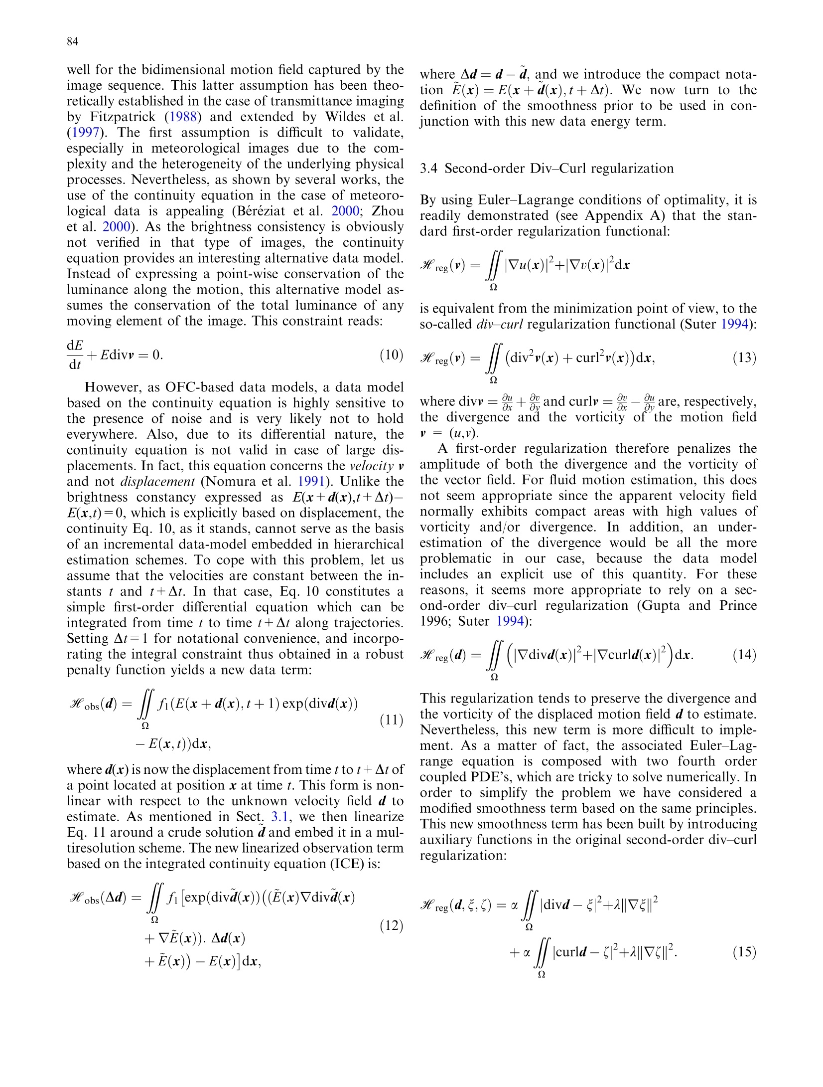
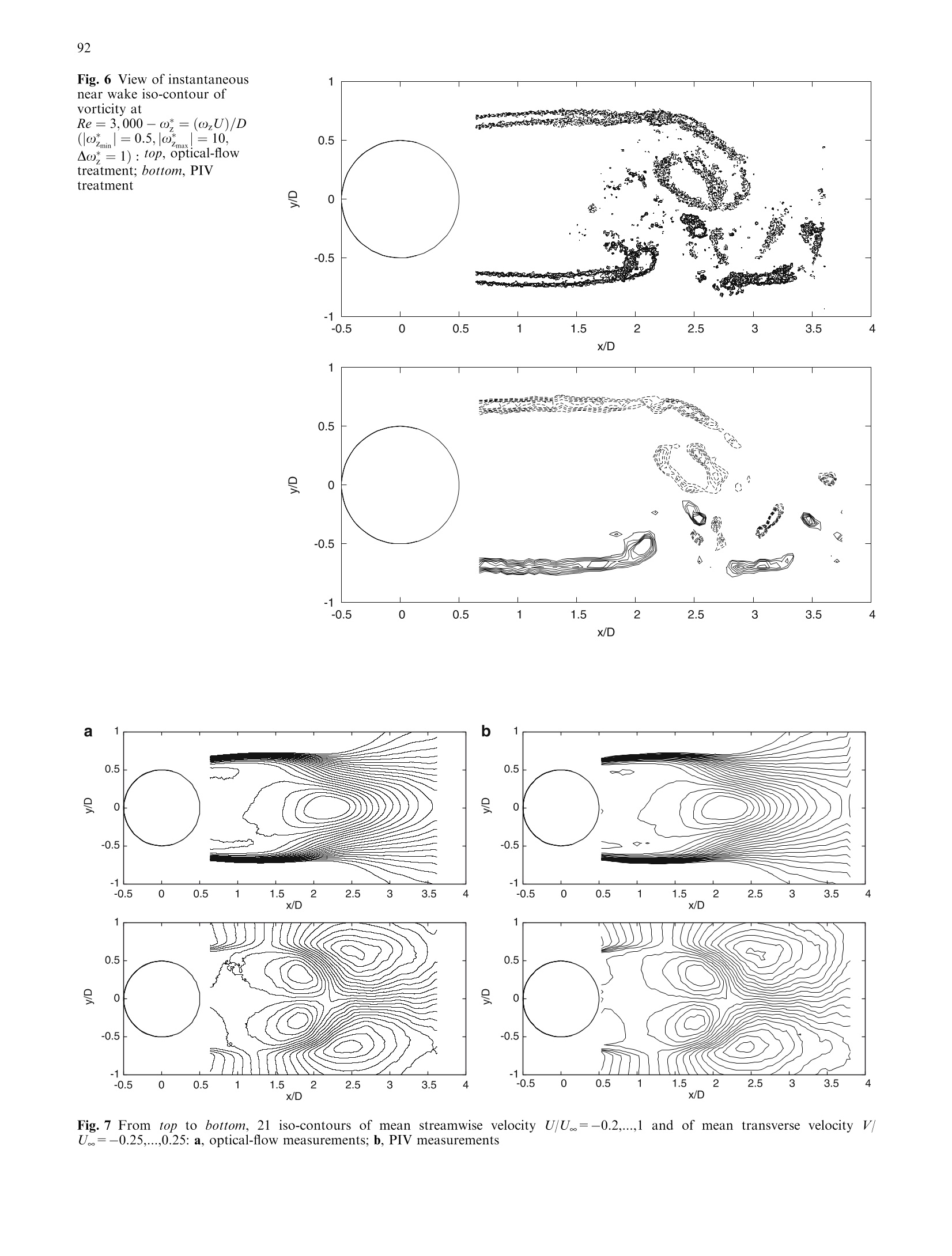
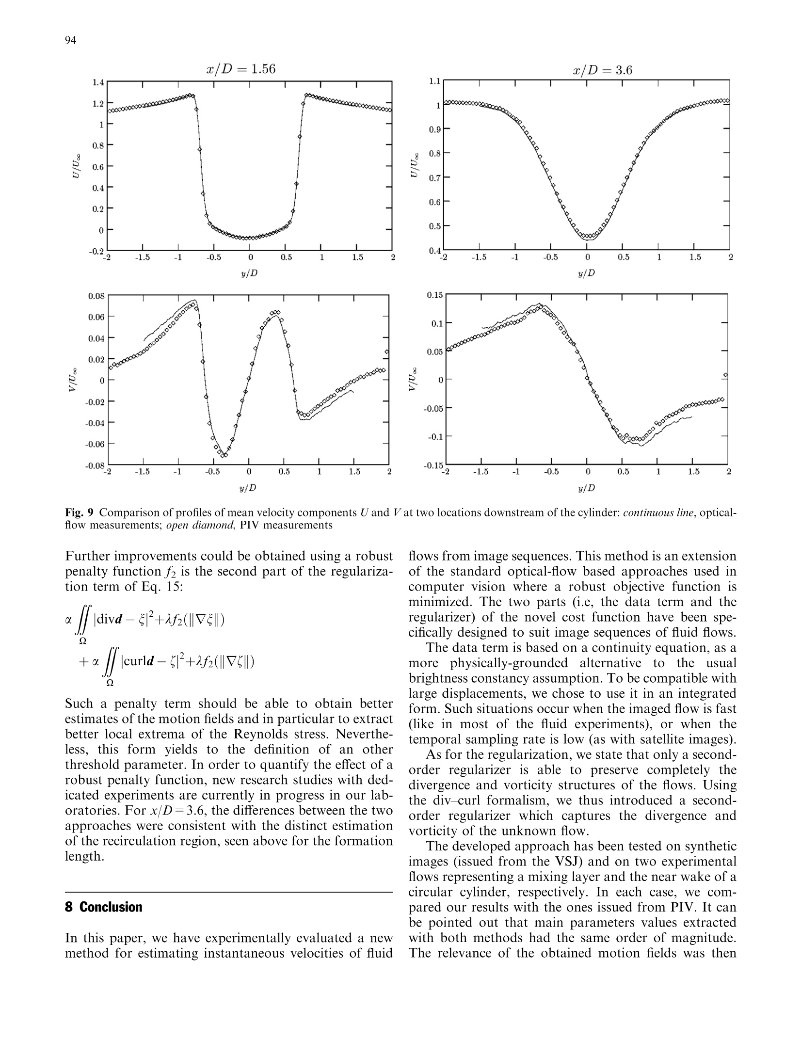
Experiments in Fluids (2006) 40： 80-97DOI 10.1007/s00348-005-0048-yRESEARCH ARTICLE 81 T. Corpetti· D. Heitz ·G. Arroyo·E. Memin A. Santa-Cruz Fluid experimental flow estimation based on an optical-flow scheme Abstract We present in this paper a novel approach ded-icated to the measurement of velocity in fluid experimentalflows through image sequences. Unlike most of themethods based on particle image velocimetry (PIV) ap-proaches used in that context， the proposed technique is anextension of“optical-flow”schemes used in the computervision community， which includes a specific enhancementfor fluid mechanics applications. The method we proposeenables to provide accurate dense motion fields. Itincludesan image based integrated version of the continuityequation. This model is associated to a regularizationfunctional， which preserve divergence and vorticity blobsof the motion field. The method was applied on syntheticimages and on real experiments carried out to allow athorough comparison with a state-of-the-art PIV methodin conditions of strong local free shear. Keywords Fluid motion measurement· Continuityequation · Div-curl regularization ·Optical-flow· PIV 1 Introduction In the experimental fluid mechanics domain， imagingtechniques now routinely produce various types of vid-eos which constitute a unique source of information forboth applied and theoretical studies (Adrian 11991：Wallace and Foss 1995； Wernert et al. 1996). In such acontext， cameras provide in a versatile and non-intrusive ( T. Corpetti () . D . H eitz· G . Arroyo· A. Santa-Cruz ) ( Cemagref 17， a venue de Cucille， ) ( 35044 R ennes Cedex， F rance ) E-mail： thomas.corpetti@uhb.fr E. MeminIRISA/INRIA Campus， Universitaire de Beaulieu， 35042 Rennes Cedex， France Present address： T. CorpettiLaboratoire COSTEL UMR 6554 LETG. Maison de la Recherche.Place du Recteur Henri Le Moal. 35043 Rennes Cedex， France way huge amounts of (almost) continuous spatio-tem-poral data， as opposed to in situ measurement techniques(e.g.， thermal anemometry)， which supply only sparsespatial information. On the other hand， unlike dedicatedprobes， images only give indirect access to the physicalquantities of interest. With videos or image series， onemust face the complex task of extracting these quantitiesfrom the intensity patterns recorded in the successiveimages. As compared to more classical motion analysisproblems addressed by the computer vision community，the analysis of fluid motion from images is particularlychallenging due to the great deal of spatial and temporaldistortions that the intensity patterns exhibit. In most of the domains requiring experimental fluidflow visualization and measurement， particle image ve-locimetry (PIV) techniques or related methods play animportant role and are intensively used to provide motionestimation. These techniques are based on a spatio-tem-poral cross-correlation submittedto2aconsistencyassumption of the flow within a local interrogation win-dow. Theinterrogation windows generally contain severalparticles with different motions. Considering a uniquemotion vector for all these particles may lead in somecircumstances to a very poor local motion representation. In the computer vision community， obtaining the“optical flow”consists in extracting a dense representa-tion of the motion field (i.e. one vector per pixel). Most ofthese methods are based on a formulation introduced byHorn and Schunck (1981) in the early 80s， and consist inestimating a vectorial function by minimizing an objectivefunctional. This functional is composed of two terms； thedata model and a regularization term. The former is anadequacy term between the unknown motion functionand the data. It generally relies on a brightness consistencyassumption. Similarly to correlation techniques， thisassumption states that a given point keeps its intensityalong its trajectory. The latter promotes a globalsmoothness of the motion field over the image. It must bepointed out that these techniques have been devised forthe analysis of quasi-rigid motions with stable salientfeatures. Unfortunately， there is no such thing as an “object”in most imaged fluid flows which contain mainlydeformable and transient brightness patterns. On thesesequences， techniques based on standard computer visioningredients are thus intrinsically limited. The design ofalternative approaches dedicated to fluid motion thusremains a widely open research domain. In this paper， we propose an optical-flow methodwhich permits to extract reliable dense motion fields.This method is dedicated to the analysis of image se-quences of fluid flows. It includes， in the data-modelterm and in the smoothness term， specific adaptationsconsistent with the physics of flow motion. This article is organized as follows. In the first section，we present the conventional approaches frequently usedby the fluid mechanics community to extract velocitymeasurements from PIV images. Then， in the secondsection， we present the proposed alternative. In the lastsection， results from synthetic images and experiments ontwo classical flows， a mixing layer and the near wake of acircular cylinder， are presented and analysed. We providesome elements of comparison of our method with a state-of-the-art commercial PIV system. 2 PIV approaches 2.1 Overview Particle image velocimetry methods are mainly used influid mechanics for their known advantages (non-intru-sive sensor， ability to obtain relevant instantaneousvelocity fields，...). The idea is to visualize， through alaser sheet pulse associated to a camera， a plane area ofthe flow sowed with luminescent/illuminated particles. Atemporal correlation analysis of the images providesmotion measurements of the observed particles. Unlikededicated probes which are able to obtain directly thedesired measurements， the velocity is here extractedfrom the brightness information of the image sequence. Since the 70s， numerous methods have been proposedto extract velocity fields from particle images. See forinstance (Adrian 1991； Raffel et al. 2000) for an ex-tended bibliography on the subject. In the next sections，we will further describe common PIV approaches. 2.2 Computation of the motion field in PIV systems Most of the PIV systems rely on correlation functionssuch as “auto-correlation”(if only one image containingthe traces of particles is available) or“cross-correlation”(if the temporal information is separated in two images).This latter technique is usually preferred， due to its betterstability against noise.The image frames are interrogatedby the computation of the spatial cross-correlation in anM × N interrogation region： where I and I2 are the first and second discrete imageframes，w(x) being a window centered on the point x.The motion associated to the centre of the interrogationwindow d(x) = (u(x)，v(x)) corresponds to a peak of thecorrelation surface. Three main options are available to compute thecorrelation surface Eq. ： l. Direct computation： this method requires (M×N)multiplications and additions for an (M ×N) inter-rogation window and is thus expensive in computa-tion time： 2. Computation in the Fourier domain： this technique isused to accelerate the previous processing and tolocalize easily the correlation peak. Unfortunately，one difficulty of this approach is the lack of flexibilitybetween the Fourier domain and the physical one，especially for post-processing treatment； 3. Computation in the spectral domain with physicalpost-processing using the Wiener-Khintchine theoremthat permits a fast come back in the physical domain As they lead to real time computations， the secondand third options (computation in the Fourier space) aremainly used in PIV. Let us notice that to prevent fromaliasing artefacts， Nyquist criteria must be respected： theconsidered displacement d is then such that d<(N/2，M/2) pixels. Hence， if necessary， an underestimation ofthe velocity magnitude is commonly performed bygrowing up the size of the interrogation window or bydecreasing the time interval between two laser pulses.This manipulation may affect significantly the quality ofthe estimated motion field and a compromise has to begenerally defined between a direct computation whichdoes not have such restrictions and a fast computationin the Fourier space (McKenna and McGillis 2002). Another difficulty inherent to correlation methods liesin the discrete data nature. As a matter of fact， with suchapproaches the estimated displacement vector is intrinsi-cally discretized on the image grid (i.e. vectors of the typed= uxpix，v× pix)， where u and v are integers and pix isthe pixel size). Infinitesimal brightness variation can in-deed not be identified. This results in the well known“peak-locking”effect which spoils the accuracy of thevelocity measurement. Many studies have been done toattenuate this phenomenon. One possibility consists inincreasing particle size (which effective particle image sizemust be two or three pixels) or to pay a particular atten-tion to the correlation maxima localization (by soundinterpolations for example). Several methods have beenproposed to provide“sub-pixel”accuracy (Lourenco andKrothapalli 1995； Willert and Gharib 1991). Actually， many extensions of the basic cross-correla-tion principle have been proposed to improve the esti-mation quality in terms of dynamic range， accuracy andspatial resolution. For example Scarano and Reithmuller(2000) and Lecuona et al. (2002) used an iterative pre-diction of the unknownvelocity in the estimationscheme， whereas Lourenco and Krothapalli (2000) or Wereley and Meinhart (2001) directly modified the cor-relation criterion， using a central difference approxima-tion (of second order) instead of a forward differenceapproximation (of first order) as commonly done. Onecan also note that the use of a super-resolution techniqueasin Nogueiraeet al. (2001) allows an uncertaintyreduction and attenuates the effect of peak-locking. 2.3 Discussion Many studies on cross-correlation methods have beendone and many methods enabling to extract relevantmotion information are available. Even if the principleof correlation techniques enables to extract only dis-placement vectors on the image lattice， many extendedmethods have been proposed to achieve“sub pixel”accuracy. All these correlation techniques share never-theless some common limitations whichpreventsacomfortable use (Lourenco and Krothapalli 2000)： 1. Due to the finite size of the interrogation area andparticle drop out， a “loss of pairing”may alter theestimation. In this case， the maximum of correlationdoes not correspond to the actual motion. The defi-nition of the size of the interrogation window is in-deed very problematic to extract a relevant motion inaccordance with the observed phenomenon； 2. The existence of“velocity and speeding gradient in theinterrogation region” introduces a bias towards thelower displacements and higher seeded sub-regions as aresult of the more frequent pairings. For large interro-gation windows， this is very problematic. It is never-theless important to note that this can be (at leastpartially) overcome using variable size windows anddeformable grids (Scarano and Reithmuller 2000)； 3. Due to its statistical nature， only the “most proba-ble”displacement is extracted for each interrogationwindow. All these limitations can hardly be avoided as they areintrinsically linked to the discrete and local nature ofcorrelation methods. Optical-flow approaches， originally introduced byHorn and Schunck (1981)， enable to extract in a naturalway a dense motion field (i.e. one vector per pixel). Suchtechniques take into account the whole image to esti-mate a vectorial continuous function representing thevelocity field. As a consequence they are intrinsicallyable to avoid the difficulties mentioned above. The ideawhich consists of using optical-flow methods for PIVimages appears then very attractive. Unfortunately suchtechniques designed for computer vision applicationshave also some limitations， which prevents their directuse in an experimental fluid mechanics context. In the following section， we give more details on thebasis of generic optical-flow schemes. We then discusstheir limitations with respect to fluid image sequencesand present our extension of these techniques， specifi-cally dedicated to fluid flows velocity measurements. 3 Optical-flow scheme Obtaining the optical flow consists in estimating a densemotion field from two consecutive images. As previouslymentioned， many methods have been proposed in the lasttwo decades to estimate such an optical flow. Most ofthemare based on the seminal work of Horn and Schunck(1981). In this section，optical-flow methods will then referto this latter definition. It is nevertheless important topoint out that some authors propose reliable optical-flowcomputations not based on Horn and Schunck (1981)，especially for PIV images in Quenotet al. (1998)where theauthors use dynamic programming and orthogonalalgorithms. The reader will find in Barron et al. (1994) asurvey of different methods for computing optical flow(differential techniques， region based matching， energybased methods and phase based techniques). 3.1 Generic optical-flow estimator The most accurate techniques to address the genericproblem of estimating the apparent motion from imagesequences are based on the seminal work by Horn andSchunck (1981). These techniques are based on theminimization of a global cost function composed oftwo terms. The first one， named“observation term”， isderived from a brightness constancy assumption andassumes that a given point keeps the same intensityalong its trajectory. It is expressed through the wellknown optical flow constraint equation (OFCE)： where w(x，t)= (u，v) is the unknown velocity field attime t and location x= (x，y) in the image plane Q，E(x，t) is the image brightness， viewed for a while as acontinuous function. This first term relies on theassumption that the visible points conserve roughly theirintensity in the course of a small displacement. This single (scalar) observation term does not allowto estimate the two components u and v of the velocity.In order to solve this ill-posed problem， it is common toemploy an additional smoothness constraint reg.Usually， this second term enforces a spatial smoothnesscoherence of the flow field. It relies on a contextual assumption which enforces a spatial smoothness of thesolution. This term usually reads： As with the penalty function in the data term， the penaltyfunction f2 was taken as a quadratic in early studies， but asofter penalty is now preferred in order not to smooth outthe natural discontinuities (boundaries，...) of the velocityfield (Black 1994； Cohen and Herlin 1999； Kornprobstet al. 1999； Memin and Perez 1998). Based on Eqs. 2 and4， the estimation of motion can be done by minimizing： where a>0 is a parameter controlling the balance be-tween the smoothness constraint and the global ade-quacy to the observation assumption. Due to its differential nature， the relation in Eq. 2 isonly defined for infinitesimal displacements. To handlelarge displacements it is common to use the expressionEq. 2 of the brightness conservation in an integrated way： where At is the temporal sampling rate and d(x) is thedisplacement from time t to t+At of the point located atposition x at time t. This new form， valid whatever themagnitude of d(x) be， is however highly nonlinear in theunknown vector. As a consequence， almost all studiesresort to a succession of linearizations around a previousestimate d(x)d(d)d(x) (d(x)=d(x)d(d)d(x)+Ad(x))embedded1 within a multiresolution scheme (using abilinar interpolationfor the projection)..The newcost-function to be minimized with respect to thedisplacement increment Adreads then： The associated successive minimizations are usuallyperformed using efficient iterative methods (Memin andPerez 1998， 2002). It is important to outline that such an estimator de-fined as the minimizer of is generic. It is only basedon the assumption of luminance conservation and offirst-order spatial smoothness of the motion. Even if thiskind of estimator has been successfully used for fluidmotion (Bannehr et al. 1996； Cohen and Herlin 1999；Larsen et al. 1998； Memin and Perez 1999；Ruhnauet al. 2005； Wallace and Foss1995)， the underlying assumptions are far from being sound hypothesis forsuch an applicative domain. As a matter of fact， imagesequences representing fluid phenomena exhibit areaswhere the luminance function undergoes high temporalvariations along the motion. These areas are often thecentreoftridimensional motionsithatcause theappearance or the disappearance of fluid matter withinthe bidimensional visualization plane. These regions arein addition associated to divergent motions whichinfluence greatly the shape of the velocity field in largesurrounding areas. An accurate estimation of the 2Dapparent motion in such regions is therefore of thehighest importance and isIShardly possible with1(theoptical-flow constraint. 3.2 Fluid dedicated optical-flow estimator In a recent paper Corpetti et al. (2002) proposed anoptical-flow technique specifically dedicated to imagesequences depicting fluid flow phenomenona. This spe-cialized optical-flow estimator relies on an adaptation ofthe functional data model and smoothness term. 3.3 Continuity equation and data model Insteadof sticking too tthee intensity(conservationassumption， the data model that has been consideredrelies on the continuity equation： where x denotes the density of the fluid， v its 3D velocityand divy=++ stands for the divergence of thevector field p=(u，v，w). Simple manipulations yield thealternative writing： When the divergence of the 3D apparent flow vanishes，this equation is of the same form as the 2D optical flowconstraint on luminance. The continuity equation， orig-inally introduced in Schunk (1984) as a data model formotion estimation of intensity time varying images， hasbeen since incorporated in several works. It has beenconsidered in the context of fluid imagery either forsatellite meteorological images (Bereziat et al. 2000；Corpetti et al. 2002；Zhou et al. 2000) or for experi-mental fluid mechanics (Wildes et al. 1997). It has alsobeen introduced in medical imaging domain to recover3D deformation fields of the heart (Song and Leahy1991) or to analyse blood flow (Amini 1994). In all thesecases， this model has been proved to represent an alter-native to standard luminance constancy assumption. The use of continuity equation for image sequencesanalysis relies on two hypotheses. First， the luminancefunction is assumed to be directly related to a passivequantity transported by the fluid. Secondly， the conti-nuity equation which holds in 3D， is assumed to hold as well for the bidimensional motion field captured by theimage sequence. This latter assumption has been theo-retically established in the case of transmittance imagingby Fitzpatrick (1988) and extended by Wildes et al.(1997). The first assumption is difficult to validate，especially in meteorological images due to the com-plexity and the heterogeneity of the underlying physicalprocesses. Nevertheless， as shown by several works， theuse of the continuity equation in the case of meteoro-logical data is appealing (Bereziat et al. 2000； Zhouet al. 2000). As the brightness consistency is obviouslynot verified in that type of images， the continuityequation provides an interesting alternative data model.Instead of expressing a point-wise conservation of theluminance along the motion， this alternative model as-sumes the conservation of the total luminance of anymoving element of the image. This constraint reads： However， as OFC-based data models，a data modelbased on the continuity equation is highly sensitive tothe presence of noise and is very likely not to holdeverywhere. Also， due to its differential nature， thecontinuity equation is not valid in case of large dis-placements. In fact， this equation concerns the velocity vand not displacement (Nomura et al. 1991). Unlike thebrightness constancy expressed as E(x+d(x)，t+At)-E(x，t)=0， which is explicitly based on displacement， thecontinuity Eq. 10， as it stands，cannot serve as the basisof an incremental data-model embedded in hierarchicalestimation schemes. To cope with this problem， let usassume that the velocities are constant between the in-stants t and t+At. In that case， Eq. 10 constitutes asimple first-order differential equation which can beintegrated from time t to time t+At along trajectories.Setting At=1 for notational convenience， and incorpo-rating the integral constraint thus obtained in a robustpenalty function yields a new data term： where d(x) is now the displacement from time t to t+At ofa point located at position x at time t. This form is non-linear with respect to the unknown velocity field d toestimate. As mentioned in Sect. 3.1， we then linearizeEq. 11 around a crude solution d and embed it in a mul-tiresolution scheme. The new linearized observation termbased on the integrated continuity equation (ICE) is： where Ad=d-d， and we introduce the compact nota-tion E(x)=E(x+d(x)，t+At). We now turn to thedefinition of the smoothness prior to be used in con-junction with this new data energy term. 3.4 Second-order Div-Curl regularization By using Euler-Lagrange conditions of optimality， it isreadily demonstrated (see Appendix A) that the stan-dard first-order regularization functional： is equivalent from the minimization point of view， to theso-called div-curl regularization functional (Suter 1994)： where divv=+" and curlv=&- are， respectivelythe divergence and the vorticity of the motion fieldv=(u，V). A first-order regularization therefore penalizes theamplitude of both the divergence and the vorticity ofthe vector field. For fluid motion estimation， this doesnot seem appropriate since the apparent velocity fieldnormally exhibits compact areas with high values ofvorticity and/or divergence. In addition， an under-estimation of the divergence would be all the moreproblematic in our case， becausethe data modelincludess an explicitt use of this quantity. For thesereasons， it seems more appropriate to rely on a sec-ond-order div-curl regularization (Gupta and Prince1996； Suter 1994)： This regularization tends to preserve the divergence andthe vorticity of the displaced motion field d to estimate.Nevertheless， this new term is more difficult to imple-ment. As a matter of fact， the associated Euler-Lag-range equation is composed with1 two fourth ordercoupled PDE’s， which are tricky to solve numerically. Inorder to simplify the problem we have considered amodified smoothness term based on the same principles.This new smoothness term has been built by introducingauxiliary functions in the original second-order div-curlregularization： We now turn to the minimization issue of the wholeenergy function M=Xobs +a reg. Two main sets ofvariables have to be estimated. The first one is the mo-tion field d， and the second one consists in the two scalarfields and. The estimation is conducted alternativelyby minimizing 光obs +areg with respect to d，i and ： For the motion field d， the use of a robust penaltyfunction in the observation term yields to an iterativelyre-weighted least squares minimization with the estima-tion of outliers data z (see Appendix B). Concerningand ， we have a linear least-square problem. A Gauss-Seidel solver was used for all linear least-square mini-mizations. The process is considered to be finished whenthe relative change in the L2-norm of Ad is below 1%. The minimization process is summarized below： Let us now have a particular attention to the minimi-zation w.r.t the motion field ▲d (first Eq. 17). For betterand faster convergence， the minimization with respect tothe incremental displacement field Adat a given resolutionis performed using the coarse-to-fine multi-parametricmultigrid framework technique introduced in Memin andPerez (1998). More precisely， the motion is constrained to bepiecewise-parametric relatively to an image partitionwhich becomes finer and finer. At a “grid”level (namedl)， the pixel grid is partitioned in blocks Bn of size2×2， and the increment field is constrained to satisfy achosen parametric model. In practice， until the penulti-mate grid level， the affine parametrization is chosen00(i.e：(u，u)=)oo1xo). The last levelyl=0 corresponds to the pixel grid itself： when it is finallyreached， no parametric constraint applies anymore. Ateach given level， the cost terms to be minimized must berewritten in function of the parameter vectors (⑧). Thissymbolic rewriting is explained in Memin and Pérez(1998). The estimation at the coarsest grid-level is fast be-cause the space of solutions is of reduced dimension. Itserves as a reliable initialization for the next level，yielding to this new computation more efficiency， and soon until the pixel grid itself. The combination of the multiresolution and themultigrid techniques partly makes possible to preventfrom stopping the process of minimization in a localminimum. 4 Experimental details 4.1 VSJ standard image-pairs The visualization society of Japan (VSJ) developed in1999 PIV standard images and PIV guide tools in orderto popularize the PIV techniques. Within this project，many synthetic PIV image sequences called “standardimages”， were generated along with the correspondingground truth velocity vector fields in a wide variety ofcontrolled conditions (Okamoto et al. 2000). They areavailable on the internet. The parameters of the eightstandard situations tested in this paper are listed in Ta-ble 1 and represent： the number N of particles that arepresent in the images， the particle diameter Dm associatedto its standard deviation Ds， the average image velocityVm and the out-of-plane velocity Wm. Compared to imagepair #1， the pairs #2 and #3 differ only with respect to themagnitude of the flow field； the image pairs #4 and #5have only different number of particle； the pairs #6 and#7 have particles with a different diameter while the pair#8 has a high out of plane velocity. relative Li norm error (Li norm of the differencebetween the correct and computed velocities in pixels/frame divided by the average in-plane velocity) tocompare the different motion fields. 4.2 Plane turbulent mixing layer The mixing layer studied here has been generated in aclosed circuit， subsonic wind tunnel R300 of the Centred'Etudes Aerodynamiques et Thermiques， University ofPoitiers， France (CEAT). Thiswind tunnel hassiasquareetest sectionofcross-sectional! dimensions300 mmx300 mm and length 2 m， with a contractionratio of ten. The one stream blow generated by a fan isdivided by a splitter plate in two separated streamsflowing through two different head loss devices， followedby fine mesh screens， and are jointly released at the end ofthe splitter plate to give a two-stream flow with low initialturbulence level. Tripping wire were used on both sides ofthe splitter plate to ensure a rapid and uniform transitionof the boundary layer well upstream of the trailing edge.Hence， the mixing layer is initially turbulent. Wind-tun-nel ceiling was tilted to achieve a negligible streamwisepressure gradient. For more details about the facility， thereader can refer to Heitz (1999). The velocity ratio of thetwo streams r=U/U(Ua=9ms and U一=6ms)was 0.67 withi an averagee advectivevvelocityUm=(U +U)/2 of 7.5 m s-. The turbulence intensitycorresponding to free stream velocity is less than 0.3%.The location of the origin of the x axis corresponds to theposition where the vorticity thickness of the mixing layer8oequaled 15 mm and was found 240 mm downstreamof the trailing edge of the splitter plate. In all the figuresthis value was employed to reduce x and y coordinates. 4.3 Wake of a circular cylinder The experiments in the near wake of a circular cylinderwere carried out in a small opened wind tunnel of theCemagref (Center of Rennes， France)， having a testsection 142 mm wide 142 mm high， and 1，100 mm long.The wind tunnel consists of a blower supplying air to aconditioning system composed of a honeycomb and aporous media (foam) followed by a 2：1 contraction，which provided a free-stream uniformity and a turbu-lence intensity less than 0.1%. The flow velocity was4.5 m s-. The circular cylinder had a cross-sectionaldiameter D=10 mm and a length L=142 mm giving anaspect ratio of L|D=14.2. The value of the Reynoldsnumber based on the diameter D was Re=3，000. Thecylinder was mounted vertically and no end plates wereused to limitate end effects. 4.4 PIV settings Some results on these images are available in the lit-t-erature (Quenot 1999； Ruhnau et al.2005). We used the Two different PIVsystems were used for these twoexperiments. For the mixing layer the illumination setup comprisedan Nd：YAG double-pulses laser system (Quantel) with anoutput energy of 30 mJ per pulse at a green wavelength=532 nm. The flow was seeded with particles of oil. Thespray generator was located downstream of the test sec-tion in the closed loop of the wind tunnel， to ensure goodhomogeneity of the seeding in the view plane. The imageswere captured by a CCD Kodak camera (type 700) of1，008×984 pixels resolution and 8 bit dynamic range. Thecamera was placed so that the middle-height of the imagecorresponded to the location of the splitter plate， and sothat the vorticity thickness of the mixing layer (8) at theinlet of the image was equal to 15 mm. The image size inthe physical space was Lx×L，=84.5x82.5 mm²=5.68x5.58a. The laser pulse rate was adjustable up to 20 Hzbut the acquisition frequency was limited to 15 Hz by thecamera frame rate. The pulse delay was fixed at ▲t=50 usin order to keep particle displacements in an adequaterange for PIV. Synchronization of the camera apertureswith the laser pulses was achieved using LaVision hard-1-ware system. The software of LaVision， Davis， was alsoused to calculate the cross-correlation of the two pairs ofgrey level images acquired by the camera. For compari-son with optical flow results two interrogation proce-dures， named PIV I and PIV II， respectively， wereapplied. A 32x32 pixels interrogation window with 50%overlap was used for PIV I， leading to a grid spacing of16x16 pixels (1.34x1.34 mm)， and a multipass techniquewith two refinement steps and 50% overlap was used forPIV II to obtain interrogation regions as small as 16x16，yielding a grid spacing of 8x8 pixels (0.67x0.67 mm’i.e.0.05×0.058). For the wake of the circular cylinder the illuminationsetup comprised an Nd：YAG double-pulses laser system(New Wave) with an output energy of 30 mJ per pulse ata green wavelength =532 nm. The flow was seeded withparticles of oil. The spray generator was located upstreamof the blower， to ensure good homogeneity of the seedingin the view plane. The images were captured by a CCDLa Vision camera of 1，280×1，024 pixels resolution and 12bit dynamic range. The image size in the physical spacewas Lx × L，，=98.7×83.4 mm²9.9Dx 8.3D. The laserpulse rate was adjustable up to 20 Hz but the acquisitionfrequency was limited to 15 Hz by the camera frame rate.The pulse delay was fixed at At=69 us in order to keepparticle displacements in an adequate range for PIV.Synchronization of the camera apertures with the laserpulses was achieved using LaVision hardware system.The software of LaVison， Davis， was also used to cal-culate the cross-correlation of the two pairs of grey levelimages acquired by the camera. A multiphase techniquewith refinement steps was used to obtain interrogationregions as small as 16x16 pixels， leading to a grid spacingof 12x12 pixels (0.93x0.93 mm"i.e. 0.093×0.093D). Both instantaneous and averaged quantities wereemployed to represent the flow structure. Mean quan-tities were computed with the whole sequence of 520 and540 instantaneous vector fields for the mixing layer andthe circular cylinder wake， respectively. 4.5 Optical-flow settings For the optical-flow approach， regularization parametersused are o=300 and l=300. For the penalty function fi，we choose the Leclerc penalty function fi(x)=1-exp(-tx) instead of the quadratic one because of the non-systematiccorrespondence tbetweenthe brightnessintensity and particle concentration. Parameter t hasthen to be set and we choose its value as t=1.6. The number of resolution level and grid level is 3. Thechoice of these three parameters was done initially onsynthetic images (Corpetti et al. 2002). The same set ofparameters values was kept whatever the input data were.For the f2 penalty function dedicated to the div-curlregularization，， we chose aquadraticc penalizationfunction owing to the fact that we have a physicalspatial-continuity both on the divergence and the vorticityof the flow. Optical-flow technique yields a grid spacing of 1x1pixel. Therefore the values of spatial resolution in theplane of the laser sheet， for the mixing layer and thecircular cylinderr Vwake. were 0.08x0.08 mm² ii.e.0.006×0.0068 and 0.08×0.08 mm²i.e. 0.008×0.008D’，respectively. 4.6 Vorticity measurement Parameterissued from the motion estimator Eq. 15 is ameasure of the vorticity. It is computed via a simple finitedifference scheme (curl(d(x，)))=(Vx+1，y- Vx-1，))/(2^)-(ux，y+1-Ux，p-1)/(2A，)). For the mixing layer experience，this parameter gave a vorticity map that wasSverynoisy. We can naturally wonder whether this noise wasintroduced by the optical-flow scheme. But when weanalysed the second experiment (the circular cylinder)， Fig. 1 Average relative L error of six algorithms. From left toright (and top to bottom in the legend)： A1： ODP from Quenot(1999)； A2： VOF from Ruhnau et al. (2005)； A3： RMM fromMemin and Pérez (1998)； A4： The proposed approach； A5： Theproposed ICE associated to a first-order regularization and A6： Theusual OFCE associated to the presented Div-Curl regularization the vorticity obtained by was significantly less dis-turbed. Concerning the data， an 8 bit CCD Kodak camerawas used for the mixing layer experiment whereas a 122bit CCD La Vision camera was employed for the studyyof the wake of the circular cylinder. The latter camera isknown to have a Pelletier cooling system which reducesthe source of noise due to thermal effects. This suggeststhat the noisy vorticity of the mixing layer was due to themeasurement noise in the input images and that theproposed estimator was able to capture it. Hence， to reduce noise on the vorticity for the mixinglayer experiment， we decided to use the more sophisti-cated method presented in Raffel et al. (2000). Theaverage vorticity was estimated within an enclosed areaof 3×3 pixels by calculating the local circulation aroundthis area. Indeed， the error in the measurement of thevorticity depends on the truncation error associated withthe finite difference scheme used. and on the measure-ment uncertainty，e， which is directly proportional to thegrid spacing， that is e/Ax (Lourenco and Krothapalli1995；Raffel et al. 2000). For the second experiment， theclassic finite difference scheme of order 2 was used bothfor PIV and optical flow. 5 Results for the VSJ standard images Figure 1 shows the average Li relative error of sixalgorithms： A1， the orthogonal dynamic programming(ODP) issued from Quenot 1999； A2， the variationalopticalflow(VOF) implementationof HornandSchunck presented in Ruhnau et al. 2005； A3， the robustmultiresolution/multigrid (RMM) implementation ofHorn and Schunck presented in Memin and Perez 1998；A4， the proposed approach； A5， the proposed integratedcontinuity equation (ICE) associated to a first orderregularization and A6， the usual OFCE constraintassociated to the presented Div-Curl regularization. Compared to other methods the proposed approachgives better results for cases {#1，#2， #5，#6，#7，#8}. Results on case #4 are good for all techniques withslightly better results for estimators A1 and A2. Never-theless， as expected， the div-curl and ICE options (A4)are better than others combinations (A3， A5 and A6with the same implementation method. Concerning case#3 (where the motion range is low)， all estimators giveimportant errors on the motion field. The bad resultsobtained with the proposed technique can be explainedby (1) the multiresolution process (which may introduceerrors due to bilinear interpolation is not necessaryhere)； (2) by the div-curl regularization (which seems tointroduce more artefacts than the others methods) and(3) by the ICE constraint (the out of plane velocity isvery small here and this option is likely to introduce adivergent motion at each change of illumination).Nevertheless， in practice，it is often possible to have anidea of the magnitude of the motion and to adaptparameters. Case #2 is very interesting： referring to Table 1， onecan see that the velocity is very important (and as aconsequence， the underlying vorticity too). Even if mostof the presented approaches have a multiresolutionimplementation， all estimators equipped with a first or-der regularization seem to smooth the higher value ofthe curl and the div， yielding to high errors. Conversely，estimators with a div-curl smoothing (A4 and A6) givereliable results. The results on the important out-of-plane velocity in case #8 confirm that the proposed ICEis a correct choice. On thisightsynthetic examples， the ep rpcroposedmethod gives better results. We now turn to compari-sons on two different types of real image sequences andcompare our method with a classic PIV system. 6 Results for the mixing layer 6.1 Instantaneous velocity field Images of the same instantaneous vector field are shownin Figs. 2(top) and 3(top)， for Optical flow and PIV ap-proach， respectively. Only one vector out of 225 wererepresented for optical flow. Results exhibit the footprintof the primary structures of the mixing layer. Based onvector fields both approaches gave comparable informa-tion but with higher density for optical flow. Fig-ures 2(bottom) and 3(bottom) show contours of constantspanwise vorticity oz. When compared with PIV results，optical-flow approach exhibited more localized infor-mation. Nevertheless， vorticity yielded more noisy con-tours and higher levels of vorticity. As mentioned in Sect.6.1， it might be possible that this noisy vorticity was due tothe measurement noise in the input images. 6.2 Mean quantities In a mixing layer， the mean streamwise velocity com-ponent can be expressed with the theoretical solution as： where n=(y-yo)/(x-x) with (xo，o) the coordinate ofthe virtual origin of the mixing layer and where thespreading parameter o is constant. For each streamwise location x and for both ap-proaches the experimental values fitted the theoreticalsolution. Results gathered in Table 2 show that thespreading parameter o adjusted from optical flow andPIV II treatment was of the order of 49.8 and 43.6.respectively. Optical-flow value compared well with thevalue of 52.7 obtain by Heitz (1999) with pitot tubemeasurements， while PIV II gave poor agreement. Forboth approaches， the evolution of the vorticity thickness8a， defined as 8=-AU/(0U/0y)max where AU=Ua-U，supported the observation of a linear growth of the Fig. 2 Views of instantaneousturbulent plane mixing layerstructure at Re=7，000.Optical flow： top， instantaneousvector field (one vector out of225)； bottom， instantaneousspanwise isocontour of vorticityω*=(@zAU)/8(o=-9，ω*=-2，Aω*=1) x/8 mixing layer. As for the spreading parameter， PIV IIresults exhibited a higher growth of the mixing layer.This behaviour can be explained biym attfhe interrogationinterval in which the velocity estimated was an averagevalue， in a region where there were high displacementsgradients. x8 Table 2 Comparison on main characteristics parameters of themixing layer for Pitot-tube measurements (Heitz 1999)， PIV II andoptical-flow approaches (Heitz 1999) PIV Optical flow 0.67 0.67 0.67 0.2 0.2 0.2 52.7 43.55 46.37 d8，，/dx 0.0336 0.0407 0.0382 approach gave better results with a slight overestimationofu’and u’' and a slight underestimation of u.Optical-flow approach better fitted hot-wire measurements. It should be noted that for PIV and optical-flow ap-proaches the second order moments were computed with520 samples， hence the Reynolds stress were not statis-tically converged values， whereas for hot-wire measure-ments more than 1，00，000 samples were collected.Nevertheless， we can say that both PIV and optical-flowapproaches gave similar results in good agreement withthe literature. 6.3 Discussions of results This first experience proved the ability of the methodpresented in this article to recover dense motion fieldsfrom PIV images. Main characteristics of the flow(mixing layer mean characteristics and second-ordermoments) were recovered in a similar way with bothapproaches (PIV and the proposed optical-flow). Amajor difference between the two approaches was thenumber of vectors that the optical-flow technique wasable to extract. Furthermore， it should be noted thatoptical-flow approachwas able to extract moreinformation (e.g. noisy) contained in the image than PIVapproach did. Let us nevertheless remark that， from atime computation point of view， the presented methodtook nearly 120 s for estimation of an instantaneousdense motion field on a PC-linux (2.8 GHz， 1.5 Go-RAM) whereas the estimation with the PIV approachbased on cross-correlation took only 15 s. If one is nowinterested in a pixel， the computation time is then of121 us/pix for the proposed approach whereas it is of366 us/pix for the correlation approach. In our experi-ments， we observed that the computation time for a pixel(at different image sizes) is slightly constant for thepresented estimator. Some interrogations came alsoabout the level of the noise obtained in the vorticityfields from the optical-flow method. 7 Results in the near wake of a circular cylinder 7.1 Instantaneous velocity field Instantaneous velocity field and vorticity contours areshown in Figs. 5 and 6 for the proposed optical-flowapproach and for the PIV approach， respectively. The motion fields obtained from the two methodswere very similar and correctly represented the physicalphenomenon. Indeed， the main vortex launched in themiddle of the image appears clearly in the velocity fieldas well as in iso-vorticity contours. In Figs. 5 and 6，these contours are very interesting to analyse. Indeed， itcan be observed that both shared the main phenomenabut that the major difference appeared in the spatialresolution， that of the optical-flow approach beinghighly superior. This ledi to a better topologicaldescription of the near wake flow. Nevertheless， a more 0.045 0o 0-1 -0.5 0.5 g/6 Fig. 4 Reynolds stress distributions of the mixing layer at x/8a=4.Each symbol representing a velocity measurement technique：continuous line， Optical flow； open diamond， PIV II； open circle，PIV I； filled circle， Hot wire (Heitz 1999) precise study on this over-information must be carriedout to reach its relevance. A work on that subject iscurrently in progress. Let us notice， as we previouslymentioned， that the higher quality of the input imagesused for this experiment (a 12 bit CCD Pelletier cooledcameravs an 8 bit one for the mixing layer)) wasprobably responsible of the better results， in terms ofnoise， of the vorticity map issued form the optical-flowvelocity field. 7.2 Mean quantities In this section， all motion fields from the 540 pairs ofimages of the whole sequence were computed. For bothmethods， mean velocity fields and their correspondingstreamlines are represented in Fig. 7a， b， respectively. At values of x/D greater than 1.5， the patterns ofisocontours of the mean streamwise velocity remainedroughly the same. At smaller values ofx/D， the velocitypattern exhibits； however， slight differences in thedescription of the shear layers. Indeed， the same iso-value of the mean streamwise velocity， indicated agreater thickness of the shear layers with the optical-flow approach than with PIV. From the patterns ofisocontours of the transverse meanvelocity， repre-sented in Fig. 7a， b， it appeared that results obtainedwith optical-flow approach were smoother than withPIV. This indicated that with the same number of samples， or dataimages， thestatistical1 quantitiesexhibited more converged values with optical-flow thanwith PIV. In Fig. 8， this behaviour was readily ob-served with second-order moments， which convergelater than first-order moments.Furthermore， thesesmoother results were associated with a better sym-metry across the wake centreline. These differences canbe explained by the global regularization methods，which is involved in the proposed algorithm and leadsto homogeneous results， compared to PIV which is alocal approach giving a mean value to each consideredarea. The better representation of the patterns of the meanquantities gives a better location of the different maximaof u2 and 2 which are characteristics of the vortexformation region. Two main approaches can be distin-guished to extract the streamwise length of the recircu-lation region： the distance between the base of thecylinder and the point with null longitudinal meanvelocity (U=0) on the centreline of the flow (y=0)，called the bubble length (LR)， and the distance to thepoint where the (u’’+u) quantity is maximum on thecentreline， called the formation length (Lr). The lattercriterion defined by Bloor and Gerrard (1966) enables tocompare results with single hot-wire cooling velocitymeasurements. Single hot-wire measurements were car-ried out with the wire parallel to the axis of the cylindery-axis， so that measurements were more sensitive to thecross-flow induced by the formation of the Karman Fig.5 View of instantaneousnear wake vector field atRe=3，000： top， optical-flowtreatment (one vector out of256)； bottom， PIV treatment(one vector out of four) Fig. 6View of instantaneousnear wake iso-contour ofvorticity atRe=3，000-ω*=(ωzU)/D(@”1=0.5，@!=10，Aω*=1)： top，optical-flowtreatment； bottom， PIVtreatment 4 x/D Fig.7 From top to bottom， 21 iso-contours of mean streamwise velocity UU..=-0.2，...，1 and of mean transverse velocity V/U..=-0.25，...，0.25： a， optical-flow measurements； b，PIV measurements x/D x/D 1 x/D x/D Fig. 8 From top to bottom， 15 iso-contours ofu/U=0，...，0.05，v/U=0，...，0.1 and u’u'/U=-0.025，...，0.025 ： a optical-flowmeasurements； b PIV measurements vortices. Critical values along the wake centreline arepresented in Table 3. Results show that the bubblelength was nearly the same for optical-flow and PIVmethods， whereas the formation length was betterdetermined with the former approach， close to hot-wiremeasurements， than with the latter one. Presumably，thismay be related to the better extraction， with optical-flowschemes， of the vortices formed and launched in the verynear wake， as it is shown in Fig. 6. It should be noticedthat， due to the low aspect ratio (L|D=14.2 without endplates)， the critical values along the wake centrelineyielded larger mean longitudinal velocity minimum and Table 3 Critical values along the wake centreline， y=0 Hot wire PIV Optical flow Umin/U.. -0.30 -0.29 LR/D 2.70 2.73 L：/D 2.80 2.71 2.85 formation length than those observed when the aspectratio was sufficiently large to be independent of thisparameter. To have a quantitative idea of the relevance of dif-ferent results， we represent in Figs.9 and10 meanvelocity and Reynolds stress profiles at two locationsdownstream of the cylinder (x/D=1.56 andx/D=3.6).For both algorithms， mean velocity distributions were ingood agreement. Concerning Reynolds stress， the shapeof all curves were quite similar. However， their localextrema were different. For x/D=1.56， optical-flowunderestimated the fluctuating velocity levels comparedto PIV. Let us recall that this region corresponds to thefree shear layers spreading， which for the subcriticalregime concerned， exhibits small vorticity thicknesseswith large gradients. The proposed algorithm， which isbased on a global regularization， uses a quadraticsmoothness constraint reg which enforces a spatialsmoothness of the divergence and the vorticity of themotion field. This may explain the lower value ofeach extremum provided by the optical-flow estimator. y/D y/D v/D y/D Fig. 9 Comparison of profiles of mean velocity components U and V at two locations downstream of the cylinder： continuous line， optical-flow measurements； open diamond， PIV measurements Further improvements could be obtained using a robustpenalty function f2 is the second part of the regulariza-tion term of Eq.15： Such a penalty term should be able to obtain betterestimates of the motion fields and in particular to extractbetter local extrema of the Reynolds stress. Neverthe-less， this form yields to the definition of an otherthreshold parameter. In order to quantify the effect of arobust penalty function， new research studies with ded-icated experiments are currently in progress in our lab-oratories. For x/D=3.6， the differences between the twoapproaches were consistent with the distinct estimationof the recirculation region， seen above for the formationlength. 8 Conclusion In this paper， we have experimentally evaluated a newmethod for estimating instantaneous velocities of fluid flows from image sequences. This method is an extensionof the standard optical-flow based approaches used incomputer vision where a robust objective function isminimized. The two parts (i.e， the data term and theregularizer) of the novel cost function have been spe-cifically designed to suit image sequences of fluid flows. The data term is based on a continuity equation， as amoreephysically-grounded alternative to tthe usualbrightness constancy assumption. To be compatible withlarge displacements， we chose to use it in an integratedform. Such situations occur when the imaged flow is fast(like in most of the fluid experiments)， or when thetemporal sampling rate is low (as with satellite images). As for the regularization， we state that only a second-order regularizer is able to preserve completely thedivergence and vorticity structures of the flows. Usingthe div-curl formalism， we thus introduced a second-order regularizer which captures the divergence andvorticity of the unknown flow. The developed approach has been tested on syntheticimages (issued from the VSJ) and on two experimentalflows representing a mixing layer and the near wake of acircular cylinder， respectively. In each case， we com-pared our results with the ones issued from PIV. It canbe pointed out that main parameters values extractedwith both methods had the same order of magnitude.The relevance of the obtained motion fields was then c/D=1.56 /D v/D y/D Fig. 10 Comparison of profiles of Reynolds stresses at two locations downstream of a cylinder： continuous line， optical-flowmeasurements； open diamond， PIV measurements similar. A major difference comes from the number ofvectors that the presented technique is able to estimate.Let us recall that a dense motion field was obtained (i.e.one vector per pixel). In a future work， new tests will becarried out to optimize the accuracy of the denseinformation given by the optical flow method. Ministry of Research under grant no. 032593， and by the EuropeanUnion under grant no.FP6-513663 are gratefully acknowledged. 9 Appendix A： Div-Curl versus first-order regularization Acknowledgements The authors would like to thank Joel Delville(University of Poitiers， France) and Beatriz Camano (Rio Grandedo Sul Federal University， Brazil) for their valuable contributionon mixing layer experiments. The financial support by the RegionBretagne of France under grant no. 20048347， by the French By using the Euler-Lagrange condition of minimality，the equivalence between a standard first-order smooth-ness regularization， and a div-curl regularization withsame weights for div and curl penalties can be readilydemonstrated. Recall that Euler-Lagrange equation Fig. 11 Comparison of theshape of the Leclerc robustpenalization (bottom) (witht1=1) versus the quadratic one(top) constitutes a necessary conditions for the minimizationwith respect to function g(x，y) of a functional It reads Assuming a first-order regularization term this condition amounts to the following coupled PDEs： Now， considering a div-curl regularization the Euler-Lagrange equations reads， When a=β， these equations are the same as Eq. 19 10 Appendix B： Robust penalization The main objective of robust estimators is to impose adifferent penalization for coherent and incoherent data：when the error to minimize is small (e.g. data are inaccordance with underlying assumptions)， the robustfunction tends to the L2 quadratic norm； when this erroris high (e.g. presence of outliers)， it tends to attenuatethe contribution of the error term (and then to be softer than the quadratic function). Figure 11 presents a pos-sible shape of such function (the Leclerc penalty func-tion： fi(x)=1-exp(-tx)). The choice of robust penalty functions needs to definethe parameter t and generally makes the problem non-quadratic. The specific minimization problem we face isclassically turned into an augmented half-quadraticminimization problem (Holland and Welsch 1977). In-deed， with all robust penalty functions fsuch that f(.)isconcave (as the Leclerc one)， we have the property that： where M=limo+(r)，m=lim+oet)， and w， for whichan expression can be found in (Black and Rangarajan1996； Geman and Reynolds 1992)， is such that the(x)minimizer on the right-hand-side is given by z=f) Using Eq. 22， each minimization problem of thegeneric form minxkf(gk(x)) can be replaced by theauxiliary problem miny{za}k2x9(x)+w(zk)，. whichcan be solved by iteratively re-weighted least squares(IRLS) (Holland and Welsch 1977)： for fixed auxiliary(weight) variables zkE(m，M]， one faces a least-squaresproblem； for fixed x， the optimal value for each weight isknown in closed form as (ghk(x)).This process is doneuntil convergence. References Adrian R (1991) Particle imaging techniques for experimental fluidmechanics. Annal Rev Fluid Mech 23：261-304 Amini A (1994) A scalar function formulation for optical flow. In：Proceedings Europ Conf Computer Vision， pp 125-131 Bannehr L， Rohn R， Warnecke G (1996) A functional analyticmethod to derive displacement vector fields from satellite imagesequences. Int J Remote Sensing 17(2)：383-392 Barron J， Fleet D， Beauchemin S (1994) Performance of opticalflow techniques. Int J Comput Vision 12(1)：43-77 Bereziat D， Herlin I， Younes L (2000) A generalized optical flowconstraint and its physical interpretation. In： Proceedings ConfComp Vision Pattern Rec， vol 2， pp 487-492， Hilton Head Is-land， South Carolina， USA， 2000 Black M (1994) Recursive non-linear estimation of discontinuousflow fields. In： Proceedings Europ Conf Computer Vision， pp138-145. Stockholm. Sweden. 1994 ( Black M ， R a ngarajan A (19 9 6) On t he u nification of line processes，outlier rejection， and r obust statistics with a pplications in early 1y vision. Int J Comput V ision 1 9(1)：75- 1 04 ) Bloor MS， Gerrard JH (1966) Measurements on turbulent vorticesin a cylinder wake. Proc R Soc Lond 294：319-342 Cohen I， Herlin I (1999) Non uniform multiresolution method foroptical flow and phase portrait models： environmental appli-cations. Int J Comput Vision 33(1)：29-49 Corpetti T， Memin E， Perez P (2002) Dense estimation of fluidflows. IEEE Trans Pattern Anal Mach Intell 24(3)：365-380 Fitzpatrick JM (1988) The existence of geometrical density-imagetransformations corresponding to object motion. Comput Vi-sion Graph Image Proc 44(2)：155-174 Geman D， Reynolds G (1992) Constrained restoration and therecovery of discontinuities. IEEE Trans Pattern Anal MachIntell 14(3)：367-383 Gupta S， Prince J (1996) Stochastic models for div-curl optical flowmethods. Signal Proc Lett 3(2)：32-34 Heitz D (1999) Etude experimentale du sillage d'un barreau cy-lindrique se developpant dans une couche de melange planeturbulente. PhD thesis， Universite de Poitiers， 1999 Holland P， Welsch R (1977) Robust regression using iterativelyreweightedleast-squares. Commun Statis Theor MethA6(9)：813-827 Horn B， Schunck B (1981) Determining optical flow. Artif Intell17：185-203 Huber P (1981) Robust statistics. Wiley， New YorkKornprobst P， Deriche R， Aubert G (1999) Image sequence analysis via partial differential equations. J Math Imaging Vis 11(1)：5-26 Larsen R， Conradsen K， Ersboll BK (1998) Estimation of denseimage flow fields in fluids. IEEE Trans Geosci Remote sensing36(1)：256-264 Lecuona A， Ruiz-Rivas U， Rodriguez-Aumente P (2002) Near fieldvortex dynamics in axially forced， co-flowing jets： quantitativedescription of a low-frequency configuration. Euro J Mech B/Fluid 21：701-720 Lourenco L， Krothapalli A (1995) On the accuracy of velocity andvorticity measurements with piv. Exp Fluid 18：421-428 Lourenco L， Krothapalli A (2000) True resolution piv： a mesh-freesecond-order accurate algoritm. In： 10th International sympo-sium on applications of laser techniques in fluid mechanics，Lisbon， Portugal， July 2000 McKenna SP， McGillis WR (2002) Performance of digital imagevelocimetry processing techniques. Exp Fluid 32：106-115 Memin E， Perez P (1998) Dense estimation and object-based seg-mentation of the optical flow with robust techniques. IEEETrans Image Process 7(5)：703-719 ( Memin E， Pérez P ( 1 9 98) A m ul t igrid approach for hierarchicalmotion estimation. In： P roceedings of international c onferenceon c omputer v i sion， pp 933-938， Bombay， India ) Memin E，Perez P (1999) Fluid motion recovery by coupling denseand parametric motion fields. In： Proceedings of internationalconference on computer vision， vol 3， pp 732-736， Corfou，Greece Memin E， Perez P (2002) Hierarchical estimation and segmentationof dense motion fields. Int J Comput Vision 46(2)：129-155 Nogueira J， Lecuona A， Rodriguez PA (2001) Identification of anew source of peak locking， analysis and its removal in con-ventional and super-resolution PIV techniques. Exp Fluid30：309-316 Nomura A， Miike H， Koga K (1991) Field theory approachfor determining optical flow. Pattern Recogn Lett 12(3)：183-190 Okamoto K， Nishio S， Saga T， Kobayashi T (2000) Standardimages for PIV. MST 11， pp 685-691 Quenot GM (1999) Performance evaluation of an optical flowtechnique applied to PIV using the VSJ standard images. In：3rdInternational workshop on PIV， pp 579-584 Quenot GM， Pakleza J， Kowalewski A (1998) Particle image ve-locimetry with optical flow. Exp Fluid 25(3)：177-189 Raffel M， Willert C， Kompenhans J (2000) Particle image veloci-metry.Springer， Berlin Heidelberg New York Ruhnau P， Kohlberger T， Schnorr C， Nobach H (2005) Variationaloptical flow estimation for particle image velocimetry. ExpFluids， pp21-32 Scarano F， Reithmuller LM (2000) Advances in iterative multigridpiv image processing. Exp Fluids [Suppl]：S51-S60 Schunk BG (1984) The motion constraint equation for optical flow.In： Proceedings Int Conf PatternRecognition， pp 20-22，Montreal Song SM， Leahy RM (1991) Computation of 3D velocity fieldsfrom 3D cine and CT images of human heart. IEEE Trans MedImaging 10(3)：295-306 Suter D (1994) Motion estimation and vector splines. In： Pro-ceedings Conf Comp Vision Pattern Rec， pp 939-942， Seattle，USA， June 1994 Wallace J， Foss J (1995) The measurement of vorticity in turbulentflows. Annu Rev Fluid Mech 27：469-514 Wereley ST， Meinhart CD (2001) Second-order accurate particuleimage velocimetry. Exp Fluid 31：258-268 Wernert P， Geissler W， Raffel M， Kompenhans J (1996) Experi-mental and numerical investigations of dynamic stall on apitching airfoil. AIAA J 34(5)：982-989 ( Wildes R， Amabile M， Lanzillotto AM， L eu TS (1997) Physicallybased fluid flow recovery f rom image sequences. In： P r oceedingsConf Comp V i sion Pattern Rec， pp 969-975 ) Willert CE， Gharib M (1991) Digital particle image velocimetry.Exp Fluid 10：181-193 Zhou L， Kambhamettu C， Goldgof D (2000) Fluid structure andmotion analysis from multi-spectrum 2D cloud images se-quences. In： Proceedings Conf Comp Vision Pattern Rec， vol2， pp 744-751， Hilton Head Island， South Carolina， USA，2000     We present in this paper a novel approach dedicated to the measurement of velocity in fluid experimental flows through image sequences. Unlike most of the methods based on particle image velocimetry (PIV) approaches used in that context, the proposed technique is an extension of ‘‘optical-flow’’ schemes used in the computer vision community, which includes a specific enhancement for fluid mechanics applications. The method we proposeenables to provide accurate densemotion fields. It includes an image based integrated version of the continuity equation. This model is associated to a regularization functional, which preserve divergence and vorticity blobs of the motion field. The method was applied on synthetic images and on real experiments carried out to allow a thorough comparison with a state-of-the-art PIV method in conditions of strong local free shear.