


方案详情
文
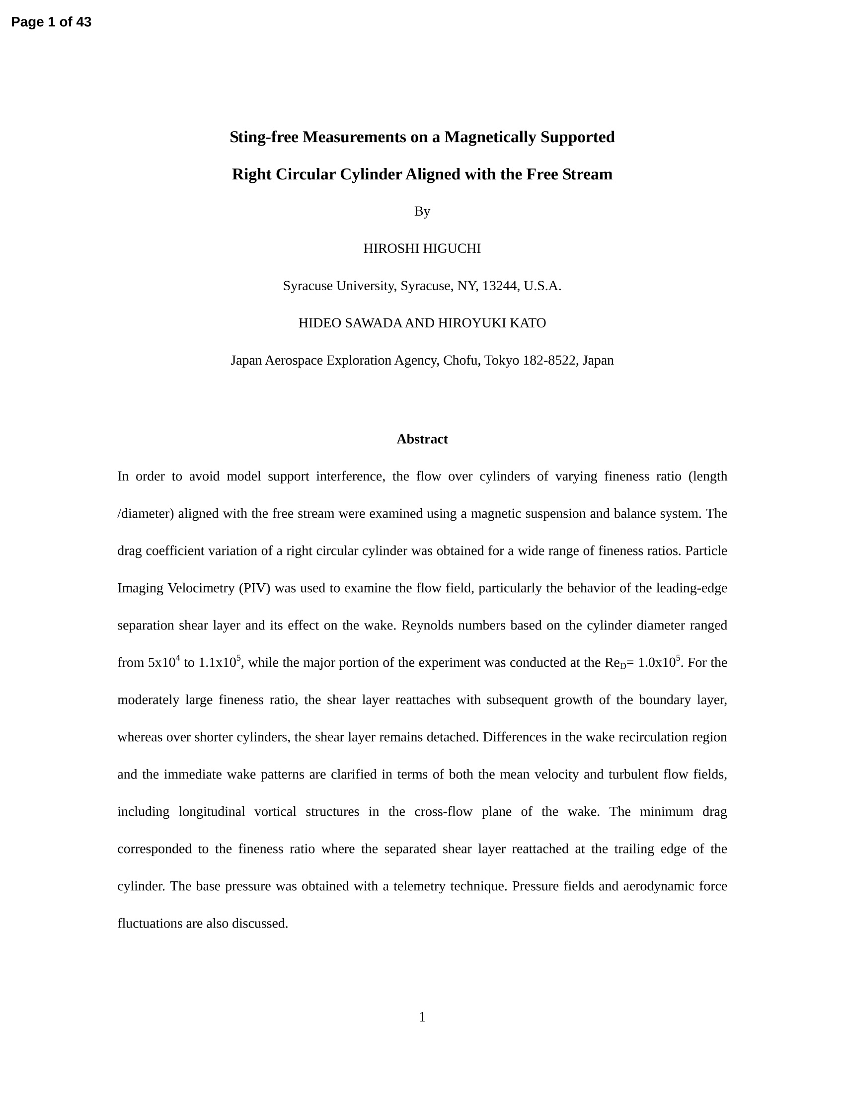
In order to avoid model support interference, the flow over cylinders of varying fineness ratio (length
/diameter) aligned with the free stream were examined using a magnetic suspension and balance system. The
drag coefficient variation of a right circular cylinder was obtained for a wide range of fineness ratios. Particle
Imaging Velocimetry (PIV) was used to examine the flow field, particularly the behavior of the leading-edge
separation shear layer and its effect on the wake. Reynolds numbers based on the cylinder diameter ranged
from 5x10⁴ to 1.1x10⁵, while the major portion of the experiment was conducted at the ReD= 1.0x10⁵. For the
moderately large fineness ratio, the shear layer reattaches with subsequent growth of the boundary layer,
whereas over shorter cylinders, the shear layer remains detached. Differences in the wake recirculation region
and the immediate wake patterns are clarified in terms of both the mean velocity and turbulent flow fields,
including longitudinal vortical structures in the cross-flow plane of the wake. The minimum drag
corresponded to the fineness ratio where the separated shear layer reattached at the trailing edge of the
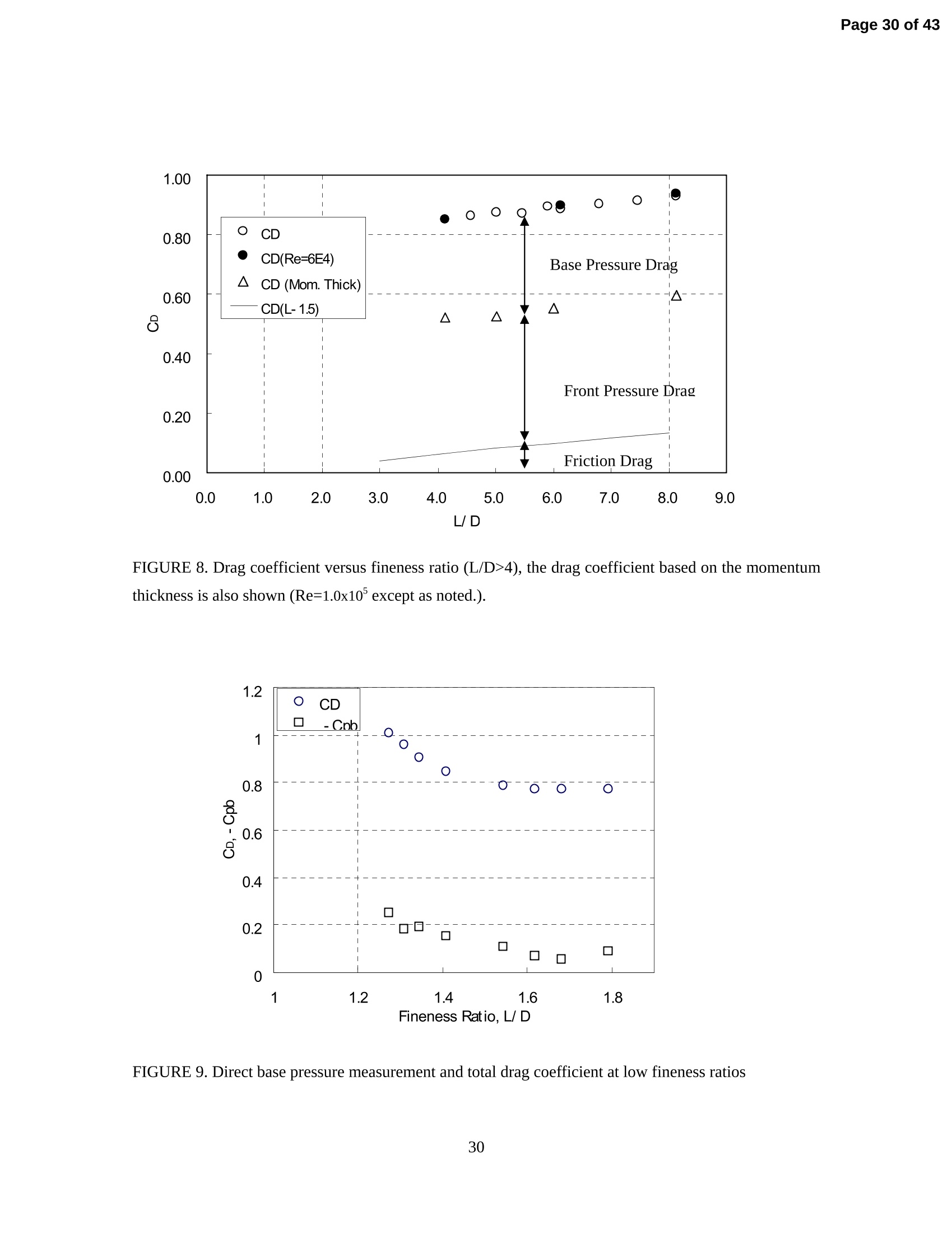
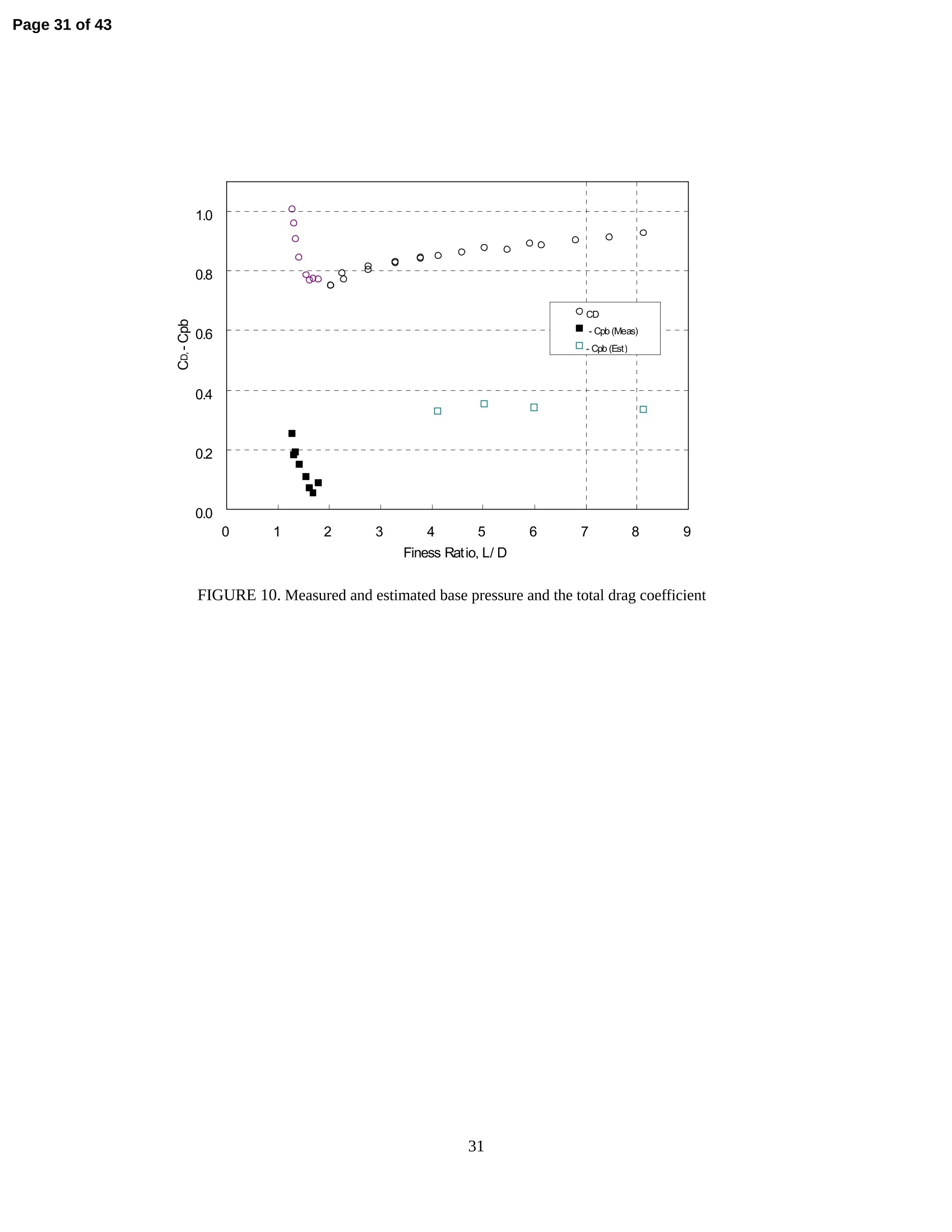
cylinder. The base pressure was obtained with a telemetry technique. Pressure fields and aerodynamic force
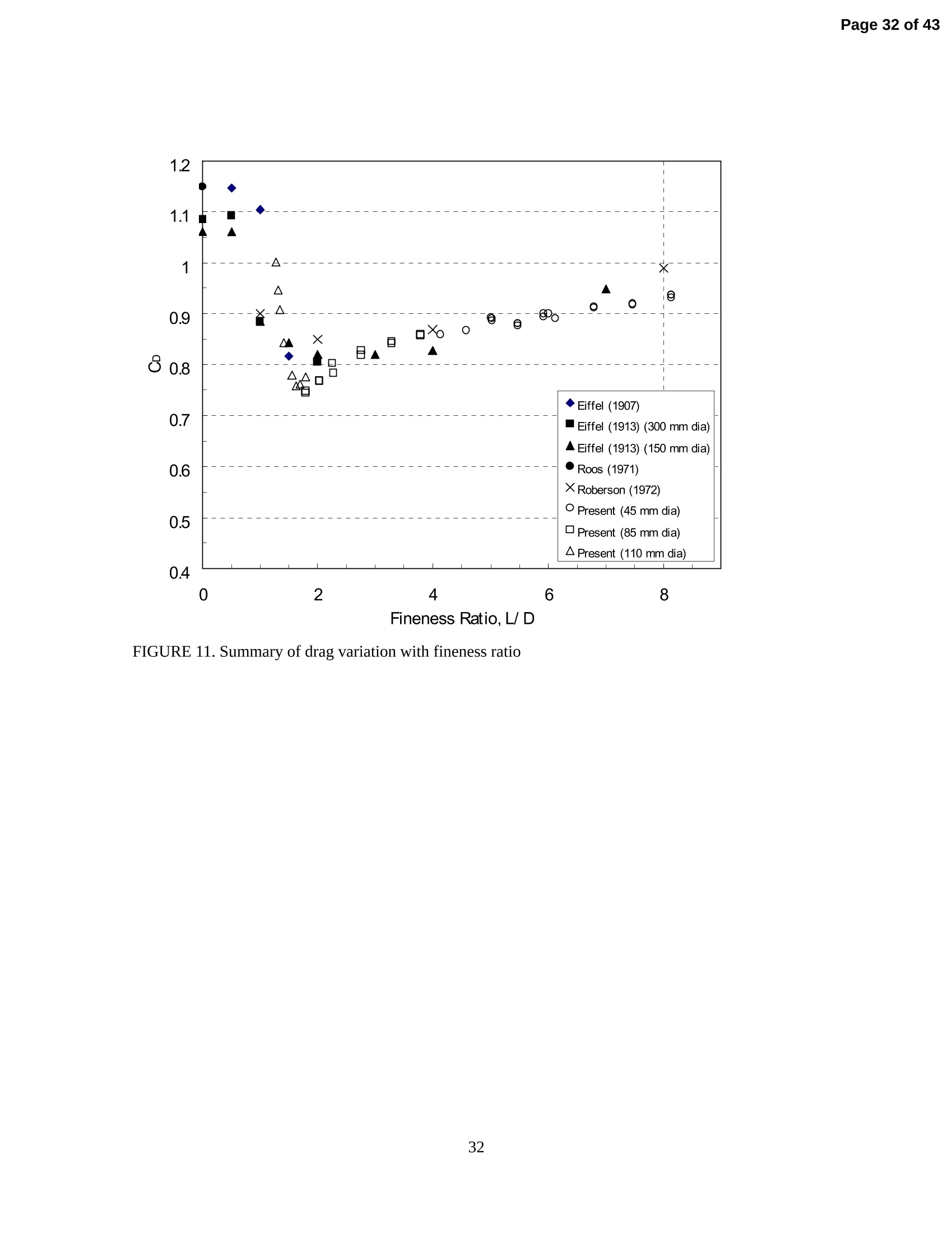
fluctuations are also discussed.
方案详情

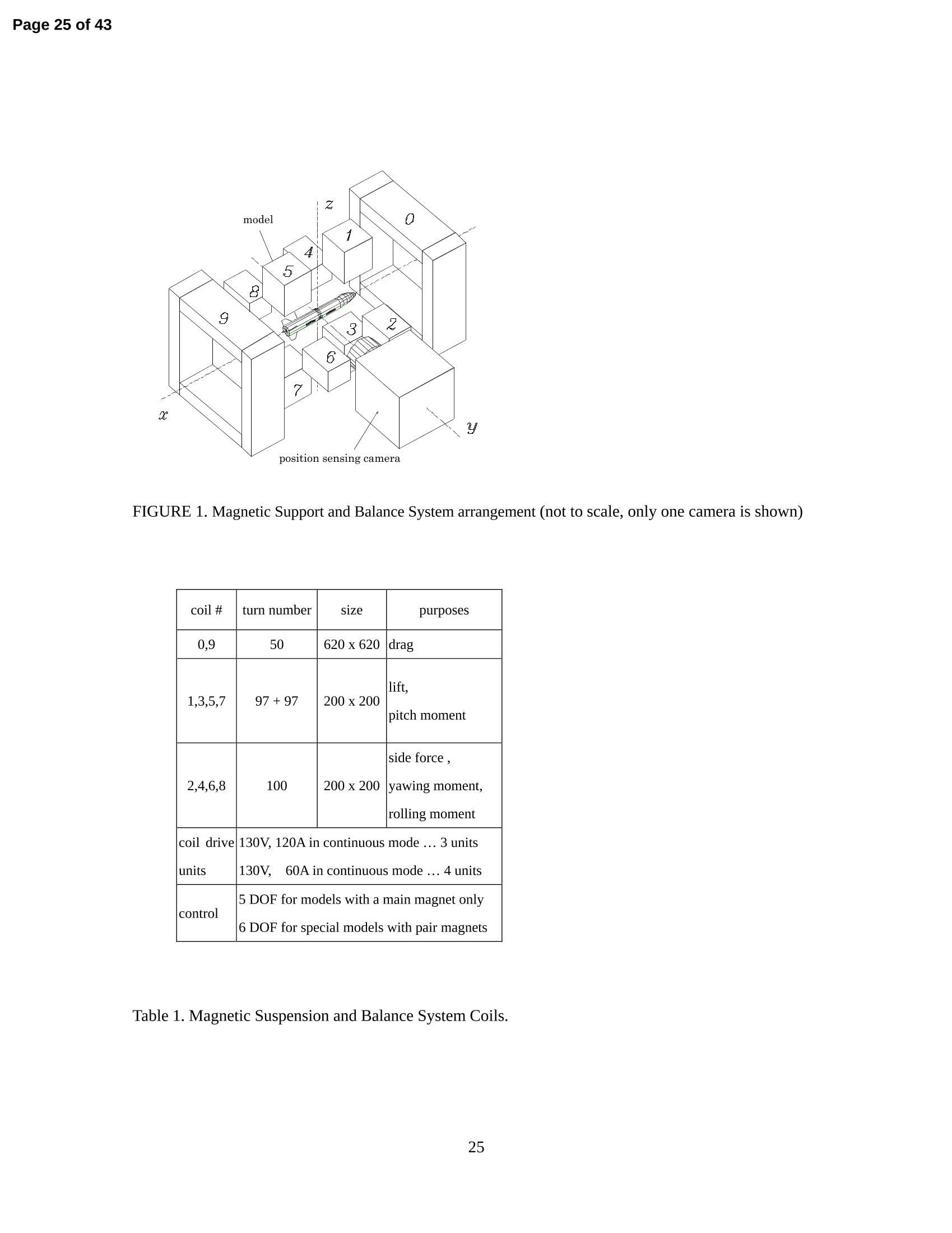
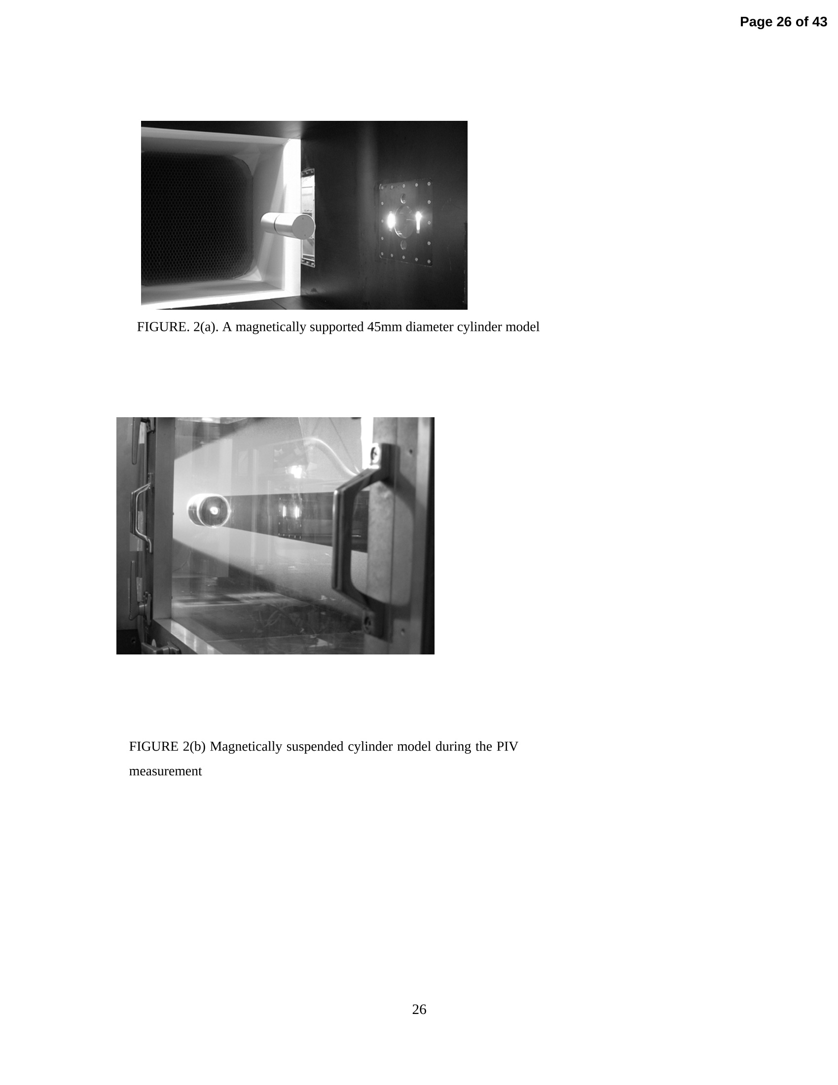
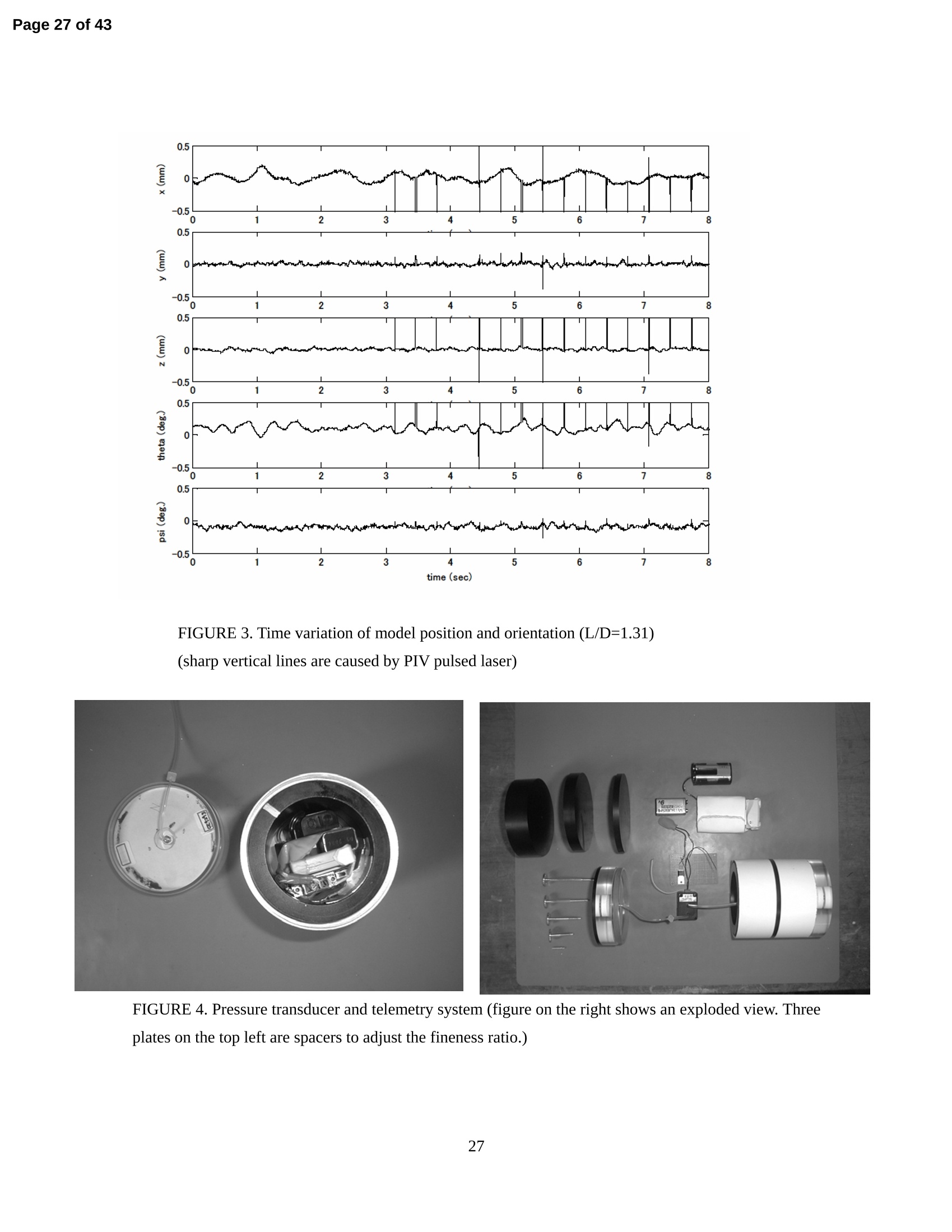
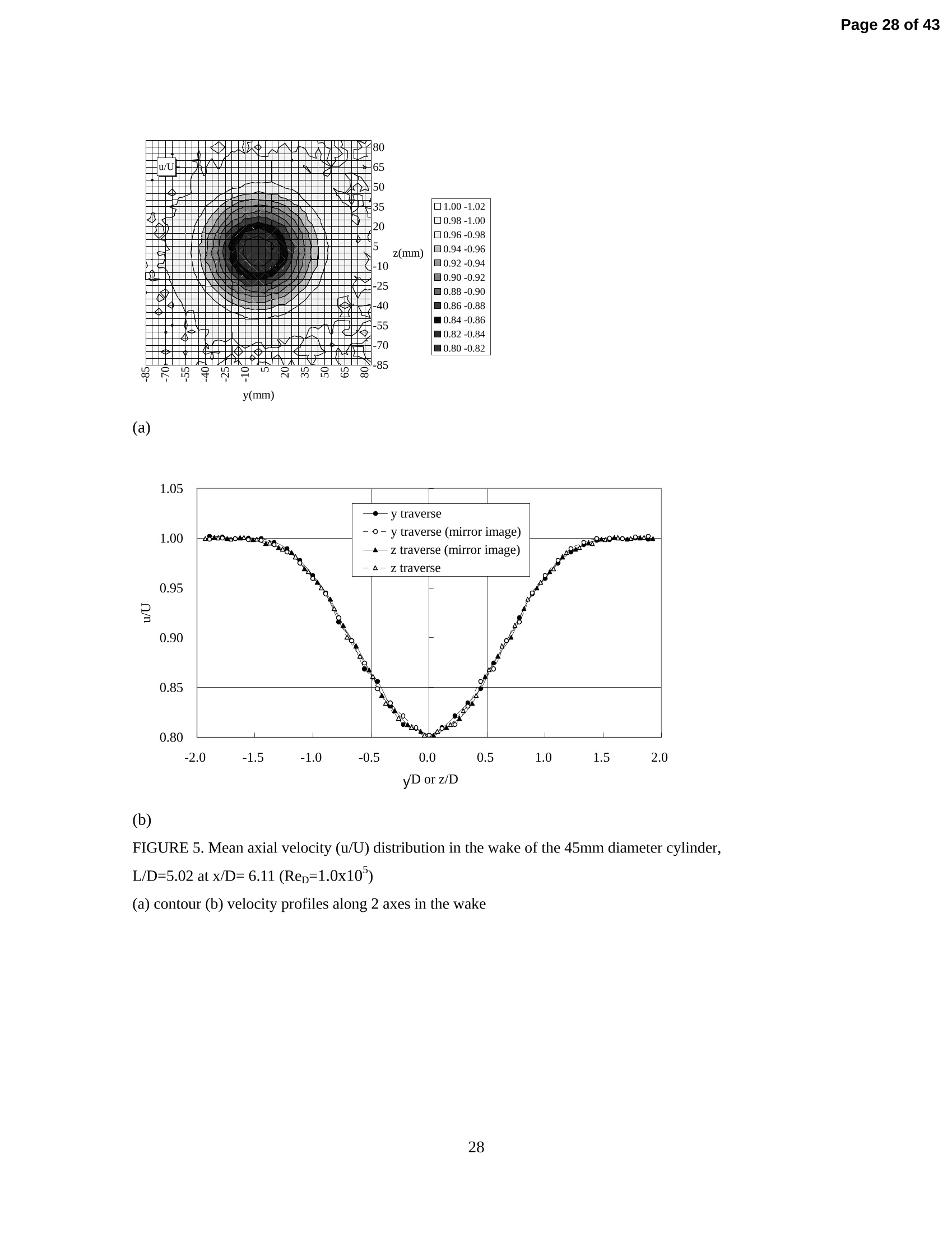
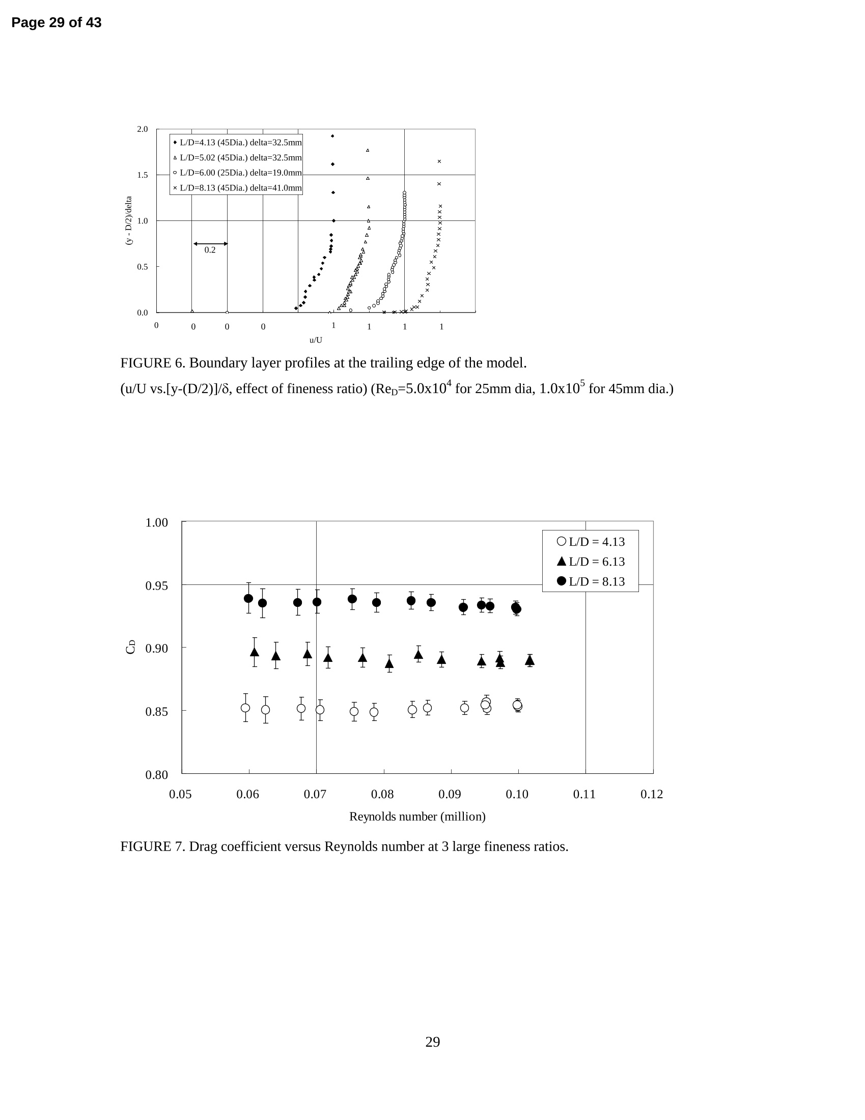
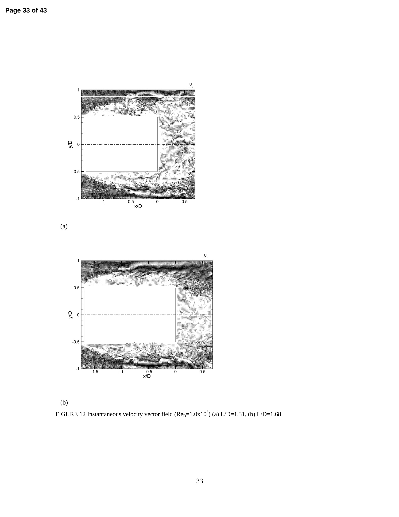
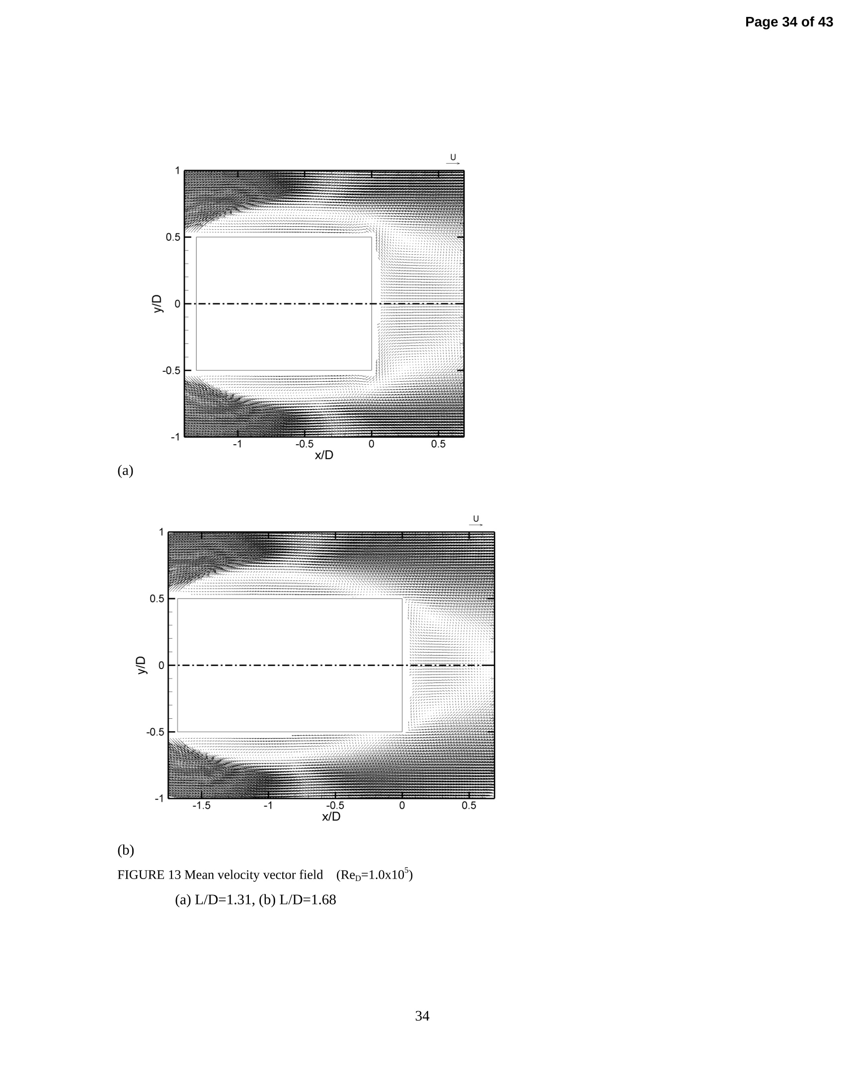
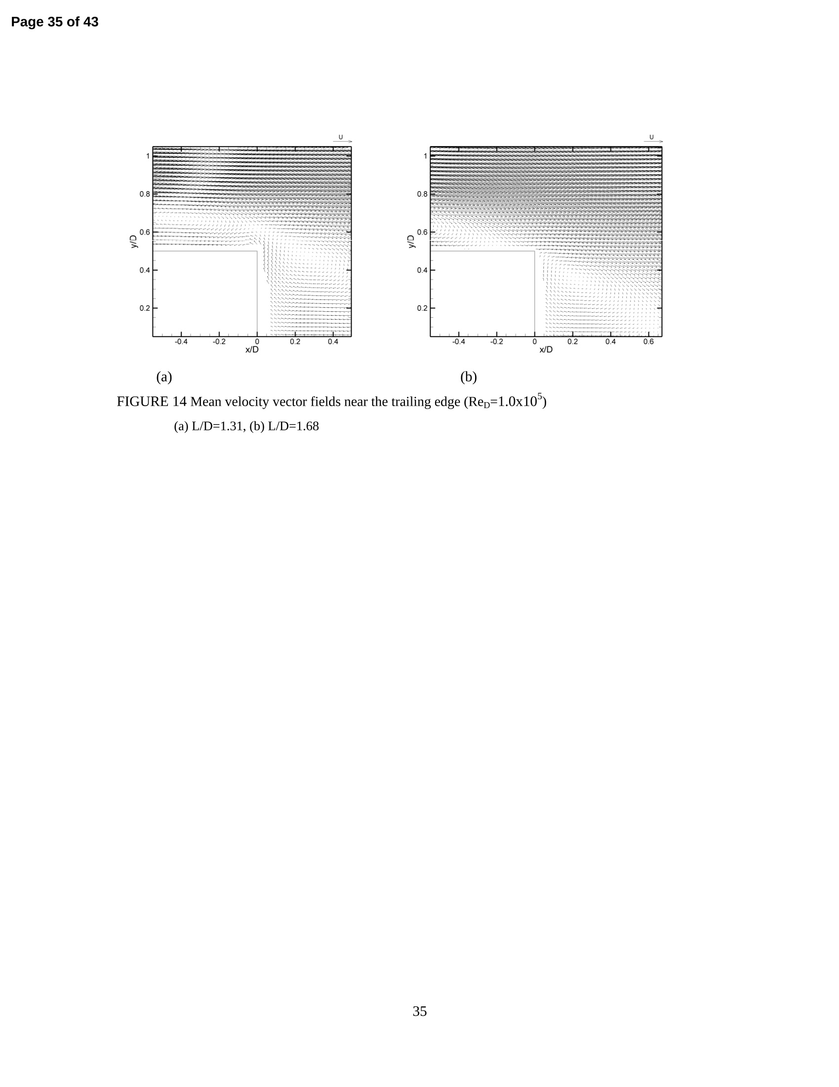
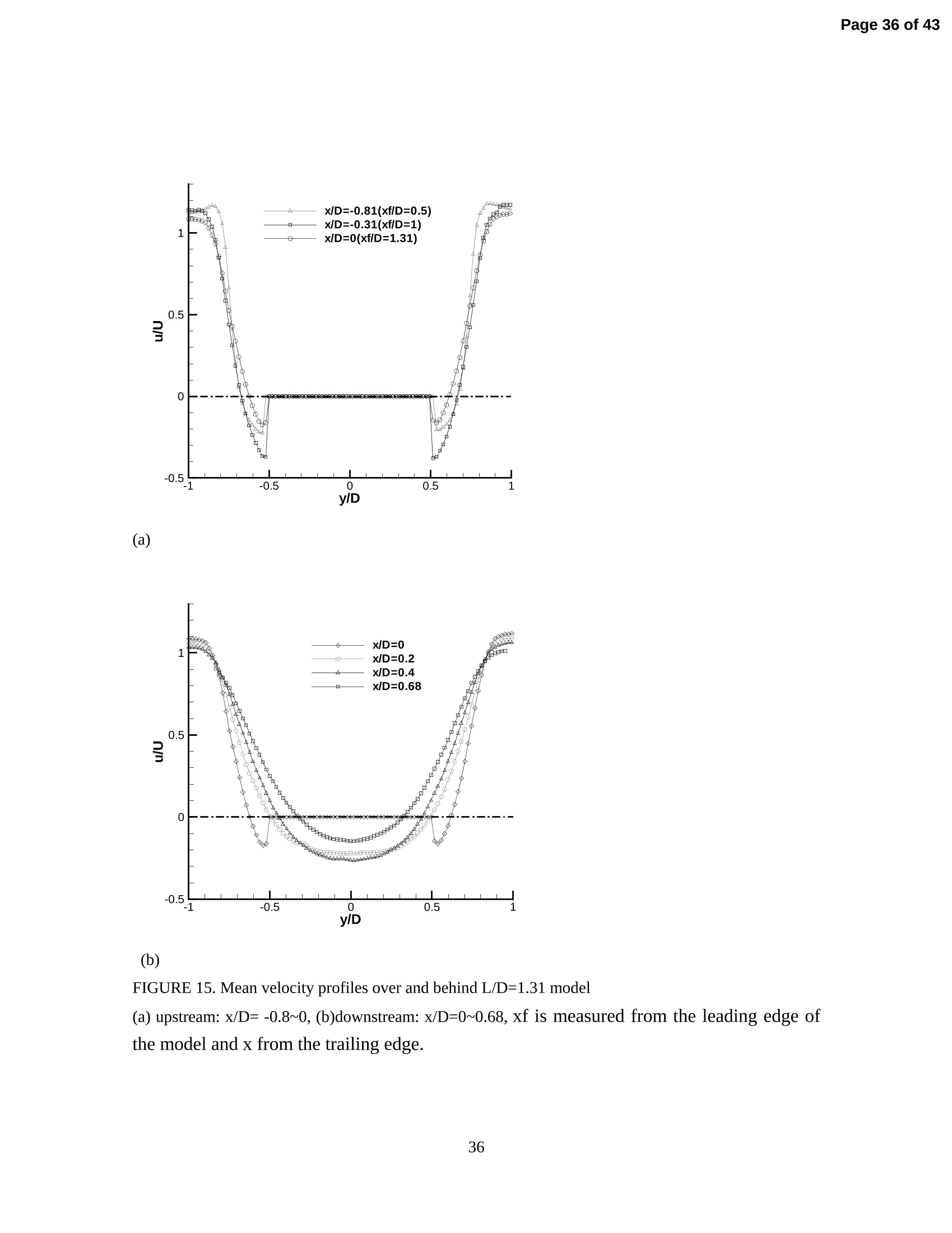
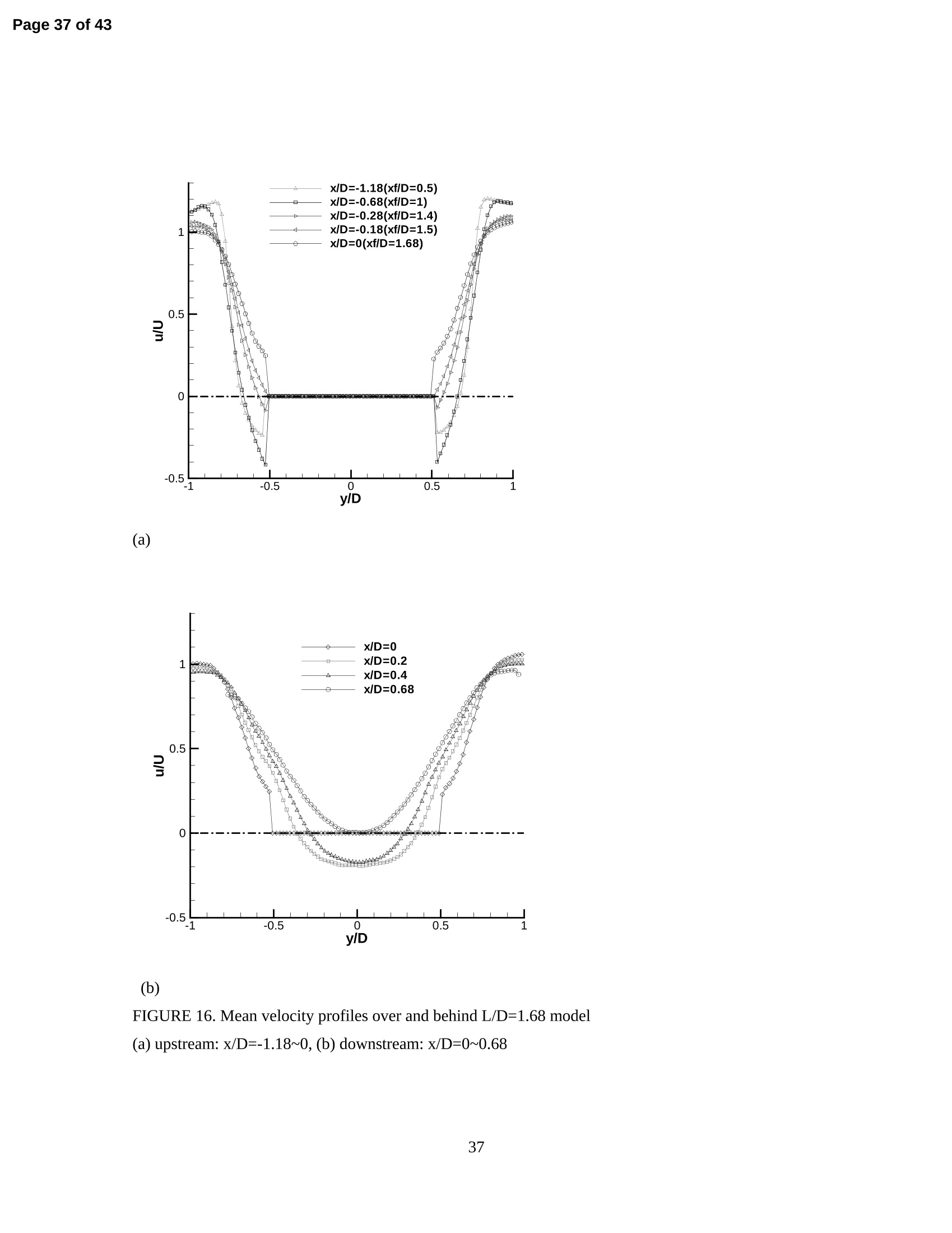
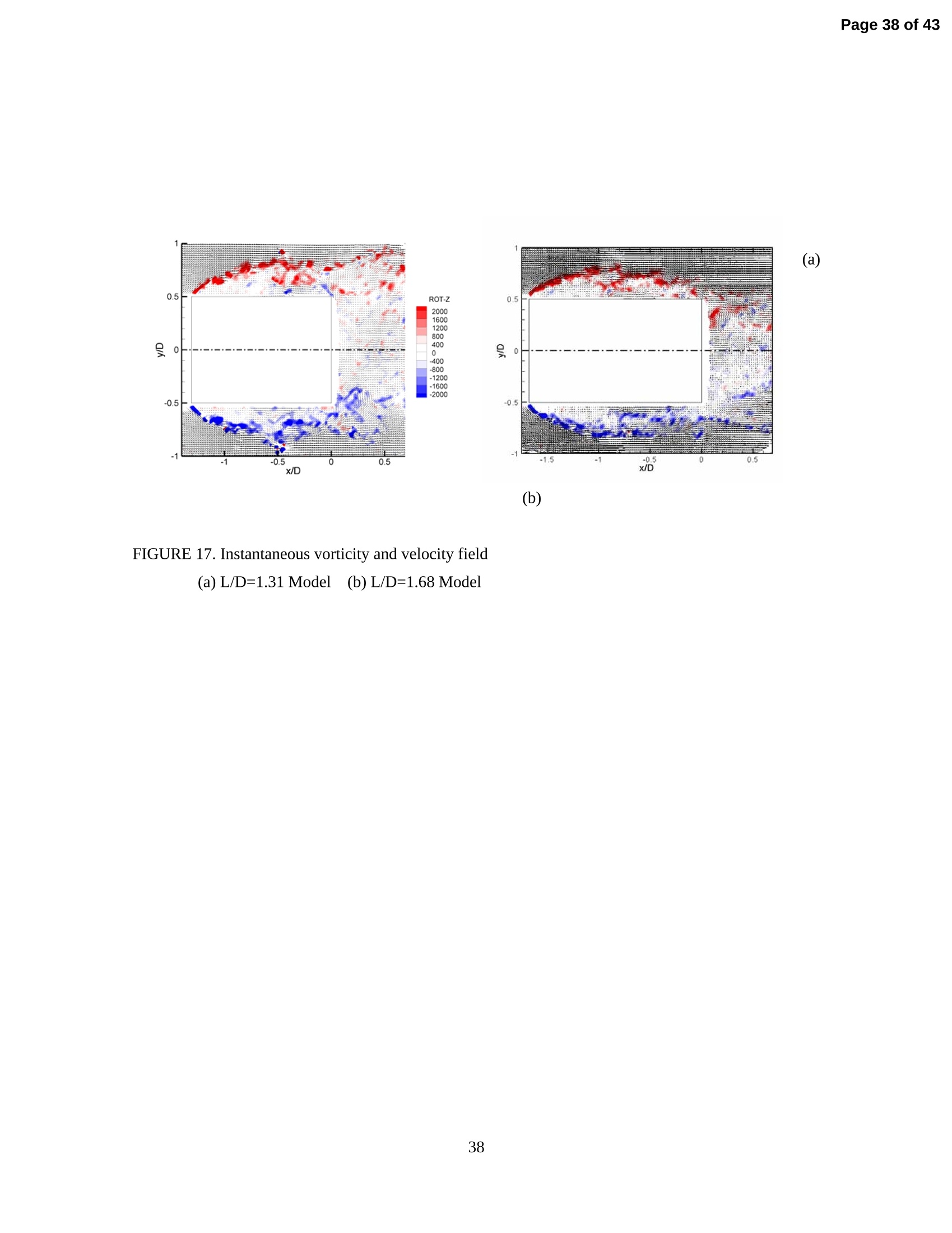
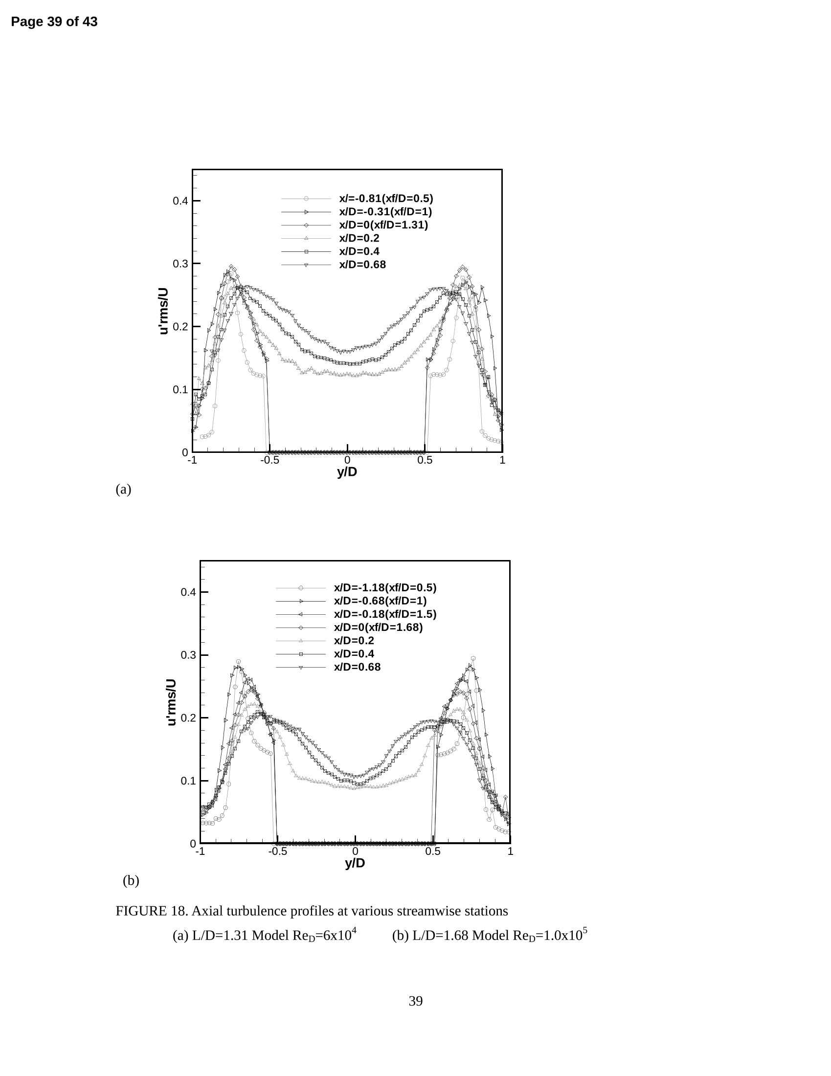
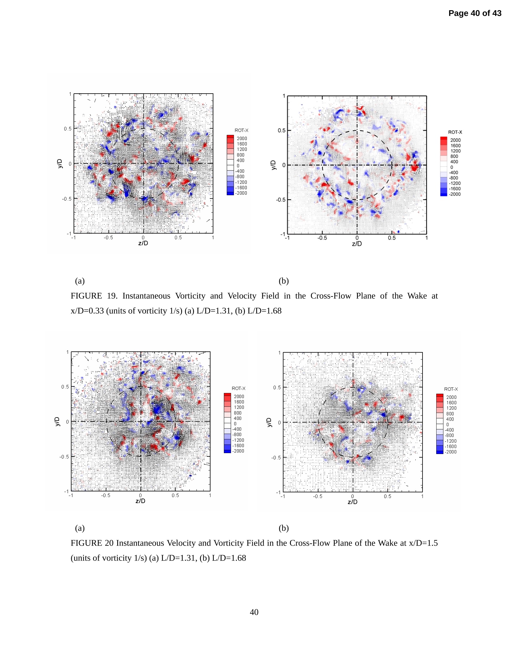
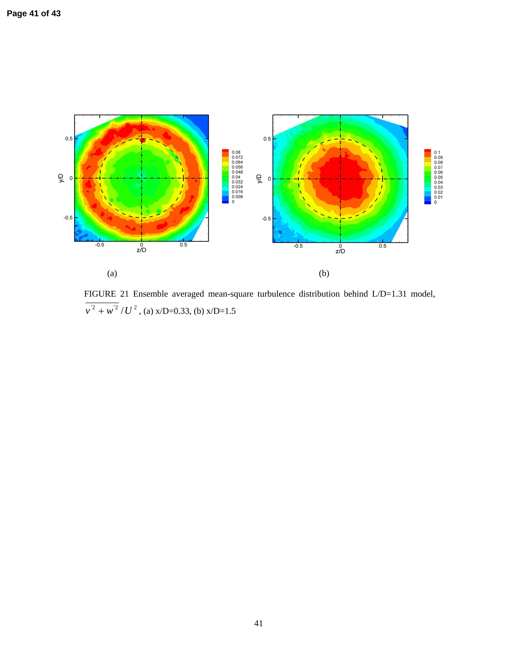
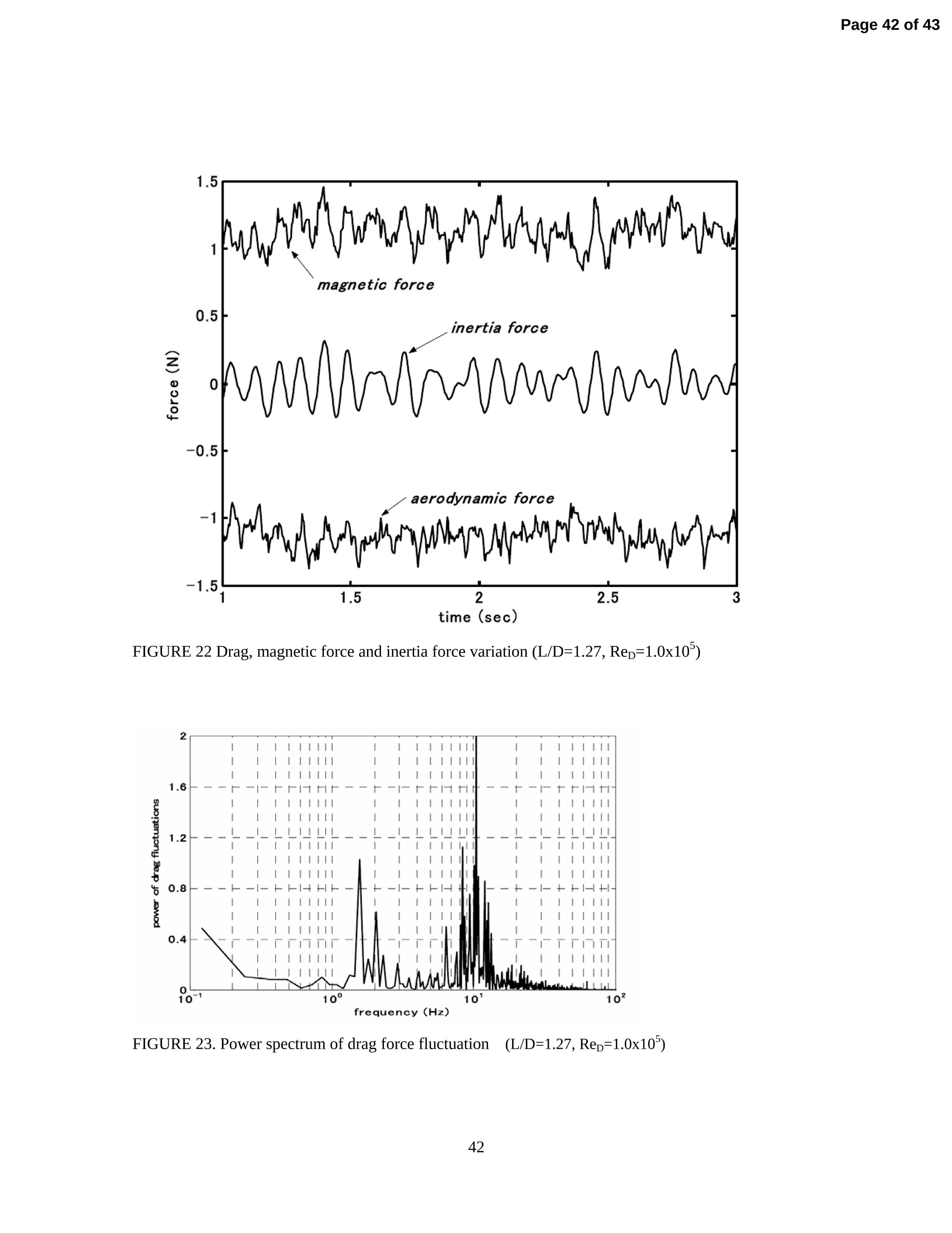
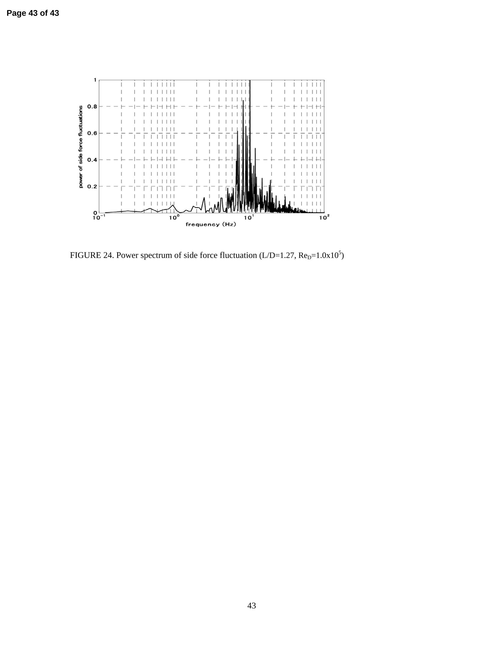
Page 1 of 43 Sting-free Measurements on a Magnetically Supported Right CircularCylinder Aligned with the Free Stream Journal: Journal of Fluid Mechanics Manuscript ID: JFM-06-S-0619.R3 mss type: Standard Date Submitted by the Author: 24-Aug-2007 Complete List of Authors: Higuchi, Hiroshi; Syracuse University, Mechanical & Aerospace Eng.Sawada, Hideo; Japan Aerospace Exploration Agency, Institute ofSpace Technology and Aeronautics Kato, Hiroyuki; Japan Aerospace Exploration Agency, Institute ofSpace Technology and Aeronautics Keyword: Separated flows <; Wakes/Jets, Flow@structure interactions <;Aerodynamics,Interactions &It; Vortex Flows Sting-free Measurements on a Magnetically SupportedRight Circular Cylinder Aligned with the Free StreamBy HIROSHI HIGUCHI Syracuse University, Syracuse, NY, 13244, U.S.A.HIDEO SAWADA AND HIROYUKI KATO Japan Aerospace Exploration Agency, Chofu, Tokyo 182-8522, Japan Abstract In order to avoid model support interference, the flow over cylinders of varying fineness ratio (length/diameter) aligned with the free stream were examined using a magnetic suspension and balance system. Thedrag coefficient variation of a right circular cylinder was obtained for a wide range of fineness ratios. ParticleImaging Velocimetry (PIV) was used to examine the flow field, particularly the behavior of the leading-edgeseparation shear layer and its effect on the wake. Reynolds numbers based on the cylinder diameter rangedfrom 5x10" to 1.1x10, while the major portion of the experiment was conducted at the Rep=1.0x10. For themoderately large fineness ratio, the shear layer reattaches with subsequent growth of the boundary layer,whereas over shorter cylinders, the shear layer remains detached.Differences in the wake recirculation regionand the immediate wake patterns are clarified in terms of both the mean velocity and turbulent flow fields,including longitudinal vortical structures in the cross-flow plane of the wake. The minimum dragcorresponded to the fineness ratio where the separated shear layer reattached at the trailing edge of thecylinder. The base pressure was obtained with a telemetry technique. Pressure fields and aerodynamic forcefluctuations are also discussed. 1. Introduction Axial flow along a circular cylinder represents a canonical configuration that is applicable to aircraftfuselages, missiles, road vehicles, etc. The drag coefficient of the cylinder aligned with the flow is listed invarious handbooks and textbooks (see, e.g., Blevins 1984, Crowe et al. 2005). Blevins quotes Nakaguchi(1978) but the original source dates back to Hoerner (1958) who in turn quoted Eiffel's experiments (1907,1913). The Eiffel tower was used in the 1907 experiment where various models were dropped along a guidecable. Eiffel repeated the experiment in a low-speed wind tunnel in 1913. While some additional dragmeasurements were conducted by Roberson et al. (1972), no modern systematic measurement is available forthis configuration and the classical data may be subject to possible interference from sting-mounted dragbalances. In this investigation, we decided to re-examine the flow over this very well-defined geometry, withthe key parameters being the length-to-diameter ratio (fineness ratio) and the Reynolds number. Here the termfineness ratio was adopted, see Hoerner (1958), though other terms such as slenderness ratio or aspect ratiomay be as applicable. The resulting flow field is complicated and involves a separated shear layer from thesharp leading edges that may or may not re-attach at a given fineness ratio, ultimately affecting the subsequentboundary layer development. At the end of the cylinder, the boundary layer separates from the trailing edgeand is followed by a recirculation region and three-dimensional wake structure. Since the flows about the front face, in the boundary layer and in the wake of the axisymmetric body are allcritical to accurately determining the drag coefficient, the traditional model support poses certain difficulties.In order to avoid any interference from model sting or other support, the present experiment utilized theMagnetic Suspension and Balance System at the Institute of Space Technology and Aeronautics, Japan AerospaceExploration Agency. Precise model alignment is easily implemented, and the instantaneous forces and momentacting on the entire body are directly measured as a part of feed-back control system. This approach avoidsthe introduction of unnecessary interference or flow disturbance due to a conventional force balance. A new, more definitive data set of drag coefficients over a wide range of fineness ratio has been obtained, and theeffect of the shear layer reattachment has been investigated in further detail with the flow field measurements.The phenomenon of flow separation from the shoulder of the cylinder and its reattachment was studied byKiya et al.(1991)who found a cellular structure in the reattachment region. Their models were supported fromdownstream. In a typical laboratory setup, however, due to the necessity of supporting the model with wires ora sting, the leading edge shear layer and the wake, as well as the interaction between them, are difficult toobserve simultaneously. In our own recent study using a water channel and the PIV system, the flow structures of the separating andreattaching shear layer and of the wake behind a sting-mounted cylinder were examined (Higuchi et al. 2006).The wake of a supporting strut was found to influence the cross sectional mean velocity profile downstream,and a disturbance from upstream was detectable in the instantaneous velocity field. A snapshot ProperOrthogonal Decomposition revealed two symmetrical pairs of counter-rotating longitudinal vortex structureswhich were deemed to be a part of the intrinsic flow field, though the first mode clearly showed the supportinterference. Therefore, in order to avoid any such interference of the support on flow field measurements, the presentstudy employed PIV in conjunction with a magnetically suspended model. There have been studies onmagnetically supported models in the past (e.g., Judd et al.1971), but the experiments were restricted to meandrag force measurements because the limited model size and instrumentation techniques were not appropriatefor this type of unsteady separated flow. Here, modern digital PIV was incorporated for velocity fieldmeasurement without interference from the model support and the base pressure was measured using atelemetry system. 2. Description of Experiment and Set-Up 2.1. Magnetic model suspension, force balance and wind tunnel The experiment was conducted using the Magnetic Suspension and Balance System at the Institute of SpaceTechnology and Aeronautics, Japan Aerospace Exploration Agency (JAXA). The system was developed by Sawadaand his group (Sawada and Kunimasu, 2001). Figure 1 shows schematically the coil (or electromagnet)arrangement used in the system, and the specifications of the individual coils are listed in Table 1. Here, thecolloquial term, coil, is used as it appeared in the reference above. This particular figure is for a smallerprototype, but the arrangement is clearly shown. Five pairs of coils provide necessary control of the model inall directions. The currents to individual coils provide instantaneous drag, lift, side force, and pitching andyawing moments. The model position and attitude were monitoredl by two CCD cameras orientedorthogonally to each other and controlled at a 248Hz feedback frequency. Two colors and filters were used toseparate reflected light in two directions. The balance system was installed in the subsonic wind tunnel with a60cm x 60cm test section. Compared to earlier systems reported in the past (Judd et al, 1971), the size of thepresent magnetic suspension and balance system affords adequate spatial resolution for accurate flow fieldmeasurements. The available flow speed ranged from 10 to 35 m/s with a free stream turbulence level lessthan 0.08%. The magnet current was calibrated against a known force applied through pulleys and weights foreach model and had a repeatability within 0.2% (Sawada, et al, 2004). Further detail of the MagneticSuspension and Balance System and the wind tunnel can be found in Sawada et al (2001). 2.2. Test models Each model was made from aluminum alloy and was housed a rod-shaped or annular permanent magnetalong the centerline. Figure 2 illustrates the cylindrical models supported magnetically in the test section. Inaddition to the model edges, the sensing cameras use a vertical stripe, located in the middle, to detect the model position and attitude. In order to provide a wide range of fineness ratios, models with differentdiameters were used. One had 45mm diameter (see figure 2a) and shared the same center section enclosingthe permanent magnet. By changing the end caps of different lengths, nine fineness ratios between 4.13 and8.13 were achieved. A second model had a diameter of 85mm and the third 110mm. These larger diametermodels provided a fineness ratio down to 1.272. An additional model of 25mm diameter and fineness ratio of6 was also used. The Reynolds number based on the diameter ranged from 5x10 to 10. Figure 2(b) showsthe 110mm diameter model suspended in the test section illuminated by the pulsed laser sheet during the PIVmeasurement. For force measurements, as well as some initial flow measurements using conventional hotwire probe andpressure probes, the test models ranged in diameter from 25mm to 110 mm to provide a wide range offineness ratios. In the present velocity field measurement with the PIV system described in the next section,the diameter of the model was fixed at 110mm and two lengths were chosen to provide L/D=1.31 and 1.68.The position was controlled within ±0.2mm in any direction and the yaw and pitch angles of the model wereheld constant within ±0.1degree. Typical instantaneous control current and the model position are shown infigure 3. Sharp pulses in the figures are due to the laser light sheet for the PIV (see figure 2(b)). The basepressure measurement was also conducted with the 110mm diameter model. Position sensing for these shortmodels needed special attention as described in Sawada et al. (2001). The optical sensing of the modelposition was not affected by the pulsed laser light sheet applied to measure the velocity field. Time historiesof the position and the coil currents will be discussed in the results section below. 2.3. Particle Image Velocimetry (PIV) system set up A 2-Component PIV system developed for the JAXA wind tunnels (Watanabe and Kato, 2003) wasemployed for the present experiment. The laser is a two-cavity double-pulse Nd:YAG (Quantel, Twins CFR 200) with maximum pulse energy of 200 mJ/pulse at a repetition rate of 15 Hz. The cross-correlation camera(LaVision, Imager Pro Plus 4M) has a 14-bit monochrome CCD image sensor with 2048 x 2048 pixels. Whilethe original framing rate of the camera is about 15 Hz, two-component velocity vector maps in the 2-D PIVmeasurement are obtained at around 1.5 or3 Hz, being limited by the data transfer rate to the storage system.The timing between the image acquisition by the CCD camera and the laser pulse was synchronized by aprogrammable timing unit. Time separation At was set between 25 and 95 us according to the flow speed. Oildroplets with a diameter of around 1um were used as the seed particles. In the PIV measurement, the wholeflow path of the wind tunnel was seeded by a seeding generator (LG-500) developed by the GermanAerospace Center (DLR), with five Laskin nozzles and an impactor plate for generating small seed particlesof uniform size. Two PIV setups were used in these measurements. In one setup, the laser light sheet waslocated perpendicular to the free stream. In another setup, the laser light sheet was located parallel to the freestream, including the model center axis (See figure 2b). A small mirror was installed into the wind tunneldiffuser due to the limitation of optical access, and a small optical window was created on the diffuser wall forthis experiment. In the case of measurement perpendicular to the free stream, the camera was located outsideof the diffuser and the seeding image was acquired at right angles to the laser light sheet through the mirror. Incase of the measurement plane parallel to the free stream, the laser light sheet was directed upstream by themirror, and the camera was located along the side wall of the test section. The size of the PIV measurementregion was about 250mm x 250mm in the both setups.Commercial PIV software (LaVision, DaVisFlowMaster) for acquisition and post processing of the images ran on a PC with 3.06GHz dual Xeonprocessors. Typically 2000 pairs of images were captured per run and were stored onto a 6 TB ArrayMasStorL-HP RAID System. Pairs of particle images acquired by the CCD camera were analyzed by means of the Fast FourierTransform (FFT)-based cross correlation technique in the PIV software, resulting in two-component vector maps. In order to achieve sub-pixel accuracy in the vector analysis, Gaussian curve fitting was adopted as thepeak search algorithm. The vectors are calculated with 50 % overlap between adjacent interrogation regions.Erroneous vectors were only omitted through a peak ratio filter without interpolation for the omitted vectors.Instantaneous data at an identical test condition are ensemble averaged, yielding mean vector maps andprofiles. All the instantaneous velocity data are saved for present and future analyses. 2.4 Base Pressure Measurement Since no support strut or sting is available to transmit pressure measurements or electrical signals, atelemetric system was employed to measure the base pressure on the magnetically suspended models. Theelectronic pressure transducer, A/D converter and the radio transmitter, as well as a battery to power the unit,were all housed within the test model as shown in figure 4 (Sawada et al. 2005). An annular permanentmagnet was used to accommodate the instrumentation within the model. The system was speciallyco-developed by JAXA and NEC Engineering and allows 4 channel simultaneous 12.5 kHz sampling and12-bit resolution A/D conversion. The digital data were transmitted through a bi-directional wireless LANmethod. In addition, it had a 4-bit digital signal source that could be externally controlled. A differentialpressure gage of 500 Pa full scale was housed within the model powered by a 9 volt battery. Two 0.5mmdiameter pressure taps were placed on the cylinder axis at the front and back faces of the model. Figure 4bshows the individual components in the assembly. Due to space limitations, the device was only incorporatedinto the 110 mm diameter models, i.e. the low fineness ratio range. 3. Results and discussion 3.1. Initial wake survey behind the magnetically supported cylinder Preliminary velocity measurements relied on a more conventional total head probe and a hot-wire probe on2-axis traversing system and the results are limited to regions where the instrumentation was suitable. Themean velocity distribution measured with a pressure probe behind the L/D=5.02 model is presented in acontour map. as well as in both vertical (z) and horizontal (y) directions, see figure 5. The origin of theco-ordinate system is located at the trailing edge of the model, with the x-component being in the streamwisedirection. The mean velocity components (u,v,w) correspond to the (x,y,z) directions, respectively, and U isthe free stream velocity. The figure demonstrates the excellent flow axisymmetry achieved here, clearlybenefiting from the absence of the model support in the present system. A comparison of the results from PIVmeasurements behind a sting-mounted model presented by Higuchi et al (2006) and those from PIVmeasurements with the current magnetic suspension system will be discussed below. The boundary layer profiles at the trailing edge were measured with a hot wire probe for various finenessratios and the mean velocity profiles, normalized by the boundary layer thickness, are shown in figure 6. TheReynolds number was 5x10* for the 25mm cylinder and 1x10’for the 45mm cylinder. Ota (1975) investigatedthe boundary layer over a sting-mounted sharp-edged cylinder. His velocity profiles, obtained at x/D=3.1, 5.1,and 7.1 from the leading edge, are consistent with the present data at the trailing edge (L/D=4.13-8.13). Ota’sexperiment corresponded to Rep=5.62x10 and his measurement showed a separation bubble extending fromthe leading edge and ending with flow reattachment approximately 1.5-1.6 diameters downstream. The meanvelocity profiles beyond the reattachment zone indicated a developing turbulent boundary layer. Turbulenceintensity profiles are also in general agreement between the two hot-wire measurements, though the presentdata are somewhat greater. The power spectral density in the immediate wake and shear layers showed the distribution typical of a turbulent boundary layer devoid of any spectral peak. However, at x/D=4, a spectralpeak was evident at Strouhal number St=fD/U=0.185, indicative of a helical mode wake oscillation. 3.2. Force and base pressure measurements As stated earlier, the coil currents needed to hold the model in place provided the lift, drag, and sideforce, as well as the pitching and yawing moments. The magnetic balance was calibrated against the knownweight for each model. The blockage ratio of the model varied between 0.44% and 2.64% depending on themodel diameter in use. While the blockage is small, the results shown incorporate the standard blockagecorrection by Pankhurst and Holder (1952), which was also employed by Judd et al. (1971). The correctionreduces the drag coefficient up to 2-3% for the largest model. Since the instantaneous currents to individualcoils were recorded, force-time histories can be analyzed as shown in the later section once the mass andmoment of inertia of each model are known, but here only the time averaged force has been extracted for allcases. As expected, pitching and yawing moments as well as lift and side forces averaged to be zero and thusonly the drag force will be presented and discussed. Figure 7 shows the measured drag coefficients for the three large fineness ratios over the range ofReynolds number approximately between 6x10 and 10. The experimental uncertainty is also noted. TheReynolds number dependency as estimated by the empirical skin friction drag for the turbulent boundary layeris not as clearly manifested in the measurement, but the expected amount of variation within this Reynoldsnumber range is of the same order as the uncertainty of measurement. For the separation dominated flow fieldover the models between L/D=1.27 and 1.79, the Reynolds number dependency on the drag coefficient wasnegligible. On the other hand, the fineness ratio had a clear influence on the total drag coefficient, as shown atthe top of figure 8 for Re=10. The measured drag data at Re=6x10"are also included. In order to estimate theindividual contributions to the total drag, figure 8 shows the momentum loss based on the boundary layer measurement shown in figure 6, and the estimated skin friction drag as well as the total drag. The skin frictionwas estimated from the empirical power-law formula for a flat plate turbulent boundary layer (see e.g.,Schlichting 1968). The skin friction drag varies as the 1/5h power of Reynolds number based on the length,and thus is proportional to the product of Re-1/5 and (L/D)4/5. Here, the separated flow at the front corner isconsidered to attach at 1.5 diameters downstream (Higuchi et al 2006) and thus the effective length has beenreduced accordingly. A similar trend is seen among all three curves. As indicated in the figure, the differencebetween top two lines is, in effect, the base pressure, and that between the bottom two lines corresponds to thepressure drag on the front face. In both cases, they are nearly independent of the fineness ratio. The base pressure was measured for short cylinders between L/D=1.27 and 1.79 concurrently with the totaldrag measurement and the results are given in figure 9 for Re=10. The base pressure behind L/D=1.27 and1.35 cylinders increased slightly with Reynolds number within the range 5x10~10, while the model withL/D=1.79 exhibited almost constant base pressure within this range. The leading edge shear layer presumablyremained detached at the lower fineness ratio, so the Reynolds number dependence may be attributable to thechange in radial width of the separated shear layer region and wake vortex roll-up. In figure 9, it can be seenthat for cylinders of small fineness ratio, the variation in total drag is due to changes in base pressure since thefront pressure is expected to be unchanged amongst the models and the separated shear layer remainsdetached (presuming the reverse wall shear stress is small). Both the measured base drag at low finenessratios and the estimated base drag in figure 9 are plotted together in figure 10 to contrast the variationsbetween the short and long cylinders. The base pressure of long cylinder is nearly constant whereas the basepressure depends strongly on the fineness ratio for the short cylinder. Finally, all of the present drag measurements are summarized in figure 11. All of our data shown in thefigure are for the Rep=10. The uncertainty in the drag coefficient is about ±0.5-2% (larger uncertainty forL/D<2).) Previous and historical data are also included. The first drop experiment by Eiffel (1907) was at a Reynolds number estimated to be between 5.5x10and 1.1x10. The second set of Eiffel data (1913) wascollected in a wind tunnel with the models cable-mounted in the test section. The experiment predates listingof Reynolds number but is estimated to be nominally in the 1x10~2x10°range. Apparently Hoerner (1958)used Eiffel’s second data set (not as listed in his book) and subtracted the estimated skin friction and presentedthe data in figure 21, Chapter 3 of his book. As mentioned before, these values have been quoted for decadesin many articles, reference books and textbooks, not necessarily after critical evaluation. Roos and Willmarth(1971) measured the drag coefficients of sphere and disk over a very wide range of the Reynolds number, andtheir result of the disk as a limiting case of L/D=0 is shown for Re=6.04x10",the highest Reynolds numberthey reported. Roberson et al. (1972) carried out new wind tunnel measurements on cylinders to study theeffect of the high free stream turbulence, and the data in their data in figure 11 correspond to the Reynoldsnumber of 4x10 without grid turbulence imposed. There is significant scatter in the prior data for the very low L/D range. It is known that the drag coefficientof a two-dimensional rectangular cylinder reaches the maximum value when the fineness51ratio isapproximately 0.6 due to the interaction between the wake vortices and the model base (Bearman andTrueman, 1972, Park and Higuchi 1989, Ohya 1994). Helical vortex formation downstream of theaximmetric model is expected to produce substantially different interactions with the base planeUnfortunately, as currently configured, the present magnetic suspension system did not allow experiments atextremely low L/D ratios due to the housing of the magnet and model alignment. This issue will be addressedin future investigations. Nevertheless, the present series of experiments is expected to provide more accurateresults for the drag coefficient and to yield an improved understanding as to how the drag and the flowfieldvary over a wide range of fineness ratio. 3.3. Flowfield measurement 3.3.1. Velocity field In the previous water channel experiment with sting-mounted models (Higuchi et al 2006), the flowvisualization and the PIV measurements were conducted at L/D=0.67, 1.5 and 3 at a lower Reynolds numberrange of 10-3x10". The mean flow results revealed that the separated shear layer from the leading edgeremained detached for L/D=0.67, reattached almost at the rear corner of the L/D=1.5 model, and reattachedapproximately 1.5 diameters downstream of the leading edge of the L/D=3 model causing a well-definedrecirculation bubble (see figure 2, ibid). This recirculation bubble, matching almost the longitudinal extent ofthe cylinder, causes the drag coefficient to exhibit a minimum value as shown in figure 11. Thus the sting-freevelocity field measurement with the PIV technique was performed focusing on two fineness ratios, L/D=1.31and 1.68. Both the streamwise cross sectional plane and the azimuthal plane normal to the free stream wereexamined. The test model in the wind tunnel in the presence of the laser light sheet for the present PIVmeasurement was shown in figure 2(b). Each pair of PIV images produces a snapshot of the velocity field. Figure 12(a) shows the instantaneousvelocity vector field over the magnetically suspended L/D=1.31 model. The Reynolds number is kept at 10 .It is apparent that large vortices form along the separated shear layer from the leading edge. Except for theinitial shear layer up to the midpoint of the model, the unsteady velocity field is highly asymmetric asindicated by the differences between the top and the bottom shear layers in the figure. The shear layerdevelops downstream without attachment to the wall and starts forming a large-scale wake vortex. Theinstantaneous velocity vector field in figure 12(b) reveals similar shear layer roll-up for L/D=1.68. However,the vortex structure in the separating shear layer is smaller and the vortices are seen to impinge on the wallnear the end of the cylinder, and here the magnitude of instantaneous velocity is reduced as along with thewake structure. The unsteady vortical structures will be discussed further in the next section. Figure 13(a) shows the mean velocity field over the L/D=1.31 model and figure 13(b), that over theL/D=1.68 model. Here, the statistical quantities were obtained by ensemble-averaging 2000 consecutivesnapshots. Naturally, the frame rate was too slow to resolve individual shedding cycles. The shear layerreattachment can be observed just prior to the trailing edge of the latter model, consistent with thereattachment point measured by Higuchi et al (2006) on a longer L/D=3 model at Rep=10". The velocity field in the rear corner region is shown in greater detail in figures 14a,b. For L/D=1.31, thetime-averaged shear layer remains detached. Along the rear face of the cylinder, the mean flow movesupstream around the rear edge within the reverse flow region. On the other hand, the leading edge shear layerreattaches shortly upstream of the rear corner of the L/D=1.68 cylinder, and the flow leaves the trailing edgenearly parallel to the side wall of the cylinder. Note also the different size and position of the time-averagedvortex in the immediate wake of each cylinder in each case. In figures 15 and 16, the velocity profiles are plotted from the velocity field data given above. In figure 15ait can be seen that the separated shear layer from the leading edge has not reattached before reaching thetrailing edge. Here X is measured from the leading edge of the model while the coordinate x is referencedwith respect to the trailing edge of the model. Immediately downstream of the model, figure 15b shows that atx/D=0.68 the region is still in the reverse flow zone. Over the L/D=1.68 model at x/D=-0.18 (x/D=1.5 fromthe leading edge) (figure 16a), the separating shear layer has just reattached (note the reverse flow still atx/D=1.4). At the trailing edge of the model, the boundary layer is just beginning to grow, but the spatiallimitation of the PIV did not allow sufficient resolution within the boundary velocity profile. The stationx/D=0.68 is near the extent ofthe reverse flow region (figure 16b). The drag due to the base pressuredecreases with the wake size in the immediate wake as the fineness ratio increases (see figure 10). In contrast,it should be noted that with the fixed separation point, such as behind a disk (Bigger et al 2006), the smallerwake size signifies an increased base drag. Ota (1975) used hot wire anemometry on a rear-mounted cylindrical model. While its use in the vicinity ofthis type of separating flow may be suspect, the deduced streamlines and the location of the flow reattachmentagreed well with the current PIV measurement. Using a split-film probe, Kiya et al.(1991) also found that thereattachment length over their long cylinder was 1.6 diameters. Koenig and Roshko (1985) placed a diskcoaxially ahead of a similarly shaped flat-faced cylinder, and by varying the gap size and diameter ratiobetween the disk and the cylinder, they examined the flow pattern and its effect on the total drag. For thediameter ratio of 1, which is most analogous to the present case, they found the separating shear layerattached to the front edge of the cylinder at gap sizes 1 and 1.625 (normalized by the cylinder diameter.) Thetotal drag was minimized for a similar gap size of 1.5, though the flow field below the shear layer was quitedifferent due to the cavity. Furthermore, at a larger gap size the drag increase in Koenig and Roshko (1985)was caused by the separated shear layer impinging on the front surface of the downstream cylinder, whereasin the present case, the drag increase for larger values of L/D was due to the boundary layer growth (seefigures 2 and 8). 3.3.2 Fluctuation flowfield Representative instantaneous vorticity fields are plotted together with the instantaneous velocity vectors fortwo L/D’s in figure 17. Shear layer instability waves are visible along the separating shear layer and are nearlyaxisymmetric. Sigurdson (1995) was among the first to control shear layer vortices in this region by forcingthese high frequency instabilities to promote the growth of a large vortex structure near the trailing edge.Figure 17a shows the shear layer approaching the trailing edge without reattachment. The shear layerconverges over the L/D=1.68 model (figure 17b) with unsteady impingement of vortices on the surface. Notethe asymmetric large structure near the trailing edge and the reattachment region in both cases. While themean velocity field (see figure 12 from the same runs) indicates a well-defined closed separation bubble along the long cylinder, the instantaneous velocity field shows that the trailing edge of the shear layer is often openwith unsteadyvortex structuresimpinging tthewall..Flowvvisualizationirin waterl0alsoshowedthree-dimensional vortex ring structures impinging on the surface. Kiya et al (1991) measured surfacepressure fluctuations beneath the separation bubble over a blunt circular cylinder, and noted large scale vortexshedding, as well as low frequency shear layer oscillations. The former is attributed to the flow feedbackwithin the separation bubble. The data rate of our PIV system did not allow contiguous time dependentinformation, but shear layer instability waves and the large vortex formation downstream of x/D~-1, as wellas the flapping of the reattaching shear layer itself, can be observed in the figure. Time-dependentmeasurements of the base pressure and the force will be addressed later. In figure 18, the axial turbulence profiles are plotted radially at several stations and compared between twocylinder lengths, L/D=1.31 and 1.68. These data have been extracted from the PIV snapshots shown in figure17. Here, the velocity component fluctuations in the (x, y, z) direction are denoted by (u’,v’, w’),respectively. In this particular plot over the shorter cylinder (L/D=1.31), a lower Reynolds number (Rep=6x10*) waschosen because of the overall consistency of data for the particular run with no change in flow patterndiscernible between Rep=6x10 and 10. The region xD=1 is where the large vortex structure was seenforming in the instantaneous flow field. Between x/D=1 and the trailing edge region, turbulence peaks overthe L/D=1.68 cylinder become weaker and closer together, reflecting the mean separation bubble streamline(see figure 13). In the wake region, the turbulence level is substantially reduced behind the L/D=1.68 cylinder.Note that the turbulence intensity is higher at x/D=0.68 than at x/D=0.4 and in the center region becomesfilled in toward the bell-shaped profile with interaction between the turbulence in the wake shear layer and theglobal wake oscillation across the centerline. The azimuthal wake flow field was investigated in the cross section normal to the free stream direction. The instantaneous vorticity fields in the immediate wake are compared between two models at differentdownstream stations in figures 19 and 20. The instantaneous velocity field is overlaid in the figure. At 0.33diameters downstream of the trailing edge, figure 19(a) shows a multitude of counter-rotating longitudinalvortices within the separating shear layer behind the short cylinder (L/D=1.31), whereas behind the longercylinder (L/D=1.68, figure 19b) the vortical structures are more concentric. Kiya et al. (1991) noted anine-cell structure in the shear layer reattachment region of a long cylinder by cross-correlating thecircumferential surface pressure measurement at the same Reynolds number as the present experiment.Further downstream, the vortical structure and shear layer are highly asymmetrical behind the L/D=1.31cylinder (figure 20a), and, taken together with other snapshots, demonstrate the wide three-dimensionalexcursion of the wake vortex motion. Behind the L/D=1.68 cylinder (figure 20b), the intensity of the vorticityis reduced and the shear layer activity is limited to the region within the model diameter. As noted earlier,these PIV measurements could not identify the direction of the movement of the large structure. Though the wake was highly asymmetrical and unsteady, when 2000 instantaneous velocity fields takenover 667 seconds were ensemble-averaged, remarkable flow symmetry emerged. Figure 21 shows the resultsfor the L/D=1.33 cylinder. The mean square velocity fluctuation exhibited a torus-shaped profile immediatelydownstream of the cylinder (figure 21a). Further downstream at x/D=1.5 (figure 21b) the ensemble-averagedturbulence profile becomes filled-in at the center, approaching a Gaussian-like profile. The mean velocityvector was essentially normal to the measurement plane subject to an increased uncertainty level. Despite aslight non-uniformity in the figure, however, the overall symmetry of the present results clearly demonstratesthe merit of the magnetic support system over the sting-mounted model. The present experiment was conducted with a low free stream turbulence level. On the other hand,Roberson et al. (1972) used free stream turbulence level of up to 8% to promote the shear layer reattachmentat small fineness ratios. The effect of turbulence was prominent for the L/D=1 case, which produced an earlier shear layer attachment accompanied by the decreased overall drag. The base pressure coefficient was alteredfrom approximately -0.3 to -0.1 due to the applied grid turbulence (compare with figure 9). Sigurdson (1995)and Kiya et al. (1997) directly forced the separating shear layer at the leading edge shoulder of the longcylinder. The reattachment length could be shortened dramatically, or practically eliminated, depending on theforcing frequency and its amplitude.Amalgamation of shear layer vortices could be effective enough for themto impinge on the wall right after their roll-up (Sigurdson 1995). The present experimental focus was on theseparated shear layer structure, and control of such separated shear layer with external forcing will be a futuretask. The axisymmetric and helical excitations of the disk wake have been examined in another paper (Biggeret al. 2006). 3.3.3 Remarks on pressure and force fluctuation The present magnetic suspension and balance system monitored the instantaneous model position and thecoil current needed to keep it in place through a feedback system. The example of the model position wasshown in figure 3. Even though the model movement was small, it is possible to utilize this informationfurther. The acceleration of the model is balanced by the aerodynamic force and the magnetic force as follows,given a position vector of the model x and the mass of the model m. Here, the steady gravitational force vanishes. Due to the large mass ratio between the model and the workingfluid, the virtual mass term is neglected. The position record was first low-pass filtered at 15Hz beforetime-derivatives were taken in light of the feedback system characteristic. The typical time histories ofresulting magnetic force, inertia force and the drag are shown in figure 22. In this particular figure, the modelcoordinate system was used where the positive force is in the upstream direction. The RMS variation of thedrag is approximately 7% of the mean drag. The spectra of the drag and side force variations in figures 23 and 24, respectively, revealed a peak at St~0.081 (10.4 Hz in the figure). Another peak at St=0.012 (1.5 Hz) wasobserved in the drag time history but not in the side force. The base pressure data were also sampled atsufficiently high rate, and they exhibited a primary spectral peak at approximately St=0.34 on the models inthe range of L/D=1.27 and 1.79. In addition, a very low frequency oscillation corresponding to approximatelySt=0.012~0.016 was observed for short models up to L/D=1.55. This low frequency oscillation which wasalso observed in the axial aerodynamic force is deemed to correspond to the axisymmetric pulsation ofrecirculation bubble similar to that observed behind a thin disk at St=0.05 by Berger et al. (1990). Kiya et al.(1991) measured the surface pressure fluctuation in the region of the shear-layer reattachment, and observedthat the shear layer flapping motion corresponded to St=0.4 and 0.07 normalized with the cylinder diameter.These frequencies are close to the present spectral peaks at St=0.34 and 0.10 observed in the base pressureand the aerodynamic force variations,respectively. Behind a thin disk, Berger et al. (1990) measured the shearlayer instability waves at St=1.62 and the helical vortex shedding at St=0.135. As stated earlier, the hot-wiremeasurement in the wake shear layer behind the L/D=5 model showed the spectral peak at St=0.185. Behind athicker disk (L/D=0.125), the the Strouhal number measured in water with a time-resolved PIV also increasedto 0.15 (Bigger et a. 2006), and the present data appear consistent with the previous results. The present PIVdata were taken at too large an interval, thus it was not possible to directly correlate the helical vortexshedding to the base pressure fluctuation. Naturally, the frequency information of the present base pressureand force measurement warrants further examination, but it illustrates the unique capability of theexperimental arrangement. 4. Conclusion The drag coefficient variation of a right circular cylinder placed in an axial flow was obtained over a widerange of fineness ratio. In order to avoid flow interference with any model support and to ensure axisymmetry of the flow, the experiment was conducted using a magnetic suspension and balance system. The flow field inthe wake, boundary layer, as well as the behavior of the separated shear flow from the leading edge, wasstudied utilizing the particle image velocimetry to collaborate the measured drag variation. The minimum drag corresponded to the fineness ratio where the separated shear layer reattached in thetrailing edge, and at fineness ratios larger than approximately 1.7, the drag coefficient increased due to growthof the reattached boundary layer. The instantaneous velocity field around the cylinder,as well as in the wake,identified multi-level vortex structures. Unsteady large-scale longitudinal vortical structures travel across theen wa behind a short cylinder but appear as organized axisymmetric, torus-shaped turbulence energyprofiles in the mean. Leading edge shear layer vortices and downstream helical vortex structure were alsoobserved. The variation in base pressure with fineness ratio measured via a telemetry system was consistentwith the drag results. The measured base pressure fluctuation and aerodynamic force fluctuation were alsoexamined. This work was supported by the Grant-in-Aid for Scientific Research from the Japan Ministry ofEducation, Science and Culture. Authors acknowledge technical assistance of Mr. Tetsuya Kunimasu duringthe experiment at JAXA. They also thank Drs. Peter Simpkins and Joe Hall of Syracuse University forreading the manuscript. REFERENCES BEARMAN,P. W. & TRUEMAN, D. M. 1972 An investigation of the flow around rectangular cylinders,Aeronautical Quarterly 23, 229-237. BERGER, E. SCHOLZ, D. & SCHUMM, M. 1990 Coherent vortex structures in the wake of a sphere and acircular disk at rest and under forced vibrations, Journal of Fluids and Structures, 4, 231-257. BIGGER, R., HIGUCHI, H. and HALL, J. W. 2006 Open-loop control of the disk wake in air and in water,AIAA Paper 2006-3187, 3 AIAA Flow Control Conference, June 2006, San Francisco, CA. BLEVINS, R.D. 1984 Applied Fluid Dynamics Handbook, Van Nostrand Reinhold Company, NY. CROWE, C.T., ELGER, D.F. & ROBERSON, J. A. 2005 Engineering Fluid Mechanics, 8th Ed., John Wiley& Sons, Inc. pp. 447-455. EIFFEL, G. 1907 Recherches Expérimentales sur la Resistance de I'Air Executees a la Tour Eiffel, L.Maretheux, Impimeur. EIFFEL, G. 1913 The resistance of the air and aviation. (translated by J. C. Hunsaker), London: ConstableCo.,Boston: Houghton, Mifflin & Co. HIGUCHI, H., van LANGEN, P., SAWADA, H. & TINNEY, C.E. 2006 Axial flow over a blunt circularcylinder with and without shear layer reattachment. J. Fluids and Structures 22, Nos. 6/7 949-959. HOERNER, S. F. 1958 Fluid Dynamic Drag, published by author, p.3-12. JUDD, M.,VLAJINAC,M. and COVERT, E.E. 1971 Sting-free drag measurements on ellipsoidal cylindersat transition Reynolds numbers, J. Fluid Mech., 48, Part 2,pp. 353-364. KIYA, M., MOCHIZUKI, O., TAMURA, H., ISHIKAWA, R. & KUSHIOKA, K. 1991 Turbulenceproperties of an axisymmetric separation-and-reattaching flow, AIAA Journal, 29, 6, 936-941. KIYA, M., SHIMIZU, M. & MOCHIZUKI, O. 1997 Sinusoidal forcing of a turbulent separation bubble, J. ofFluid Mech. 342, 119-139. KOENIG,K. & ROSHKO, A. 1985 An experimental study of geometrical effects on the drag and flow field oftwo bluff bodies separated by a gap, J. of Fluid Mech. 156, 167-204. NAKAGUCHI, H. 1978 Recent Japanese research on three-dimensional bluff-body flows relevant toroad-vehicle aerodynamics, in Aerodynamic Drag Mechanisms ofBluff Bodies and Road Vehicles, G. Sovran,et al.(Eds.) Plenum Press, New York, pp. 227-246. OHYA, Y. 1994 Note on a discontinuous change in wake pattern for a rectangular cylinder, J. Fluids andStructures, 8, 325-330. OTA, T.1975 An axisymmetric separated and reattached flow on a longitudinal blunt circular cylinder,Journal of Applied Mechanics, June 1975, pp. 311-315. PANKHURST, R.C. & HOLDER, D.W. 1952 Wind-Tunnel Technique, Chapter 8, Sir Isaac Pitman & Sons,Ltd., London. PARK, W.-C., & HIGUCHI, H. 1989 Computations of the flow past single and multiple bluff bodies by avortex tracing method, University of Minnesota Supercomputer Institute Report UMSI 89/88. ROBERSON, J. A., LIN, C. Y., RUTHERFORD, G. S.,& STINE, M. D. 1972 Turbulence effects on drag ofsharp-edged bodies,”Journal ofthe Hydraulic Division, Proceedings of ASCE, 1187-1209. ROOS, F.W. & WILLMARTH, W.W. 1971 Some experimental results on sphere and disk drag. AIAA Journal,9,2, 285-291. SAWADA, H. & KUNIMASU, T. 2001 Status ofMSBS study at NAL, 6"International Symposium onMagnetic Suspension Technology, Oct. 7-11, Turin, Italy,pp.163-168. SAWADA, H., HIGUCHI, H., KUNIMASU, T. & SUDA, S. 2004 Drag coefficients of cylindersmagnetically suspended in axial flow, J. of Wind Engineering, 29,55-62(in Japanese). SAWADA, H., KUNIMASU,T., SUDA, S., MISUNOU,T. & HIGUCHI, H. 2005 Relation between basepressure and fineness ratio of axial cylinder, 37th Fluid Dynamics Conference,Sept. 15-16, Chiba, Japan (injapanese.) SCHLICHTING, H. 1968 Boundary layer theory,McGraw-Hill,NY. SIGURDSON, L. W.1995 Structure and control of a turbulent reattaching flow, J. Fluid Mech., 298,139-165. WATANABE,S. & KATO, H. 2003 Stereo PIV applications to large-scale low-speed wind tunnels, AIAA Paper 2003-0919. LIST OF FIGURES FIGURE 1. Magnetic Support and Balance System arrangement (not to scale, only one camera is shown) FIGURE 2(a). A magnetically supported 45mm diameter cylinder model FIGURE 2(b). Magnetically suspended cylinder model during the PIV Measurement FIGURE 3. Time variation of model position and orientation (L/D=1.31) FIGURE 4. Pressure transducer and telemetry system (figure on the right shows an exploded view. Threeplates on the top left are spacers to adjust the fineness ratio.) FIGURE 5 Mean axial velocity (u/U) distribution in the wake of the 45mm diameter cylinder, L/D=5.02 at x/D=6.11 (Rep=1.0x10) (a) contour, (b) velocity profiles along 2 axes in the wake FIGURE 6. Boundary layer profiles at the trailing edge of the model. FIGURE 7. Drag coefficient versus Reynolds number at 3 large fineness ratios. FIGURE 8. Drag coefficient versus fineness ratio (L/D>4) FIGURE 9. Direct base pressure measurement and total drag coefficient at low fineness ratios FIGURE 10 Measured and estimated base pressure and the total drag coefficient FIGURE 11 Summary of drag coefficient measurements FIGURE 12. Instantaneous velocity vector field (Rep=1.0x10) (a)L/D=1.31, (b) L/D=1.68 FIGURE 13. Mean velocity vector field (Rep=1.0x10) (a) L/D=1.31, (b)L/D=1.68 FIGURE 14. Mean velocity vectorfFields near the trailing edge (Rep=1.0x10) (a)L/D=1.31, (b)L/D=1.68 FIGURE 15. Mean velocity profiles over and behind L/D=1.31 cylinder (a) upstream: x/D=-0.8~0, (b) downstream: x/D=0~0.68, xr is measured from the leading edge of the modeland x from the trailing edge. FIGURE 16. Mean velocity profiles over and behind L/D=1.68 cylinder (a) upstream: x/D=-1.18~0, (b) downstream: x/D=0~0.68 FIGURE 17. Instantaneous vorticity and velocity field (a) L/D=1.31 Model (b)L/D=1.68 Model FIGURE 18. Axial turbulence profiles at various streamwise stations (a) L/D=1.31 Model Rep=6x10", (b)L/D=1.68 ModelRep=1.0x10 FIGURE 19. Instantaneous Vorticity and Velocity Field in the Cross-Flow Plane of the Wake at x/D=0.33(units of vorticity 1/s) (a) L/D=1.31,(b)L/D=1.68 FIGURE 20. Instantaneous Vorticity and Velocity Field in the Cross-Flow Plane of the Wake at x/D=1.5 (unitsof vorticity 1/s) (a) L/D=1.31, (b)L/D=1.68 FIGURE 21..Ensembleaveragednmean-squareettiurbulencecdistributiontbehind L/D=1.31 model.v²+w²/U’(a)x/D=0.33, (b)x/D=1.5 FIGURE 22. Drag, magnetic force and inertia force variation (L/D=1.27,Rep=1.0x10) FIGURE 23. Power spectrum of drag force fluctuation (L/D=1.27,Rep=1.0x10) FIGURE 24. Power spectrum of side force fluctuation (L/D=1.27, Rep=1.0x10) TABLE 1. Magnetic Suspension and Balance System Coils FIGURE 1. Magnetic Support and Balance System arrangement (not to scale, only one camera is shown) coil # turn number size purposes 0,9 50 620x620 drag 1,3,5,7 97+97 200x200 lift. pitch moment 2,4,6,8 100 200x200 side force. yawing moment, rolling moment coil driveunits 130V, 120A in continuous mode ...3 units 130V, 60A in continuous mode ... 4 units control 5 DOF for models with a main magnet only 6 DOF for special models with pair magnets Table 1. Magnetic Suspension and Balance System Coils. FIGURE. 2(a).A magnetically supported 45mm diameter cylinder model FIGURE 2(b) Magnetically suspended cylinder model during the PIVmeasurement FIGURE 3. Time variation of model position and orientation(L/D=1.31)(sharp vertical lines are caused by PIV pulsed laser) FIGURE 4. Pressure transducer and telemetry system (figure on the right shows an exploded view. Threeplates on the top left are spacers to adjust the fineness ratio.) y(mm) (a) (b) FIGURE 5. Mean axial velocity (u/U) distribution in the wake of the 45mm diameter cylinder,L/D=5.02 at x/D=6.11(Rep=1.0x10) (a) contour (b) velocity profiles along 2 axes in the wake FIGURE 6. Boundary layer profiles at the trailing edge of the model. (u/U vs.[y-(D/2)]/8, effect of fineness ratio) (Rep=5.0x10* for 25mm dia, 1.0x10'for 45mm dia.) Reynolds number (million) FIGURE 7. Drag coefficient versus Reynolds number at 3 large fineness ratios. FIGURE 8. Drag coefficient versus fineness ratio (L/D>4), the drag coefficient based on the momentumthickness is also shown (Re=1.0x10° except as noted.). FIGURE 9. Direct base pressure measurement and total drag coefficient at low fineness ratios FIGURE 10. Measured and estimated base pressure and the tota drag coefficient FIGURE 11. Summary of drag variation with fineness ratio 32 (a) (b) FIGURE 12 Instantaneous velocity vector field (Rep=1.0x10)(a)L/D=1.31, (b) L/D=1.68 (a) x/D (b FIGURE 13 Mean velocity vector field(Rep=1.0x10) FIGURE 14 Mean velocity vector fields near the trailing edge (Rep=1.0x10) (a)L/D=1.31, (b) L/D=1.68 -0.5 -0.5 0 0.5 y/D (b) FIGURE 15. Mean velocity profiles over and behind L/D=1.31 model (a) upstream: x/D=-0.8~0, (b)downstream: x/D=0~0.68, xf is measured from the leading edge ofthe model and x from the trailing edge. -0.5 -0.5 0 0.5 y/D (b) FIGURE 16. Mean velocity profiles over and behind L/D=1.68 model (a) upstream: x/D=-1.18~0, (b) downstream: x/D=0~0.68 FIGURE 17. Instantaneous vorticity and velocity field(a) L/D=1.31 Model(b)L/D=1.68 Model (a) (b) FIGURE 18. Axial turbulence profiles at various streamwise stations (a)L/D=1.31 Model Rep=6x10* (b) L/D=1.68 Model Rep=1.0x10 ROT-X 2000 1600 1200 800 400 0 -400 -800 -1200 -1600 -2000 (a) (b) FIGURE 19. Instantaneous Vorticity and Velocity Field in the Cross-Flow Plane of the Wake atx/D=0.33 (units of vorticity 1/s) (a) L/D=1.31,(b)L/D=1.68 ROT-X ROT-X 2000 1600 1200 800 -400 -800 -1200 -1600 -2000 FIGURE 20 Instantaneous Velocity and Vorticity Field in the Cross-Flow Plane of the Wake at x/D=1.5(units of vorticity 1/s) (a)L/D=1.31, (b)L/D=1.68 0.08 0.072 0.1 0.09 0.064 0.08 0.056 0.07 0.048 0.06 0.04 0.05 0.032 0.04 0.024 0.03 0.016 0.02 0.008 0.0 0 (a) (b) FIGURE 21 Ensemble averaged mean-square turbulence distribution behind L/D=1.31 model, v?+w²/U’,(a)x/D=0.33, (b) x/D=1.5 time (sec) FIGURE 22 Drag, magnetic force and inertia force variation (L/D=1.27,Rep=1.0x10) FIGURE 23. Power spectrum of drag force fluctuation(L/D=1.27,Rep=1.0x10) Et (0IX0I=LZI=C/T) uonenion eoio opis Jo wn.noeds IMoIZ HADI
确定


还剩42页未读,是否继续阅读?

产品配置单


北京欧兰科技发展有限公司为您提供《流体中速度场,速度矢量场检测方案(粒子图像测速)》,该方案主要用于其他中速度场,速度矢量场检测,参考标准--,《流体中速度场,速度矢量场检测方案(粒子图像测速)》用到的仪器有德国LaVision PIV/PLIF粒子成像测速场仪、Imager SX PIV相机
推荐专场


相关方案
更多
该厂商其他方案
更多