旋转沙床底,水流,涟漪,瞬态漩涡中漩涡动态演化机制,PIV,粒子成像测速,速度矢量场,速度场检测方案(粒子图像测速)

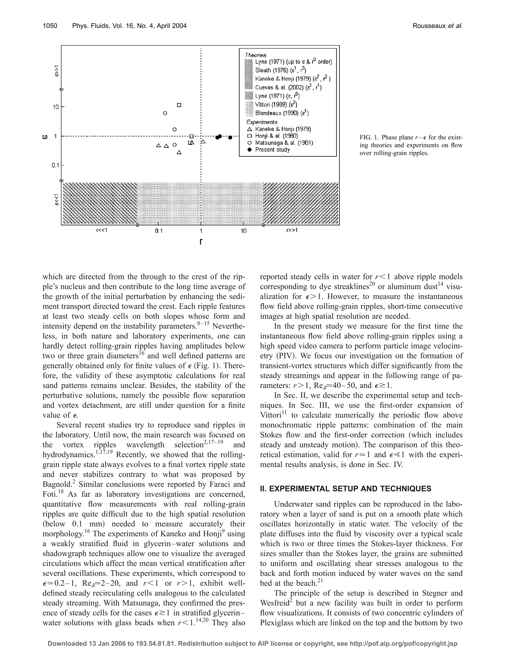
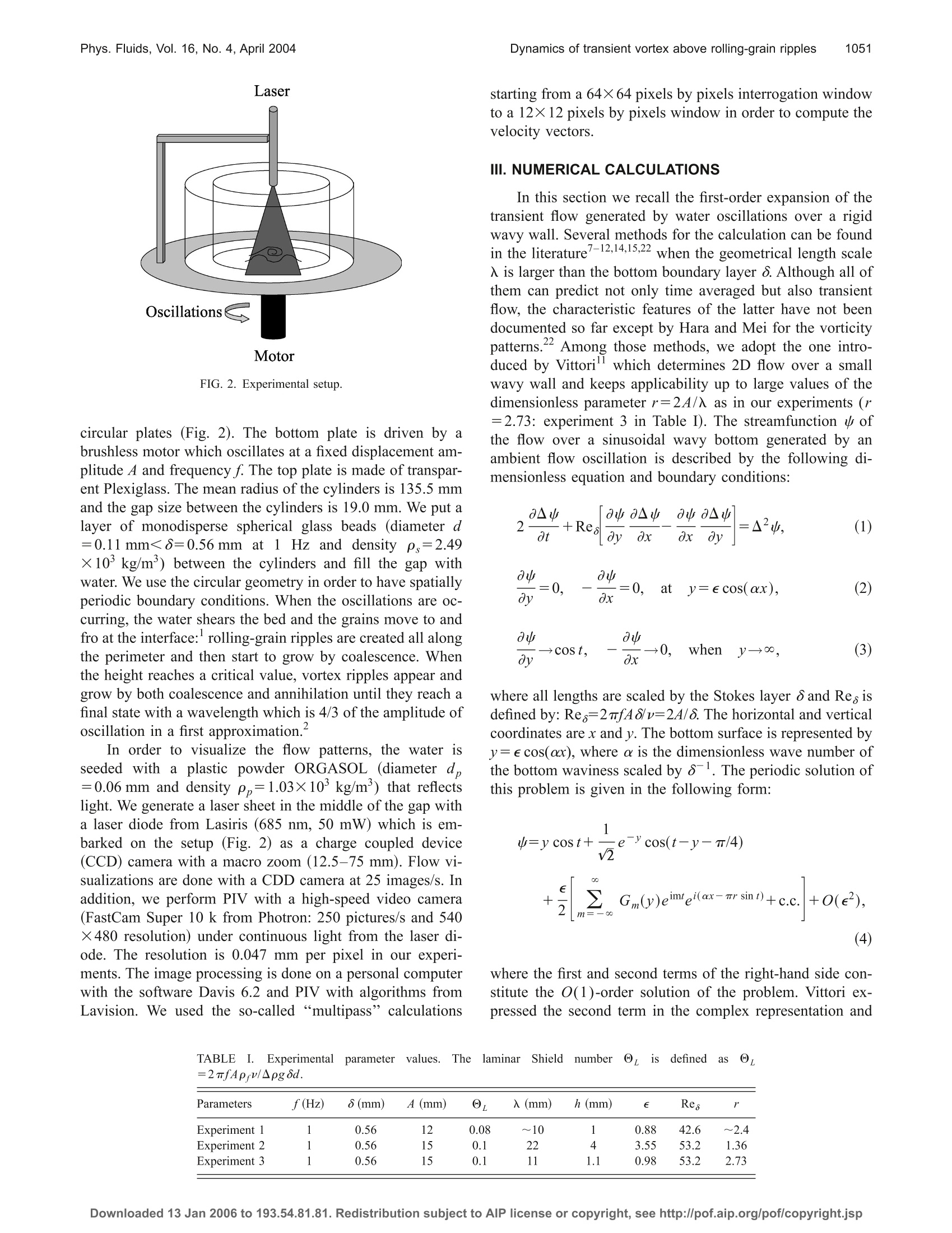
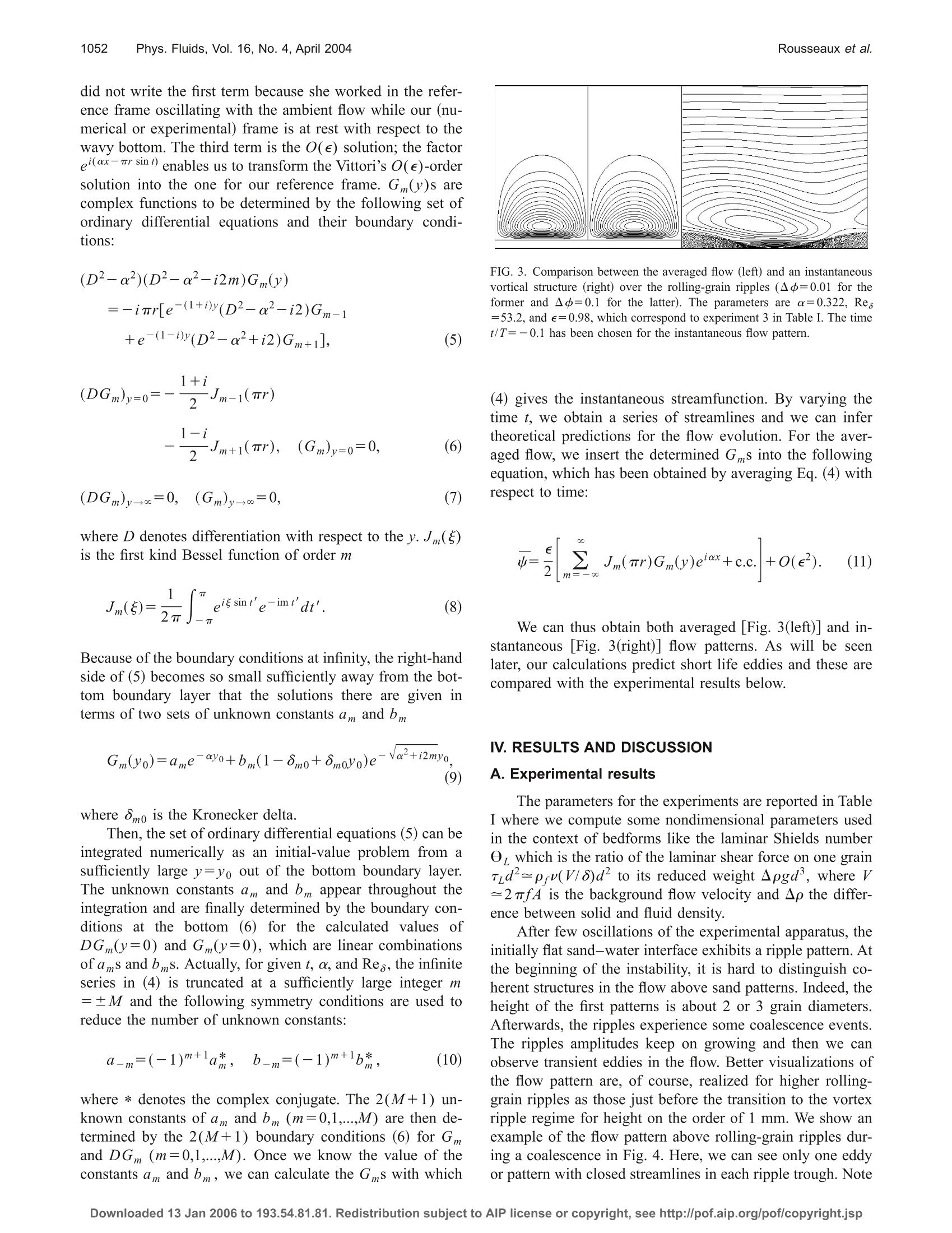
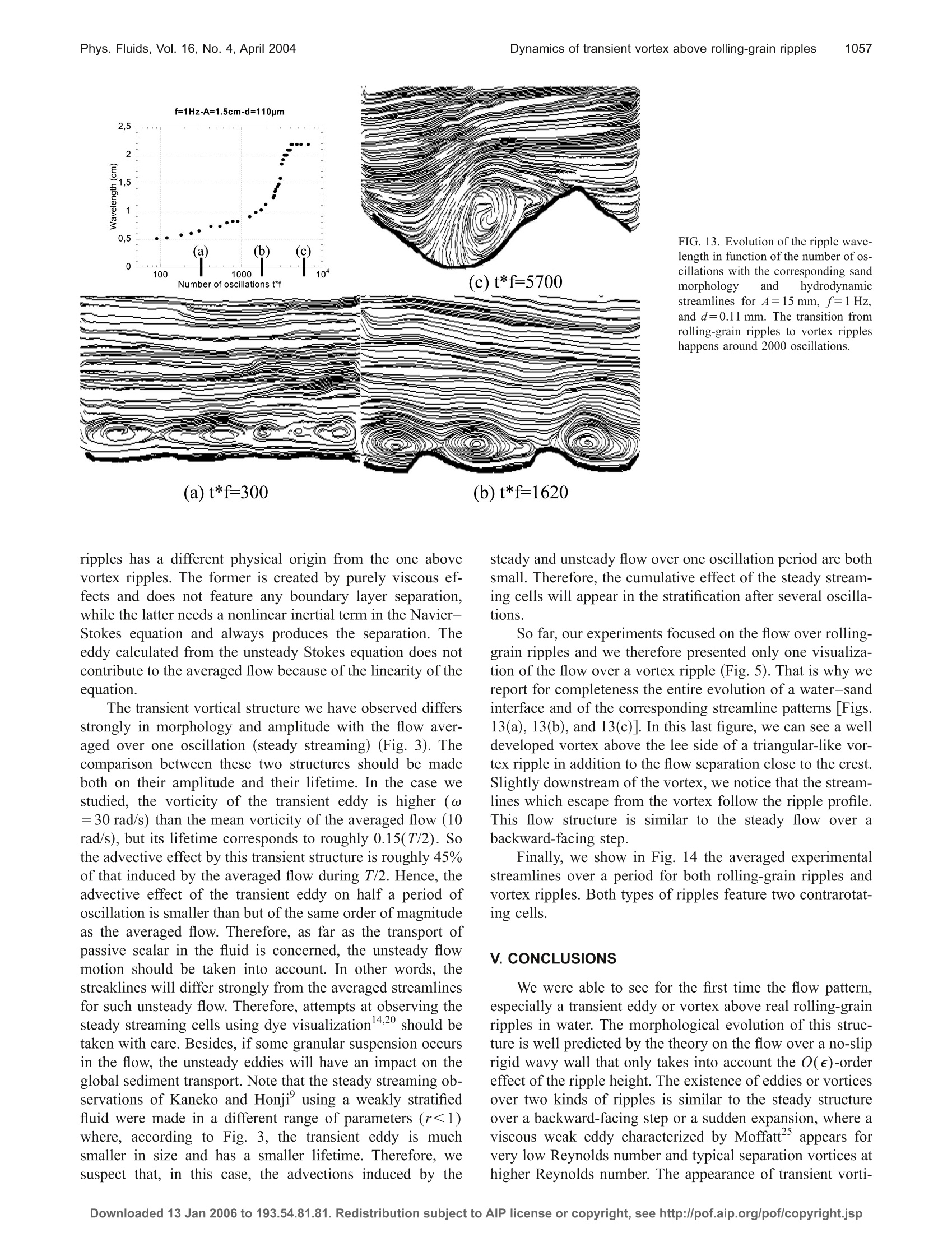
HTML RBSTRRCT+ LInKSVOLUME 16， NUMBER 4APRIL 2004 1050Phys.Fluids， Vol. 16， No. 4， April 2004Rousseaux et al. PHYSICS OF FLUIDS Dynamics of transient eddy above rolling-grain ripples Germain Rousseaux and Harunori Yoshikawab) Physique et Mecanique des Milieux Heterogenes， UMR 7636 CNRS-ESPCI， 10 Rue Vauquelin，75231 Paris Cedex 05， France Alexandre Stegner Laboratoire de Meteorologie Dynamique， ENS， 24 Rue Lhomond， 75005 Paris， France Jose Eduardo Wesfreidd) Physique et Mecanique des Milieux Heterogenes， UMR 7636 CNRS-ESPCI， 10 Rue Vauquelin，75231 Paris Cedex 05， France (Received 30 June 2003； accepted 8 January 2004；published online 8 March 2004) This study deals with the flow motion over the so-called rolling-grain ripples which are generatedby water oscillations above a sand bed. We focus our efforts on quantifying by means of laboratoryexperiments and numerical calculations the morphology and the dynamics of transient flow patterns.We report， for the first time， on the formation of an unsteady pattern with closed streamlines (we callit “eddy”) above rolling-grain ripples using flow visualizations and particle image velocimetrymeasurements. This structure appears in the ripple trough during flow reversal and scales with theripple wavelength. The experimental results are in qualitative agreement with the perturbative flowsolution calculated by Vittori in 1989. Even if the relative ripple amplitude is not small in theexperiment the perturbative expansion at the first order gives an accurate description of the flowdynamics. 2004 American Institute of Physics.[DOI： 10.1063/1.1651482] I. INTRODUCTION Ripples are very fascinating patterns which occur onsandy beaches and are created by the back and forth motioninduced by gravity waves in the water. Since the seminalwork of Bagnold， two types of patterns have been distin-guished： rolling-grain ripples and vortex ripples. Bagnold in-troduced this terminology to describe small patterns withgrains moving to and fro at the interface between sand andwater (the rolling-grain ripples) and larger patterns with avortex detaching from the crest scooping grains from theneighboring sand structures (the vortex ripples). Since then，the appearance of transient vortices above a ripple bed isgenerally assumed to be the dynamical signature of the vor-tex ripple pattern. This typical pattern corresponds to a largeamplitude perturbation of the initially flat sand bed with amaximum slope close to the avalanche angle of the granularmedium. The large angle of the pattern is assumed to beresponsible for the flow separation behind the crest whichinduces the vortex formation.On the other hand， rolling-grain ripples correspond to weak perturbations of the sandybottom having small slopes. In this limit， asymptotic expan-sion could be used to estimate theoretically the first-ordercorrection to the flow field induced by an infinitely smallwavy wall below an oscillating Stokes layer. In the two dimensional (2D) infinite-depth case，one can ( Present a d dress： I n stitut N on-Li n eaire de N i ce， S o phia-Antipolis， U M R 6618 CN R S， 1361 rou t e des Luc i oles， 06560 Valbonne， France； electronic m ail： germain.rousseaux@inln.cnrs.fr Electronic m ail： harunori@pmmh.espci.fr "Electronic m ail： s tegner@lmd.ens.fr "Electronic mail： wesfreid@pmmh.espci.fr ) describe the problem with only three dimensionless param-eters： E， Res， and r where e is half the ripple height h scaledby the Stokes layer thickness 8=√u/mf， Re， the Reynoldsnumber defined with 8， and r the ratio of the fluid displace-ment 2A to the bottom wavelength 入： e=h/28， Re；=2A/8，and r=2A/， where v is the kinematic viscosity and f theoscillation frequency. We illustrate in Fig. 1 the range of theparameters e and r corresponding to both previous andpresent works. The coupling between the frequency of the main Stokesflow and the intrinsic frequency induced by the wavy bottomperturbation generates a steady-flow component. Such a phe-nomenon is often encountered in oscillatory flow and isknown as steady streaming.4-6Lyne’ investigated the prob-lem for the case of small height e<1 and r>1 or r<1 andhe showed that a solid wavy wall could create steady recir-culations directed from the troughs to the crests. Sleathpointed out that rolling-grain ripples can be produced bysuch steady secondary flows. Kaneko and Honji’consideredhigher-order solutions in the parameter e under the conditionthat the fluid displacement is very small (r<1). Recently，Cuevas et al. obtained analytical results using a double ex-pansion in the parameter r ande (r<1 and e<1). Theyperformed this study when a vertical magnetic field acting onan electrical conducting liquid damps the steady streamings.However， as noticed by Sleath， natural ripples form for val-ues of r of order one. Therefore， Blondeaux and Vittori1-13extended the theoretical analysis for arbitrary value of rwhen e<1. Performing a standard linear stability analysis，Blondeaux explained the formation of rolling-grain ripplesby the following mechanism：2 small perturbations of theinitial flat bed creates recirculating cells (steady streamings) FIG. 1. Phase plane r-e for the exist-ing theories and experiments on flowover rolling-grain ripples. which are directed from the through to the crest of the rip-ple’s nucleus and then contribute to the long time average ofthe growth of the initial perturbation by enhancing the sedi-ment transport directed toward the crest. Each ripple featuresat least two steady cells on both slopes whose form andintensity depend on the instability parameters.8-15 Neverthe-less， in both nature and laboratory experiments， one canhardly detect rolling-grain ripples having amplitudes belowtwo or three grain diameters and well defined patterns aregenerally obtained only for finite values of e (Fig. 1). There-fore， the validity of these asymptotic calculations for realsand patterns remains unclear. Besides， the stability of theperturbative solutions， namely the possible flow separationand vortex detachment， are still under question for a finitevalue of e. Several recent studies try to reproduce sand ripples inthe laboratory. Until now， the main research was focused onthe vortex rippleswavelength selection2，17-19 andhydrodynamics.1，17，19 Recently， we showed that the rolling-grain ripple state always evolves to a final vortex ripple stateand never stabilizes contrary to what was proposed byBagnold. Similar conclusions were reported by Faraci andFoti.8 As far as laboratory investigations are concerned，quantitative flowmeasurementswithl realalIrolling-grainripples are quite difficult due to the high spatial resolution(below 0.11mm)a)needed tomeasure accuratelyr theirmorphology.16 The 9experiments of Kaneko and Honji’usinga weakly stratified fluid in glycerin-water solutions andshadowgraph techniques allow one to visualize the averagedcirculations which affect the mean vertical stratification afterseveral oscillations. These experiments， which correspond toe=0.2-1， Re；-2-20， and r<1 or r>1， exhibit well-defined steady recirculating cells analogous to the calculatedsteady streaming.With Matsunaga， they confirmed the pres-ence of steady cells for the cases e1 in stratified glycerin-water solutions with glass beads when r<1.14，20 They also reported steady cells in water for r<1 above ripple modelscorresponding to dye streaklines2 or aluminum dust4 visu-alization for e>1. However， to measure the instantaneousflow field above rolling-grain ripples， short-time consecutiveimages at high spatial resolution are needed. In the present study we measure for the first time theinstantaneous flow field above rolling-grain ripples using ahigh speed video camera to perform particle image velocim-etry (PIV). We focus our investigation on the formation oftransient-vortex structures which differ significantly from thesteady streamings and appear in the following range of pa-rameters： r>1， Re；-40-50， and e之1. In Sec. II， we describe the experimental setup and tech-niques. In Sec. II， we use the first-order expansion ofVittori to calculate numerically the periodic flow abovemonochromatic ripple patterns： combination of the mainStokes flow and the first-order correction (which includessteady and unsteady motion). The comparison of this theo-retical estimation， valid for r=1 and e<1 with the experi-mental results analysis， is done in Sec. IV. II. EXPERIMENTAL SETUP AND TECHNIQUES Underwater sand ripples can be reproduced in the labo-ratory when a layer of sand is put on a smooth plate whichoscillates horizontally in static water. The velocity of theplate diffuses into the fluid by viscosity over a typical scalewhich is two or three times the Stokes-layer thickness. Forsizes smaller than the Stokes layer， the grains are submittedto uniform and oscillating shear stresses analogous to theback and forth motion induced by water waves on the sandbed at the beach.21 The principle of the setup is described in Stegner andWesfreid but a new facility was built in order to performflow visualizations. It consists of two concentric cylinders ofPlexiglass which are linked on the top and the bottom by two Laser circular plates (Fig. 2). The bottom plate is driven by abrushless motor which oscillates at a fixed displacement am-plitude A and frequency f. The top plate is made of transpar-ent Plexiglass. The mean radius of the cylinders is 135.5 mmand the gap size between the cylinders is 19.0 mm. We put alayer of monodisperse spherical glass beads (diameter d=0.11 mm<8=0.56mm at 1 Hz and density ps=2.49×10kg/m’) between the cylinders and fill the gap withwater. We use the circular geometry in order to have spatiallyperiodic boundary conditions. When the oscillations are oc-curring， the water shears the bed and the grains move to andfro at the interface： rolling-grain ripples are created all alongthe perimeter and then start to grow by coalescence. Whenthe height reaches a critical value， vortex ripples appear andgrow by both coalescence and annihilation until they reach afinal state with a wavelength which is 4/3 of the amplitude ofoscillation in a first approximation. In order to visualize the flow patterns， the water isseeded with a plastic powder ORGASOL (diameter d，=0.06 mm and density pp=1.03×10kg/m’) that reflectslight. We generate a laser sheet in the middle of the gap witha laser diode from Lasiris (685 nm， 50 mW) which is em-barked on the setup (Fig. 2) as a charge coupled device(CCD) camera with a macro zoom (12.5-75 mm). Flow vi-sualizations are done with a CDD camera at 25 images/s. Inaddition， we perform PIV with a high-speed video camera(FastCam Super 10 k from Photron： 250 pictures/s and 540×480 resolution) under continuous light from the laser di-ode. The resolution is 0.047 mm per pixel in our experi-ments. The image processing is done on a personal computerwith the software Davis 6.2 and PIV with algorithms fromLavision. We used the so-called “multipass” calculations starting from a 64×64 pixels by pixels interrogation windowto a 12×12 pixels by pixels window in order to compute thevelocity vectors. III.NUMERICAL CALCULATIONS In this section we recall the first-order expansion of thetransient flow generated by water oscillations over a rigidwavy wall. Several methods for the calculation can be foundin the literature7-12，14，15，22 when the geometrical length scale入 is larger than the bottom boundary layer 8. Although all ofthem can predict not only time averaged but also transientflow， the characteristic features of the latter have not beendocumented so far except by Hara and Mei for the vorticitypatterns."? Among those methods， we adopt the one intro-duced by Vittori which determines 2D flow over a smallwavy wall and keeps applicability up to large values of thedimensionless parameter r=2A/入 as in our experiments (r=2.73： experiment 3 in Table I). The streamfunction w ofthe flow over a sinusoidal wavy bottom generated by anambient flow oscillation is described by the following di-mensionless equation and boundary conditions： where all lengths are scaled by the Stokes layer and Reg isdefined by： Re=2mfA8/v=2A/8. The horizontal and verticalcoordinates are x and y. The bottom surface is represented byy=e cos(ox)， where a is the dimensionless wave number ofthe bottom waviness scaled by 8-1. The periodic solution ofthis problem is given in the following form： where the first and second terms of the right-hand side con-stitute the O(1)-order solution of the problem. Vittori ex-pressed the second term in the complex representation and TABLEI.1.EExperimentalparameterrvalues.. .TThelaminar Shield number @Lis defined as O，=2mfApv/Apg8d. Parameters f(Hz) 8(mm) A (mm) 入 (mm) h (mm) E Re； Experiment 1 1 0.56 12 0.08 ~10 1 0.88 42.6 ~2.4 Experiment 2 0.56 15 0.1 22 4 3.55 53.2 1.36 Experiment 3 1 0.56 15 0.1 11 1.1 0.98 53.2 2.73 did not write the first term because she worked in the refer-ence frame oscillating with the ambient flow while our (nu-merical or experimental) frame is at rest with respect to thewavy bottom. The third term is the O(e) solution； the factorei(ax-mr sin t) enables us to transform the Vittori’s O(e)-ordersolution into the one for our reference frame. Gm()s arecomplex functions to be determined by the following set ofordinary differential equations and their boundary condi-tions： where D denotes differentiation with respect to the y. Jm(5)is the first kind Bessel function of order m Because of the boundary conditions at infinity， the right-handside of (5) becomes so small sufficiently away from the bot-tom boundary layer that the solutions there are given interms of two sets of unknown constants am and bm (9) where 8mo is the Kronecker delta. Then， the set of ordinary differential equations (5) can beintegrated numerically as an initial-value problem from asufficiently large y=yo out of the bottom boundary layer.The unknown con)wnstants am and bm appear throughout theintegration and are finally determined by the boundary con-ditions at the bottom (6) for the calculated values ofDGm(y=0) and Gm(y=0)， which are linear combinationsof ams and bms. Actually， for given t， a， and Res，the infiniteseries in (4) is truncated at a sufficiently large integer m=±M and the following symmetry conditions are used toreduce the number of unknown constants： where * denotes the complex conjugate. The 2(M+1) un-known constants of am and bm(m=0，1，...，M) are then de-termined by the 2(M+1) boundary conditions (6) for Gmand DGm (m=0，1，...，M). Once we know the value of theconstants am and bm， we can calculate the Gms with which FIG. 3. Comparison between the averaged flow (left) and an instantaneousvortical structure (right) over the rolling-grain ripples (Ab=0.01 for theformer and ▲d=0.1 for the latter). The parameters are α=0.322， Re，=53.2， and e=0.98， which correspond to experiment 3 in Table I. The timet/T=-0.1 has been chosen for the instantaneous flow pattern. (4) gives the instantaneous streamfunction. By varying thetime t， we obtain a series of streamlines and we can infertheoretical predictions for the flow evolution. For the aver-aged flow， we insert the determined Gms into the followingequation， which has been obtained by averaging Eq. (4) withrespect to time： We can thus obtain both averaged [Fig. 3(left)] and in-stantaneous [Fig. 3(right)]flow patterns. As will be seenlater， our calculations predict short life eddies and these arecompared with the experimental results below. IV. RESULTS AND DISCUSSION A. Experimental results The parameters for the experiments are reported in TableI where we compute some nondimensional parameters usedin the context of bedforms like the laminar Shields numberO， which is the ratio of the laminar shear force on one graind'=p(V/8)d"to its reduced weight Apgd， where V=2mfA is the background flow velocity and Ap the differ-ence between solid and fluid density. After few oscillations of the experimental apparatus， theinitially flat sand-water interface exhibits a ripple pattern. Atthe beginning of the instability， it is hard to distinguish co-herent structures in the flow above sand patterns. Indeed， theheight of the first patterns is about 2 or 3 grain diameters.Afterwards， the ripples experience some coalescence events.The ripples amplitudes keep on growing and then we canobserve transient eddies in the flow. Better visualizations ofthe flow pattern are， of course， realized for higher rolling-grain ripples as those just before the transition to the vortexripple regime for height on the order of 1 mm. We show anexample of the flow pattern above rolling-grain ripples dur-ing a coalescence in Fig. 4. Here， we can see only one eddyor pattern with closed streamlines in each ripple trough. Note FIG.4. Visualization of the flow pat-tern over rolling-grain ripples during acoalescence for A=12 mm， f=1 Hz，and d=0.11 mm. that the horizontal extension of the eddies over rolling-grainripples is fixed by the distance between two ripple crests.The experimental flow parameters here are e=0.88， Re=42.5， and r=2.4 corresponding to experiment 1 (see TableI). Later in time rolling-grain ripples experience a transitionto the vortex ripple regime. During this transition， the ripplesgrow rapidly， accompanyingttheeappearance of largevortices. The ripples finally reach a relatively fixed statewhich slightly evolves on very long times. We can observe avortex detaching from each ripple crest twice during oneoscillation period. Unlike the transient eddies described inFig. 4， the horizontal vortex size over vortex ripples isroughly equal to half a ripple wavelength (Fig. 5 for e=3.55， Re；=53.2， andr=1.36， corresponding to experiment2 of Table I). An important characteristic of the eddies observed aboverolling-grain ripples is that they are short lived. These tran-sient structures appear while the flow reverses its direction ofmotion. Unlike the vortex-ripples vortices as the one shownin Fig. 5， these eddies remain coherent for only a very shorttime compared to half of the ambient-flow oscillation periodT/2. From the PIV， we compute the velocity vectors of thesetransient structures over rolling-grain ripples (Fig. 6) and wecan display the associated streamlines. Indeed， instantaneous streamlines showing the dynami-cal evolution of these eddies are presented in Fig. 7. Heree=0.98， Re；=53.2， and r=2.73 corresponding to experi-ment 3 in Table I (note the difference of scalings betweenexperimental and theoretical images in Figs. 7 and 8 as men-tioned in the legends). In this case， the observed eddy re-mains coherent for roughly 70 ms， that is to say， around oneseventh of T/2 (T=1s). In contrast with the steady cellsshown in Kaneko and Honji by glycerin-water stratifica-tion， the observed transient cells exist one per trough， coro-tating together. Each of them occupies all length over atrough and has a vertical size around twice the ripple height[Fig. 7(b)]. It grows vertically and then is ejected from thebottom. After the ejection， the elliptical eddy deforms itsshape as shown in Fig. 8(a). We note here that the verticalposition of the eddy’s center seems to follow the flow rever-sal line of the unperturbed Stokes layer. After the ambientflow reversal， this structure disappears in a very short time.Then， a simple unidirectional shearing can be seen. The ob-servation of the eddy’s birth is difficult due to its size， whichis on the order of the Stokes layer. Besides，the settled plasticparticles and disturbed sand grains introduce a large scalenoise on the video image which affects the PIV resolution.Sometimes we notice that the eddy appears on the lee side of FIG. 5. Visualization of the flow pat-tern over a vortex ripple for A=15 mm， f=1Hz， d=0.11 mm： wesuperimposed four successive imagestaken at 250 pictures/ps. The back-ground flow goes to the left. FIG. 6. Velocity vectors of the tran-sient eddies aboverolling grainsripples for A=15 mm， f=1Hz， d=0.11 mm， t*f=1620 (number of os-cillations)， and 32 ms before flow re-versal. The background flow goes tothe right. ripples and grows horizontally to occupy the whole spacebetween two neighboring ripple crests. Quantitative measurements of the velocity and the vor-ticity of the transient eddy corresponding to Fig. 7(b) areobtained from the PIV. For this case， the maximum velocity(V=23 mm/s) and vorticity (ω=28 rad/s) of the eddy re-mains smaller than the maximum velocity (V=95 mm/s)and vorticity (ω=167 rad/s) of the main oscillating Stokesflow. Hence， even if the relative ripple height e=0.98 isclose to unity， the amplitude of the perturbed flow (i.e.， ve- =15 mm， f=1Hz， d=0.11 mm， and t*f=1620 (number of oscillations).Experimental and numerical streamlines with the Stokes background flowprofile (At=16 ms). (a) is 60 ms before flow reversal. For the experimental(numerical) images， the height is 4.1 mm and the width is 24.5 mm (11mm). The background flow goes to the right. locity and vorticity of the transient vortex) would be lessthan one third of the maximum unperturbed Stokes flow. B. Numerical results and comparisons Numerical calculations with different parameter valuesin the regime r>1 predict the appearance of one eddy orstructure with closed streamlines above each ripple troughtwice during an ambient flow oscillation. We show， on theright half of Figs. 7 and 8， the calculated streamlines havingthe same parameters (e=0.98， Re；=53.2， and r=2.73) as FIG. 8. Ejection and death of the eddy over the rolling-grain ripples for A=15 mm， f=1Hz， d=0.11 mm， and t*f=1620 (number of oscillations).Experimental and numerical streamlines with the Stokes background flowprofile (At=8 ms). (d) is 4 ms before flow reversal. For the experimental(numerical) images， the height is 4.1 mm (7.7 mm) and the width is 24.5mm (11 mm). FIG. 9. Position of the eddy’s center for A=15 mm， f=1Hz， d=0.11 mm， and t*f=1620 (number of oscillations). t=0 corresponds toflow reversal. the experiment. We have truncated the series (4) at M=25 tocalculate the numerical streamlines and compared them withthe experimental ones at the same instant. The velocity pro-files of the unperturbed Stokes flow above a flat bottom arealso shown in the middle of Figs. 7 and 8. Surprisingly， even if the validity of the asymptotic ex-pansion (detailed in Sec. III) is seemingly in question for e=1， the first-order calculation seems to capture correctly thedynamics of the transient eddy observed in the experiment.In Fig. 7(a)， we can see an eddy turning clockwise above thetrough. It occupies the whole length over the ripple troughand its center is located above the midthrough slightly up-stream. The calculated transient vorticity (ω=30 rads) isin very good agreement with the vorticity estimated in theexperiment (ω=28 rads). This eddy stays in the middleof the trough while it grows along the vertical. Then， it isdeformed towards the upstream left crest [Figs. 7(b) and7(c)]. After this growth process， the eddy is ejected and sig-nificantly deformed， enlarging vertically again. The centershifts upstream as it rises [Fig. 8(a)]. This ejected eddy sig-nificantly deforms to a quasitriangular shape just after theambient flow reversal [Fig.8(b)]. Then， the eddy disappearswithin a very short time. It rapidly shrinks and disappears[Fig. 8(c)] within a layer of thickness approximately equal to入/3. In order to quantify more precisely the dynamics of thistransient structure， we have plotted its vertical and horizontalpositions (Fig. 9) as well as its path over the ripple through(Fig. 10). The zero for the horizontal (vertical) position cor-responds to the left crest (the mid height of the ripple). As faras the eddy’s position is concerned， there is a correct agree-ment between the numerical calculation and the laboratoryobservations， even if the theoretical predictions slightly over-estimate the vertical and the horizontal positions. Besides，the first-order expansion gives important results about thisposition at the very beginning of the eddy’s appearancewhich cannot be detected in the experiments. In particular，one can observe a clear increase of the horizontal position atthe beginning before reaching a plateau close to the center of FIG. 10. Trajectory of the eddy’s center for A=15 mm， f=1Hz， d=0.11 mm， and t*f=1620 (number of oscillations). the ripple trough. Afterwards， the eddy’s center is shiftedupstream before its death (Fig. 10). It is important to notethat the calculated positions do not depend on the value of e(Fig. 9). Hence， the eddy’s path will be the same for bothsmall and finite ripple amplitudes. In fact， the vertical posi-tion of the eddy follows the null-velocity position of theunperturbed Stokes flow. Nevertheless some discrepancies appear between the cal-culated and observed streamlines. The asymptotic expansionpredicts a strong reverse shear below the transient eddywhich is not observed in the experiment. Besides， thesestreamlines intersect the ripple interface， which correspondto a nonphysical transverse velocity. Hence， the validity ofthe first order expansion is broken for the boundary conditionwhen e reaches a finite value. Unlike the analytical model，the experimental shape of the ripple is not sinusoidal. Thiscould also introduce some discrepancies between the calcu-lated and observed streamlines. Moreover， we assumed a no-slip boundary condition in the calculations， whereas a smallslip velocity at the interface between a fluid and a porousmedia could occur.23，24 Unlike laboratory measurements which have limitedresolution， the numerical calculations give information onthe initial generation of the transient eddy along the bottomStokes boundary layer. The eddy generates at a very smallsize on the lee side of ripple crests and enlarges horizontallyto occupy all the wavelength over the ripple trough. Thisprocess could not be observed clearly in our experimentsbecause of the size of the Stokes layer， which is about 8=0.56mm in water at 1 Hz. For the observation on scalecomparable to the wavelength 入，the appearance over thetrough is very well predicted. Figure 11 shows this processfor the parameters of experiment 3 in Table I except for thevalue of e which is 0.1. The calculations for r<1 also show transient structuresduring the ambient flow reversal. Parameter dependence ofthe transient flow structure with r is shown in Fig. 12 at19T/250 before the ambient flow reversal for a=0.322 ande=0.1. The predicted morphology is very different. Two ed- FIG. 11. Birth of the eddy over the rolling-grain ripples for the followingparameters： a=0.322， r=2.73， and e=0.1. The time t=0 corresponds toflow reversal. The background flow goes to the right. dies are generated at the crest and trough， respectively， andboth are ejected vertically [Fig. 12(a)]. They merge into onelarger eddy above the crest and disappear over the crest.Between the former (r>1) and latter (r<1) parameter re-gimes， we have an intermediate one [Fig. 12(b)]， where we 0 0 FIG. 12. Dependence of the flow morphology on the r parameter with a=0.322 and e=0.1 at 19T/250 before the ambient flow reversal from theright to the left. The background flow goes to the right. observe the fusion of two eddies above the ripple lee side.Whether one or two eddies appear would depend on r (noticethat we always keep the condition 入> 8). In our numericalexplorations of the total flow， we always see one vorticalstructure when r>1 and when r is smaller than 1， we ob-served the merging of two eddies into a larger one. Thiscriterion enables us to distinguish the two regimes and hassome relation with Vittori's criterion on the number of steadyrecirculating cells. Indeed， the curve r=1 is similar to thelimiting curve of the (a， Res) plane in Fig. 8 of Ref. 11 forthe case of Re；>10， which corresponds to real ripples inwater (we recall that aRs=2Tr). C. Discussion Several questions arise from this combined theoreticaland experimental investigation. First of all， how far can werely on the asymptotic calculations of the perturbed flow?Why do these calculations capture correctly the transient vor-tex dynamic in the range of e=1 where the validity of theexpansion is in principle broken? In fact， one should keep in mind that the dimensionlesswave number a is also a small parameter and that the per-turbed flow is controlled both by the ripple height e and theripple wavelength a. Indeed， if a tends to zero (ripple wave-length tends to infinity) the perturbed flow should vanish，even if we keep e=1. Hence， we can suspect that the ampli-tude of the transient eddy scales with the ripple slope aerather than relative ripple height e. First-order expansionscould be extended up to a large value of e if the ripple sloperemains small enough. Moreover， we should note that thecorrect agreement between the laboratory observation andthe theoretical solution shows that this asymptotic solution isrobust in the range of parameters studied with respect to theflow structure prediction despite some errors near the bottomboundary layer. Therefore， our results tend to validate the useof laminar asymptotic theory to estimate the perturbed flowabove rolling-grain ripples. To have an idea of the physical origin of this structure，thesolutions of the： unsteady Stokes equation (Ay=vA’w) have also been examined. By the same method asdescribed in Sec. II， an explicit expression for the stream-function is obtained and this streamfunction gives very simi-lar streamlines to those calculated by resolving the fullNavier-Stokes equation. By the solution of the unsteadyStokes equation， the appearance of an eddy at flow reversalis predicted and the size and form of the eddy are well de-scribed by this solution with a small difference with respectto the horizontal position of the eddy’s center. Hence， theeddies observed experimentally are caused by the viscosityand one can infer that fluid inertia does not play the mainrole during flow reversal that is at the weakest moment of theflow. It is interesting to note that these two kinds of flows areanalogous to those observed in the steady flow behind abackwards-facing step or a sudden expansion， where a purelyviscous eddy as studied by Moffatt or a vortex formed withthe flow separation at the corner of the step is observed，depending on the value of the parameters.25，26 The observed vortical structure above rolling-grain (a)t*f=300 (b) t*f=1620 FIG. 13. Evolution of the ripple wave-length in function of the number of os-cillations with the corresponding sandmorphology and hydrodynamicstreamlines for A=15 mm， f=1Hz，and d=0.11mm. The transition fromrolling-grain ripples to vortex rippleshappens around 2000 oscillations. ripples has a different physical origin from the one abovevortex ripples. The former is created by purely viscous ef-fects and does not feature any boundary layer separation，while the latter needs a nonlinear inertial term in the Navier-Stokes equation and always produces the separation. Theeddy calculated from the unsteady Stokes equation does notcontribute to the averaged flow because of the linearity of theequation. The transient vortical structure we have observed differsstrongly in morphology and amplitude with the flow aver-aged over one oscillation (steady streaming) (Fig. 3). Thecomparison between these two structures should be madeboth on their amplitude and their lifetime. In the case westudied， the vorticity of the transient eddy is higher (w=30 rad/s) than the mean vorticity of the averaged flow (10rad/s)， but its lifetime corresponds to roughly 0.15(T/2). Sothe advective effect by this transient structure is roughly 45%of that induced by the averaged flow during T/2. Hence， theadvective effect of the transient eddy on half a period ofoscillation is smaller than but of the same order of magnitudeas the averaged flow. Therefore， as far as the transport ofpassive scalar in the fluid is concerned， the unsteady flowmotion should be taken into account. In other words， thestreaklines will differ strongly from the averaged streamlinesfor such unsteady flow. Therefore， attempts at observing thesteady streaming cells using dye visualization14，20 should betaken with care. Besides， if some granular suspension occursin the flow， the unsteady eddies will have an impact on theglobal sediment transport. Note that the steady streaming ob-servations of Kaneko and Honji’ using a weakly stratifiedfluid were made in a different range of parameters (r<1)where， according to Fig. 3， the transient eddy is muchsmaller in size and has a smaller lifetime. Therefore， wesuspect that， in this case， the advections induced by the steady and unsteady flow over one oscillation period are bothsmall. Therefore， the cumulative effect of the steady stream-ing cells will appear in the stratification after several oscilla-tions. So far， our experiments focused on the flow over rolling-grain ripples and we therefore presented only one visualiza-tion of the flow over a vortex ripple (Fig.5). That is why wereport for completeness the entire evolution of a water-sandinterface and of the corresponding streamline patterns [Figs.13(a)， 13(b)， and 13(c)]. In this last figure， we can see a welldeveloped vortex above the lee side of a triangular-like vor-tex ripple in addition to the flow separation close to the crest.Slightly downstream of the vortex， we notice that the stream-lines which escape from the vortex follow the ripple profile.This flow structure is similar to the steady flow over abackward-facing step. Finally， we show in Fig. 14 the averaged experimentalstreamlines over a period for both rolling-grain ripples andvortex ripples. Both types of ripples feature two contrarotat-ing cells. V. CONCLUSIONS We were able to see for the first time the flow pattern，especially a transient eddy or vortex above real rolling-grainripples in water. The morphological evolution of this struc-ture is well predicted by the theory on the flow over a no-sliprigid wavy wall that only takes into account the O(e)-ordereffect of the ripple height. The existence of eddies or vorticesover two kinds of ripples is similar to the steady structureover a backward-facing step or a sudden expansion， where aviscous weak eddy characterized by Moffatt appears forvery low Reynolds number and typical separation vortices athigher Reynolds number. The appearance of transient vorti- FIG. 14. Averaged streamlines over a period (250 pictures/s)： (a) rolling-grain rripples(t*f=1620)； (b) vortex ripples (t*f=5700)，forr A=15 mm， f=1 Hz， and d=0.11 mm. ces above a ripple bed was generally assumed to be the dy-namical signature of vortex ripple patterns， whereas our verycareful experiments show that rolling-grain ripples also fea-ture a transient coherent hydrodynamical structure. The ex-istence of the coherent structure that was observed both ex-perimentally and numerically raises an essential questionabout the difference in the sand transport between therolling-grain ripples and the vortex ripples as both featuresuch a coherent structure during the flow reversal. Our cal-culations show that linear analysis is robust and still predictsthe eddy’s characteristics despite some discrepancies in thebottom layer for e~1. Future works should concentrate onthe role of these two different flow configurations on theerosion mechanism in each kind of ripple (rolling-grain andvortex ripples). ACKNOWLEDGMENTS We are grateful to Denis Vallet， Olivier Brouard， andChristian Baradel for technical help. This work was sup-ported by the A.C.I. “Jeunes chercheurs”Grant No. 2314.We thank S. Davis and S. Cuevas for fruitful discussions onsteady streamings. R. A. Bagnold，“Motion of waves in shallow water. Interaction betweenwaves and sand bottoms. With an additional note by Sir G. I. Taylor，"Proc. R. Soc. London， Ser. A 187， 1 (1946). A. Stegner and J.-E. Wesfreid，“Dynamical evolution of sand ripples underwater，” Phys. Rev. E 60， 3487 (1999). 'J. F. A. Sleath， Sea Bed Mechanics (Wiley， New York， 1984). “N. Riley，“Steady streaming，" Annu. Rev. Fluid Mech. 33， 43 (2001). L. Petit and P. Gondret，“Redressement d'un ecoulement alternatif，”J.Phys. II 2， 2115 (1992). °S. Cuevas and G. Huelsz，“Oscillatory boundary-layer flows，" Recent Res.Dev. Fluid Dyn. 2，35 (1999). 'W. H. Lyne，“Unsteady viscous flow over a wavy wall，”J. Fluid Mech.50， 33 (1971). J. F. A. Sleath，“On rolling-grain ripples，"J. Hydraul. Res. 14， 69 (1976).A. Kaneko and H. Honji，“Double structures of steady streaming in theoscillatory viscous flow over a wavy wall，"J. Fluid Mech. 93， 727 (1979). 1s. Cuevas， F. Z. Sierra， and A. A. Avramenko，“Magnetic damping ofsteady streaming vortices in an oscillatory viscous flow over a wavywall，”Magnetohydrodynamics (N.Y.) 38， 345 (2002). G. Vittori，“Non-linear viscous oscillatory flow over a small amplitudewavy wall，”J. Hydraul. Res. 27， 267 (1989). P. Blondeaux，“Sand ripples under sea-waves. Part 1. Ripple formation，”J. Fluid Mech. 218，1(1990). G. Vittori and P. Blondeaux，“Sand ripples under sea-waves. Part 2. Finite-amplitude development，”J. Fluid Mech. 218， 19 (1990). “N. Matsunaga， A. Kaneko， and H. Honji， “A numerical study of steadystreamings in the oscillatory flow over a wavy wall，”J. Hydraul. Res. 19，29 (1981). T. Hara and C. C. Mei，“Oscillating flow over periodic ripples，"J. FluidMech. 211， 183(1990). G. Rousseaux， A. Stegner， and J.-E. Wesfreid， “Wavelength selection ofrolling grains ripples in the laboratory” (preprint， 2003). K. Andersen， “The dynamics of ripples beneath surface waves，" Ph.D.thesis， Niels Bohr Institute， 1999 (http：//www.nbi.dk/~kenand). C. Faraci and E. Foti， “Evolution of small scale regular patterns generatedby waves propagating over a sandy bottom，” Phys. Fluids 13， 1624(2001). M. A. Scherer， F. Melo， and M. Marder，“Sand ripples in an oscillatingsand-water cell，"Phys. Fluids 11， 58 (1999). 20H. Honji， A. Kaneko， and N. Matsunaga，l.“Flow above oscillatoryripples，” Sedimentology 27， 225 (1980). E. Guyon， L. Petit， J. P. Hulin， and C. Mitescu， Physical Hydrodynamics(Oxford University Press， Oxford， 2001). 22T. Hara， C. C. Mei， and K. T. Shum， “Oscillatory flow over periodicripples of finite slope，"Phys. Fluids A 4， 1373 (1992). 2P. L. F. Liu， M. H. Davis， and S. Downing， “Wave-induced boundary layerflows above and in a permeable bed，"J. Fluid Mech. 325， 195 (1996). 24S.-C. Hsiao and P. L. F. Liu， “The porous effect on the bottom instabilityunder partially standing waves，”Chin. J. Mech. Ser. A 18， 53 (2002). 25H. K. Moffatt， “Viscous and resistive eddies near a sharp corner，"J. FluidMech. 18， 1 (1964). 26N. Alleborn， K. Nandakumar， H. Raszillier， and F. Durst， “Further contri-butions on the two-dimensional flow in a sudden expansion，”J. FluidMech. 330， 169 (1997). American Institute of Physics/$ownloaded Jan to Redistribution subject to AIP license or copyright， see http：//pof.aip.org/pof/copyright.jsp Downloaded Jan to Redistribution subject to AIP license or copyright， see http：//pof.aip.org/pof/copyright.jsp