流体,多相流,两相流,气泡流中速度矢量场检测方案(粒子图像测速)

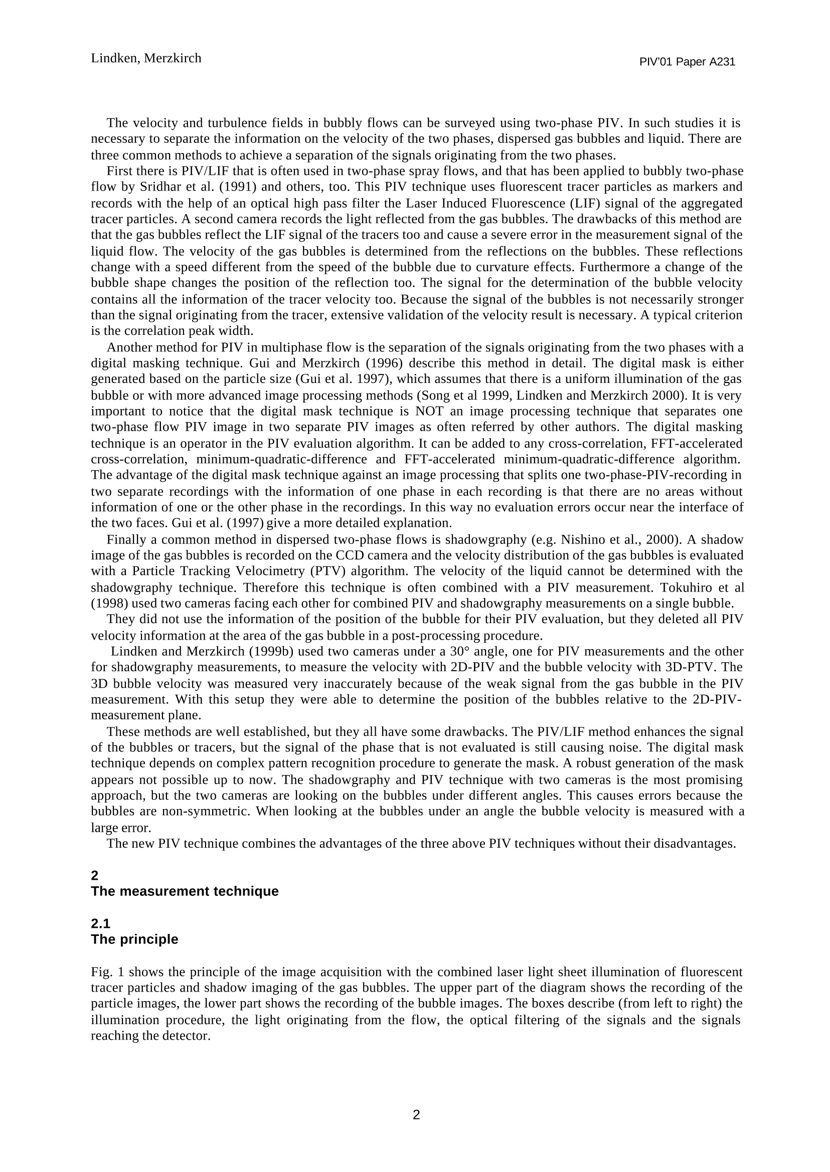
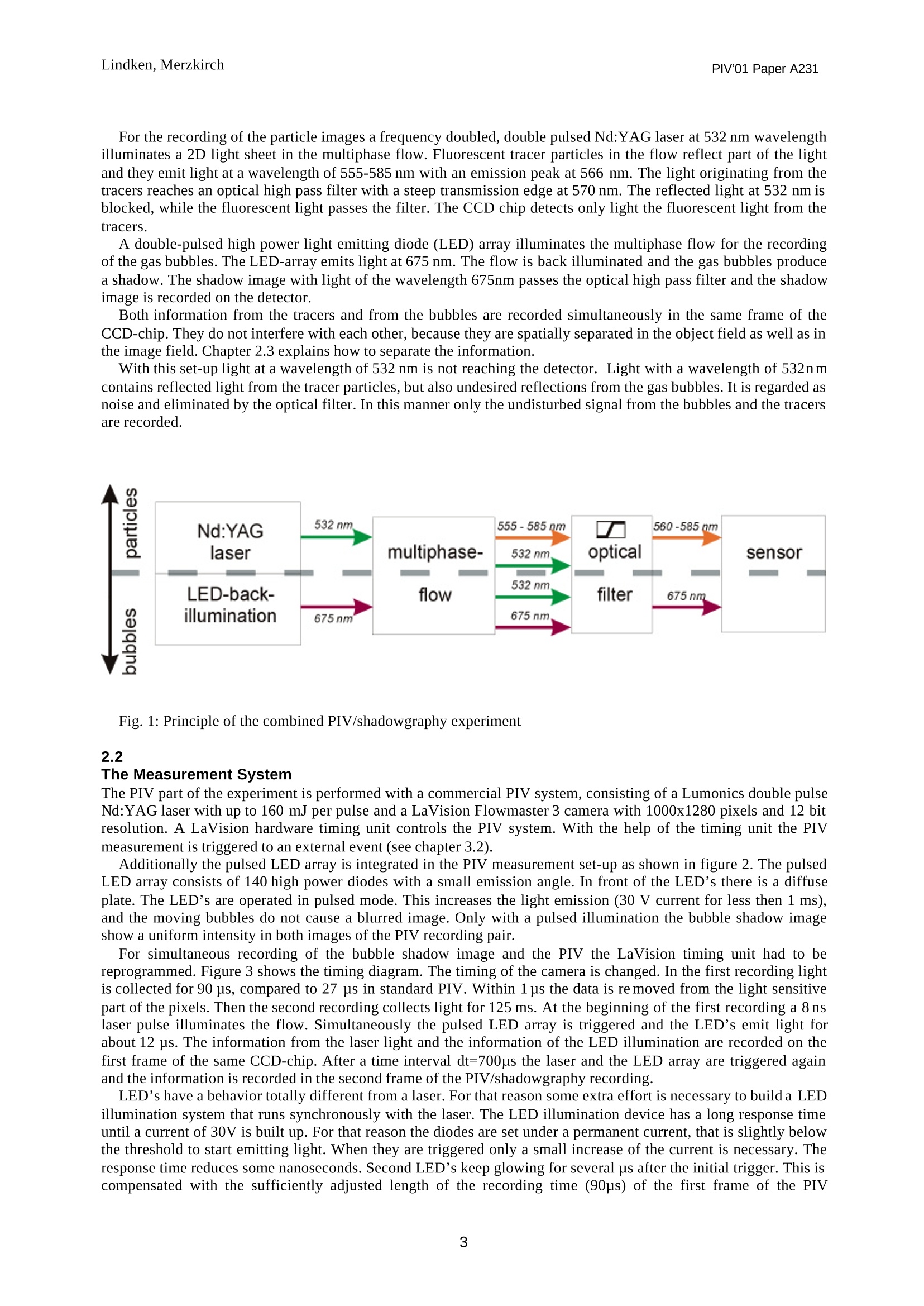
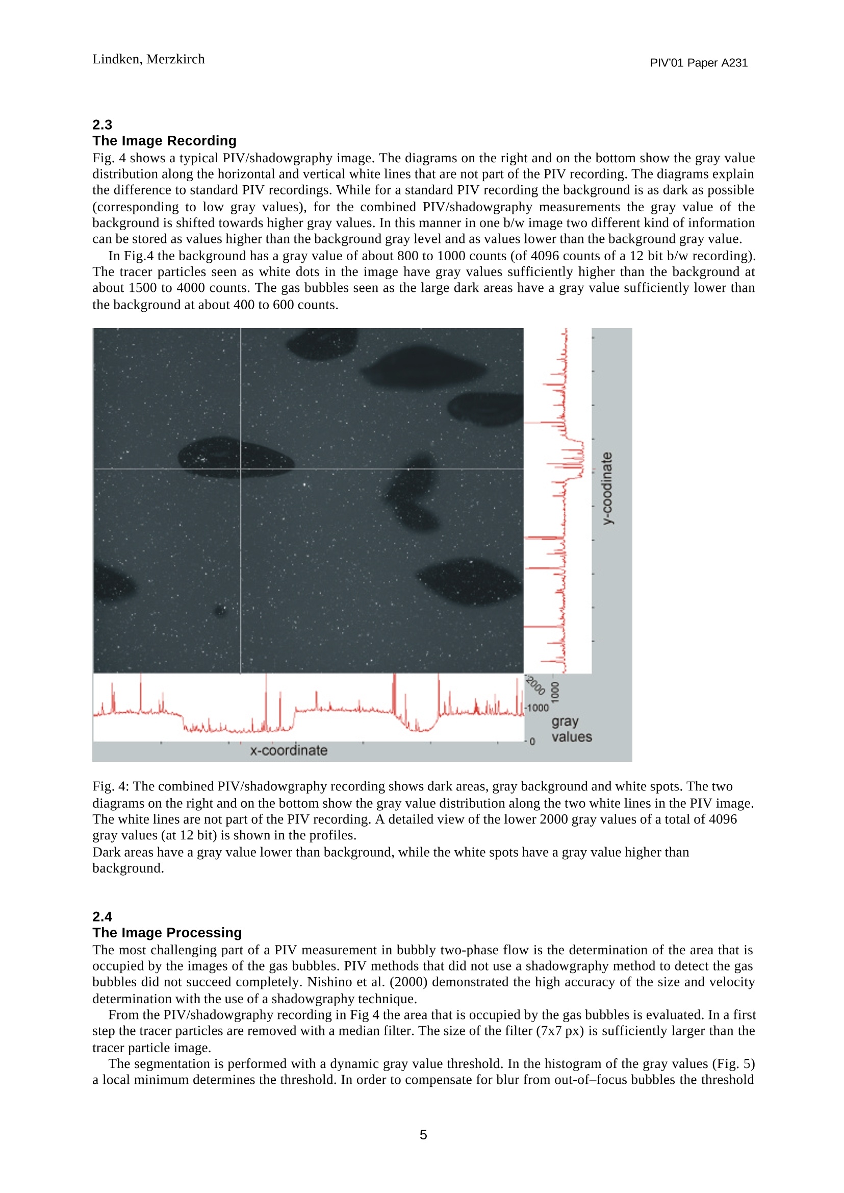
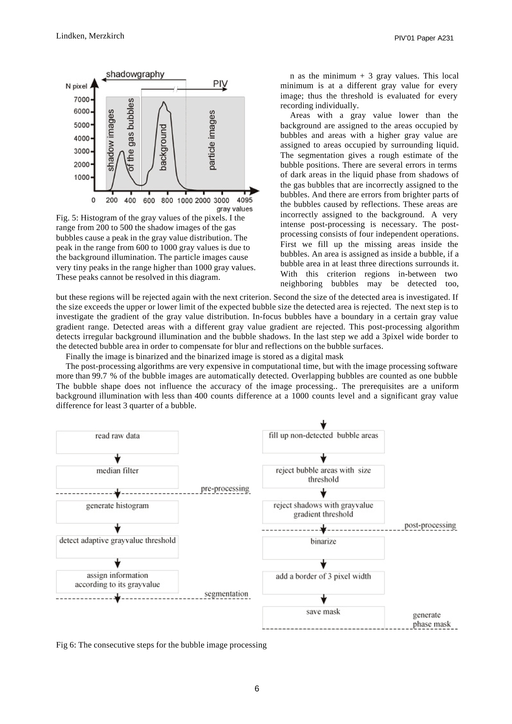
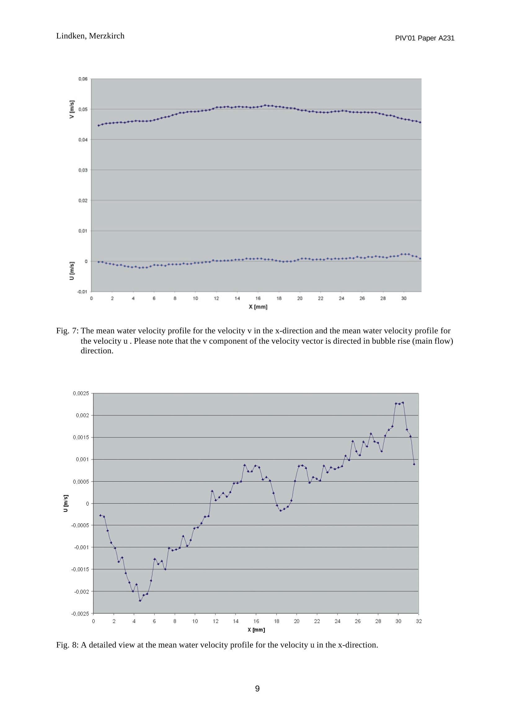
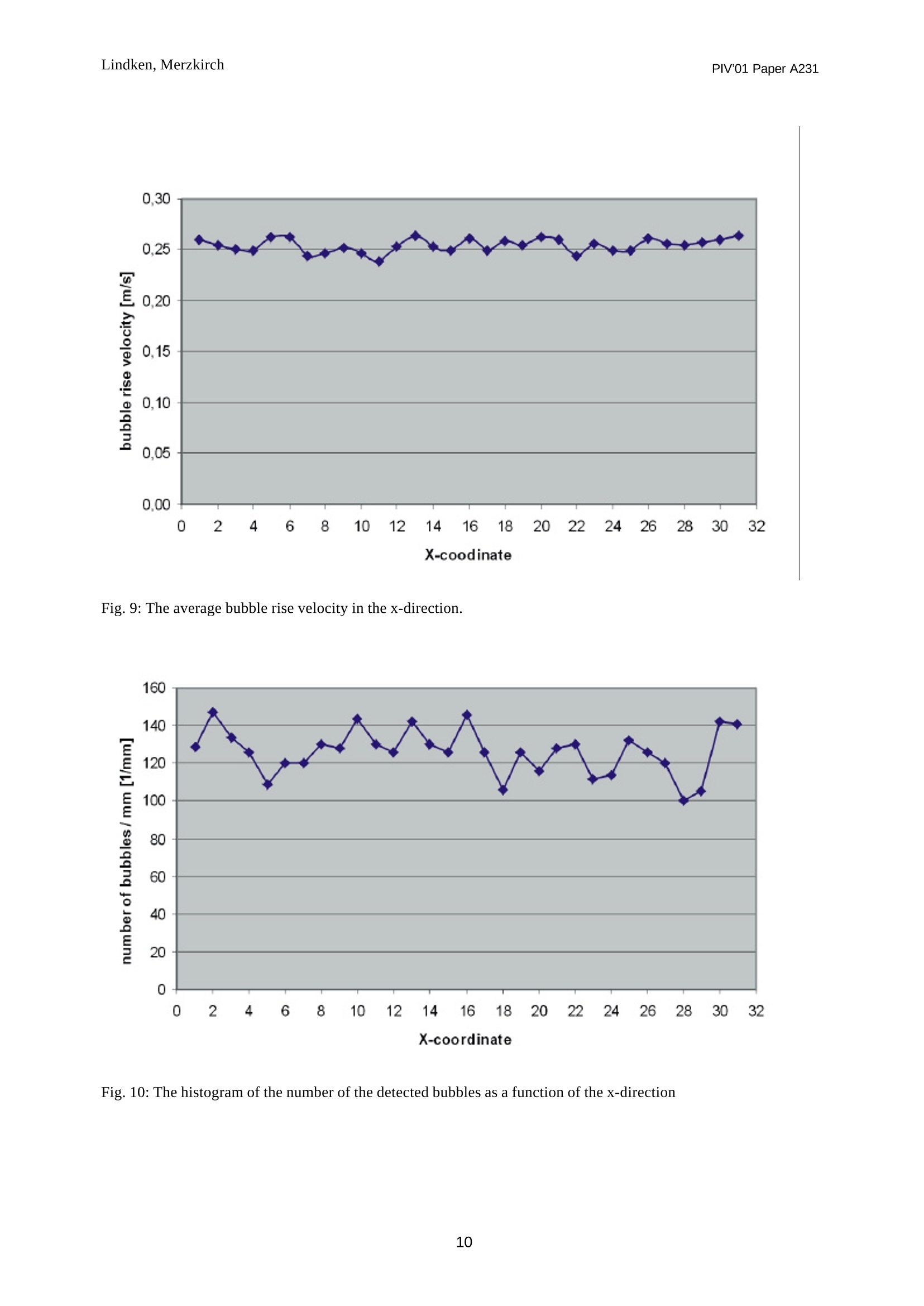
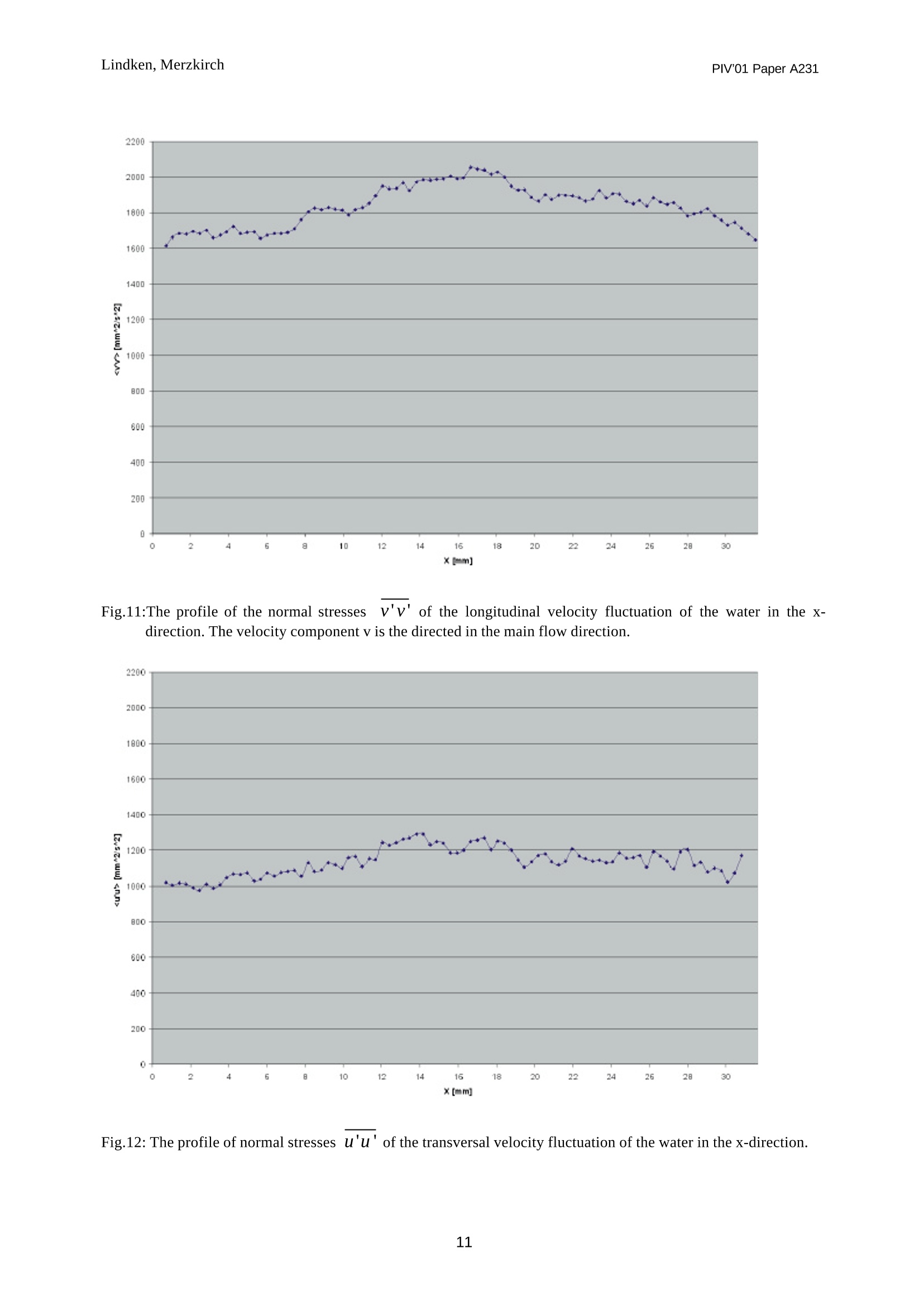
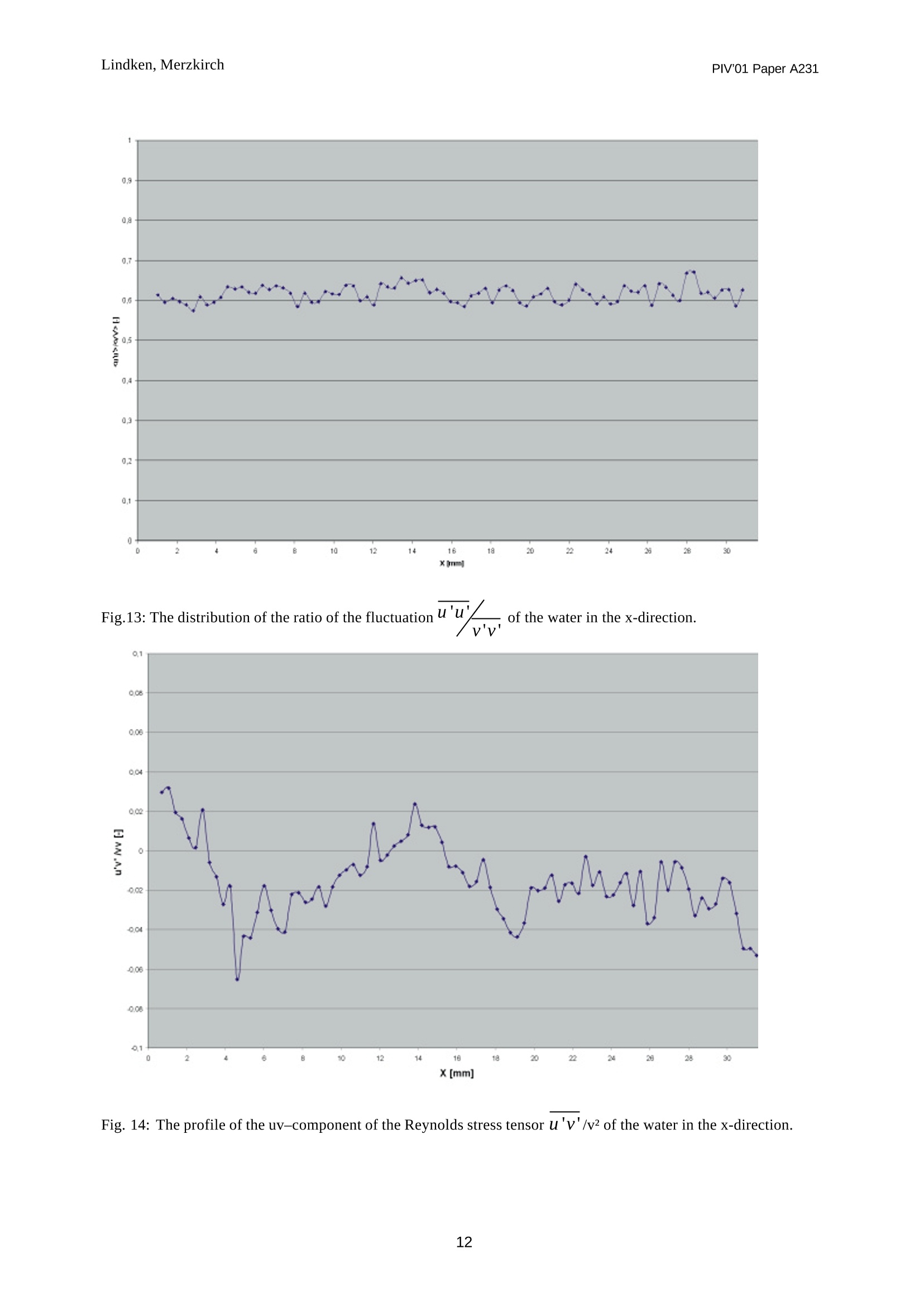
PIV'01 Paper A2314th International Symposium on Particle Image VelocimetryGottingen， Germany， September 17-19， 2001 Lindken， MerzkirchPIV'01 Paper A231 A novel PIV technique for measurements in multi-phase flowsand its application to two-phase bubbly flows R. Lindken， W. Merzkirch Abstract A new experimental procedure for performing simultaneous， phase-separated velocity measurements intwo-phase flows is introduced. Basically this Particle Image Velocimetry (PIV) technique is a combination of thethree most often used PIV techniques in multiphase flows： PIV with fluorescent tracer particles， shadowgraphy andthe digital phase separation with a masking technique. In order to combine the advantages of these multiphase-PIVmethods a new PIV setup was developed. With this setup the velocity distributions of the two phases are measuredsimultaneously with only one b/w camera. This experimental set-up is aimed at providing a means for characterizingthe modification of turbulence in the liquid phase by bubbles， this phenomenon is often called“pseudo-turbulence”(van Wijngaarden， 1998). 1 Introduction In the chemical and biochemical process industry bubble column reactors are used to enforce an intensive masstransfer between gases and liquids. The gas is dispersed in the liquid phase in terms of gas bubbles. The gas bubblesfulfill two tasks. First they allow a very large contact surface even at low gas concentrations； second they induce alocal turbulence that enhances the mixing process. Compared to mechanical mixers the design ofa bubble columnreactor is rather simple， while the fluid mechanical processes are very complex. In recent years there is a largeinterest in the flow behavior of dispersed multiphase flows. Computational fluid Dynamics (CFD) is a widely used tool to investigate the flow behavior in bubbly two-phaseflow. Esmaeeli and Tryggvason (1996， 1999) predicted the flow and the turbulence for clusters of gas bubbles at lowReynolds numbers with Direct Numerical Simulation (DNS). Sokolichin and Eigenberger (1999) simulated a bubblecolumn flow with 3D simulations and the k-e model， but close to the gas outlet they underpredicted the bubblevelocity by a factor of two. A virtual mass force of the fluid carried in the wake was not modeled. Pfleger et al.(1999) simulated a bubble column and came to the conclusion that bubble induced turbulence has to be consideredin their computations. The disagreement between results from numerical simulations show that there is a high demand for experimentalinvestigations. The turbulence field induced by the bubbles rising in the liquid phase is of particular interest.Theofanous and Sullivan (1982) investigated that bubbles produce turbulent energy in turbulent flows. Lance andBataille (1991) showed the influence of a single bubble on turbulence in two-phase flows. They distinguish betweentwo kinds of turbulence： The well-defined grid turbulence and the modification of turbulence by bubbles， calledpseudo-turbulence. Van Wijngaarden (1998) gives a first preliminary explanation of this phenomenon based on therise of non-spherical bubbles described by potential flow theory with the vorticity confined to thin boundary layers，but without tv ovrotretxe xs ]shedding. Ortiz-Villafuerte et al (2000) point out that only with an accurate description of theflow field surrounding the bubble， including the boundary layer of the bubble and its wake， one may producemeaningful results of the potential flow analysis. In bubbly flows with multiple bubbles the existence of pseudo-turbulence in the liquid phase influences themotion of the gas bubbles. There is a two-way coupling of the rising gas bubbles and the pseudo-turbulence in theliquid phase. The bubbles in a swarm rise at a speed different from that of a single bubble rising in stagnant water(for a review see， e.g.， Schliiter and Rabiger 1998). This phenomenon is attributed to the fact that a bubble in aswarm can move in the wake of a preceding bubble (Stewart 1995). Stewart observed that multiple bubbles formclusters or chimney like patterns， often referred to as streaks. ( R . L indken， W. Merzkirch， Fluid Mechanics， University of Essen， 451 1 7 Essen， Germany ) ( c urrent address： Laboratory for Aero and H ydrodynamics， Delft University of Technology， Th e Netherlands ) ( Ralph Lindken， Laboratory for Aero and Hydrodynamics，Delft University of Tech n ology， Leeghwaterstraat 21， 2628 CA Delft， The Netherlands， E-mail： r.lindken@ w bmt.tudelft.nl ) The velocity and turbulence fields in bubbly flows can be surveyed using two-phase PIV. In such studies it isnecessary to separate the information on the velocity of the two phases， dispersed gas bubbles and liquid. There arethree common methods to achieve a separation of the signals originating from the two phases. First there is PIV/LIF that is often used in two-phase spray flows， and that has been applied to bubbly two-phaseflow by Sridhar et al. (1991) and others， too. This PIV technique uses fluorescent tracer particles as markers andrecords with the help of an optical high pass filter the Laser Induced Fluorescence (LIF) signal of the aggregatedtracer particles. A second camera records the light reflected from the gas bubbles. The drawbacks of this method arethat the gas bubbles reflect the LIF signal of the tracers too and cause a severe error in the measurement signal of theliquid flow. The velocity of the gas bubbles is determined from the reflections on the bubbles. These reflectionschange with a speed different from the speed of the bubble due to curvature effects. Furthermore a change of thebubble shape changes the position of the reflection too. The signal for the determination of the bubble velocitycontains all the information of the tracer velocity too. Because the signal of the bubbles is not necessarily strongerthan the signal originating from the tracer， extensive validation of the velocity result is necessary. A typical criterionis the correlation peak width. Another method for PIV in multiphase flow is the separation of the signals originating from the two phases with adigital masking technique. Gui and Merzkirch (1996) describe this method in detail. The digital mask is eithergenerated based on the particle size (Gui et al. 1997)， which assumes that there is a uniform illumination of the gasbubble or with more advanced image processing methods (Song et al 1999， Lindken and Merzkirch 2000). It is veryimportant to notice that the digital mask technique is NOT an image processing technique that separates onetwo-phase flow PIV image in two separate PIV images as often referred by other authors. The digital maskingtechnique is an operator in the PIV evaluation algorithm. It can be added to any cross-correlation， FFT-acceleratedcross-correlation， minimum-quadratic-difference and FFT-accelerated minimum-quadratic-difference algorithm.The advantage of the digital mask technique against an image processing that splits one two-phase-PIV-recording intwo separate recordings with the information of one phase in each recording is that there are no areas withoutinformation of one or the other phase in the recordings. In this way no evaluation errors occur near the interface ofthe two faces. Gui et al. (1997) give a more detailed explanation. Finally a common method in dispersed two-phase flows is shadowgraphy (e.g. Nishino et al.， 2000). A shadowimage of the gas bubbles is recorded on the CCD camera and the velocity distribution of the gas bubbles is evaluatedwith a Particle Tracking Velocimetry (PTV) algorithm. The velocity of the liquid cannot be determined with theshadowgraphy technique. Therefore this technique is often combined with a PIV measurement. Tokuhiro et al(1998) used two cameras facing each other for combined PIV and shadowgraphy measurements on a single bubble. They did not use the information of the position of the bubble for their PIV evaluation， but they deleted all PIVvelocity information at the area of the gas bubble in a post-processing procedure. Lindken and Merzkirch (1999b) used two cameras under a 30° angle， one for PIV measurements and the otherfor shadowgraphy measurements， to measure the velocity with 2D-PIV and the bubble velocity with 3D-PTV. The3D bubble velocity was measured very inaccurately because of the weak signal from the gas bubble in the PIVmeasurement. With this setup they were able to determine the position of the bubbles relative to the 2D-PIV-measurement plane. These methods are well established， but they all have some drawbacks. The PIV/LIF method enhances the signalof the bubbles or tracers， but the signal of the phase that is not evaluated is still causing noise. The digital masktechnique depends on complex pattern recognition procedure to generate the mask. A robust generation of the maskappears not possible up to now. The shadowgraphy and PIV technique with two cameras is the most promisingapproach， but the two cameras are looking on the bubbles under different angles. This causes errors because thebubbles are non-symmetric. When looking at the bubbles under an angle the bubble velocity is measured with alarge error. The new PIV technique combines the advantages of the three above PIV techniques without their disadvantages. 2 The measurement technique 2.1 The principle Fig. 1 shows the principle of the image acquisition with the combined laser light sheet illumination of fluorescenttracer particles and shadow imaging of the gas bubbles. The upper part of the diagram shows the recording of theparticle images， the lower part shows the recording of the bubble images. The boxes describe (from left to right) theillumination procedure， the light originating from the flow， the optical filtering of the signals and the signalsreaching the detector. For the recording of the particle images a frequency doubled， double pulsed Nd：YAG laser at 532 nm wavelengthilluminates a 2D light sheet in the multiphase flow. Fluorescent tracer particles in the flow reflect part of the lightand they emit light at a wavelength of 555-585 nm with an emission peak at 566 nm. The light originating from thetracers reaches an optical high pass filter with a steep transmission edge at 570 nm. The reflected light at 532 nm isblocked， while the fluorescent light passes the filter. The CCD chip detects only light the fluorescent light from thetracers. A double-pulsed high power light emitting diode (LED) array illuminates the multiphase flow for the recordingof the gas bubbles. The LED-array emits light at 675 nm. The flow is back illuminated and the gas bubbles producea shadow. The shadow image with light of the wavelength 675nm passes the optical high pass filter and the shadowimage is recorded on the detector.I. Both information from the tracers and from the bubbles are recorded simultaneously in the same frame of theCCD-chip. They do not interfere with each other， because they are spatially separated in the object field as well as inthe image field. Chapter 2.3 explains how to separate the information. With this set-up light at a wavelength of 532 nm is not reaching the detector. Light with a wavelength of 532nmcontains reflected light from the tracer particles， but also undesired reflections from the gas bubbles. It is regarded asnoise and eliminated by the optical filter. In this manner only the undisturbed signal from the bubbles and the tracersare recorded. Fig.1： Principle of the combined PIV/shadowgraphy experiment 2.2 The Measurement System The PIV part of the experiment is performed with a commercial PIV system， consisting ofa Lumonics double pulseNd：YAG laser with up to 160 mJ per pulse and a LaVision Flowmaster 3 camera with 1000x1280 pixels and 12 bitresolution. A LaVision hardware timing unit controls the PIV system. With the help of the timing unit the PIVmeasurement is triggered to an external event (see chapter 3.2). Additionally the pulsed LED array is integrated in the PIV measurement set-up as shown in figure 2. The pulsedLED array consists of 140 high power diodes with a small emission angle. In front of the LED’s there is a diffuseplate. The LED’s are operated in pulsed mode. This increases the light emission (30 V current for less then 1 ms)，and the moving bubbles do not cause a blurred image. Only with a pulsed illumination the bubble shadow imageshow a uniform intensity in both images of the PIV recording pair. For simultaneous recording of the bubble shadow image and the PIV the LaVision timing unit had to bereprogrammed. Figure 3 shows the timing diagram. The timing of the camera is changed. In the first recording lightis collected for 90 us， compared to 27 us in standard PIV. Within 1 us the data is re moved from the light sensitivepart of the pixels. Then the second recording collects light for 125 ms. At the beginning of the first recording a 8 nslaser pulse illuminates the flow. Simultaneously the pulsed LED array is triggered and the LED’s emit light forabout 12 us. The information from the laser light and the information of the LED illumination are recorded on thefirst frame of the same CCD-chip. After a time interval dt=700us the laser and the LED array are triggered againand the information is recorded in the second frame of the PIV/shadowgraphy recording. LED’s have a behavior totally different from a laser. For that reason some extra effort is necessary to build a LEDillumination system that runs synchronously with the laser. The LED illumination device has a long response timeuntil a current of 30V is built up. For that reason the diodes are set under a permanent current， that is slightly belowthe threshold to start emitting light. When they are triggered only a small increase of the current is necessary. Theresponse time reduces some nanoseconds. Second LED’s keep glowing for several us after the initial trigger. This iscompensated with the sufficiently adjusted length of the recording time (90pus) of the first frame of the PIV recording. Finally the emission of light from LED’s depends considerably on their temperature. With the help of apre-trigger (pulse 0 in figure 3) the LED’s are heated up， so the intensity of light emitted in pulse 1 and pulse 2 isidentical. Fig 2： Set-up and triggering of the combined PIV/shadowgraphy experiment Fig 3： Timing diagram of camera and illumination systems for the combined PIV/shadowgraphy experiment 2.3 The Image Recording Fig. 4 shows a typical PIV/shadowgraphy image. The diagrams on the right and on the bottom show the gray valuedistribution along the horizontal and vertical white lines that are not part of the PIV recording. The diagrams explainthe difference to standard PIV recordings. While for a standard PIV recording the background is as dark as possible(corresponding to low gray values)， for the combined PIV/shadowgraphy measurements the gray value of thebackground is shifted towards higher gray values. In this manner in one b/w image two different kind of informationcan be stored as values higher than the background gray level and as values lower than the background gray value In Fig.4the background has a gray value of about 800 to 1000 counts (of 4096 counts of a 12 bit b/w recording).The tracer particles seen as white dots in the image have gray values sufficiently higher than the background atabout 1500 to 4000 counts. The gas bubbles seen as the large dark areas have a gray value sufficiently lower thanthe background at about 400 to 600 counts. Fig. 4： The combined PIV/shadowgraphy recording shows dark areas， gray background and white spots. The twodiagrams on the right and on the bottom show the gray value distribution along the two white lines in the PIV image.The white lines are not part of the PIV recording. A detailed view of the lower 2000 gray values of a total of 4096gray values (at 12 bit) is shown in the profiles. Dark areas have a gray value lower than background， while the white spots have a gray value higher thanbackground. 2.4 The Image Processing The most challenging part of a PIV measurement in bubbly two-phase flow is the determination of the area that isoccupied by the images of the gas bubbles. PIV methods that did not use a shadowgraphy method to detect the gasbubbles did not succeed completely. Nishino et al. (2000) demonstrated the high accuracy of the size and velocitydetermination with the use ofa shadowgraphy technique. From the PIV/shadowgraphy recording in Fig 4 the area that is occupied by the gas bubbles is evaluated. In a firststep the tracer particles are removed with a median filter. The size of the filter (7x7 px) is sufficiently larger than thetracer particle image. The segmentation is performed with a dynamic gray value threshold. In the histogram of the gray values (Fig. 5)a local minimum determines the threshold. In order to compensate for blur from out-of-focus bubbles the threshold Fig. 5： Histogram of the gray values of the pixels. I therange from 200 to 500 the shadow images of the gasbubbles cause a peak in the gray value distribution. Thepeak in the range from 600 to 1000 gray values is due tothe background illumination. The particle images causevery tiny peaks in the range higher than 1000 gray values.These peaks cannot be resolved in this diagram. n as the minimum + 3 gray values. This localminimum is at a different gray value for everyimage； thus the threshold is evaluated for everyrecording individually. Areaswith agrayvalueelower than thebackground are assigned to the areas occupied bybubbles and areas with a higher gray value areassigned to areas occupied by surrounding liquid.The segmentation gives a rough estimate of thebubble positions. There are several errors in termsof dark areas in the liquid phase from shadows ofthe gas bubbles that are incorrectly assigned to thebubbles. And there are errors from brighter parts ofthe bubbles caused by reflections. These areas areincorrectly assigned to the background. A veryintense post-processing is necessary. Thee post-processing consists of four independent operations.First we fill up the missing areas inside thebubbles. An area is assigned as inside a bubble， if abubble area in at least three directions surrounds it.WiththisCcriterionregions in-between twoneighboringbubblessmaylybe detected too. but these regions will be rejected again with the next criterion. Second the size of the detected area is investigated. Ifthe size exceeds the upper or lower limit of the expected bubble size the detected area is rejected. The next step is toinvestigate the gradient of the gray value distribution. In-focus bubbles have a boundary in a certain gray valuegradient range. Detected areas with a different gray value gradient are rejected. This post-processing algorithmdetects irregular background illumination and the bubble shadows. In the last step we add a 3pixel wide border tothe detected bubble area in order to compensate for blur and reflections on the bubble surfaces. Finally the image is binarized and the binarized image is stored as a digital mask The post-processing algorithms are very expensive in computational time， but with the image processing softwaremore than 99.7 % of the bubble images are automatically detected. Overlapping bubbles are counted as one bubbleThe bubble shape does not influence the accuracy of the image processing.. The prerequisites are a uniformbackground illumination with less than 400 counts difference at a 1000 counts level and a significant gray valuedifference for least 3 quarter of a bubble. 3 Experiment 3.1 Flow Facility The experiments are performed in a transparent cylindrical tank of 200 mm inner diameter filled with de-ionizedwater. In order to minimize distortions in the optical measurements， the test tank is placed inside a water-filledrectangular tank with transparent plane walls. A bubble generator at the bottom of the tank allows the production ofsystems of bubbles with a high reproducibility regarding number and volume of the bubbles. The apparatus consists of seven individual bubble generators that are computer-controlled.Each of the bubblegenerators consists of two electromagnetic valves and an injector. With the two valves a small portion of air isreleased into the tank through an injection system. The injection system consists of a needle in the center of acapillary. The temperature of the water is kept constant at 298 K. A computer-controlled heat exchanger cools the water inthe outer tank to 298 K. The water in the outer tank circulates constantly and there is no temperature gradient in thewater. Through conduction the water in the inner tank is kept constant at 298.3 K. The temperature gradient over theheight of the bubble column is less than 0.1 K. Lindken and Merzkirch (2000) describe the principle and the designof the flow facility in detail. 3.2 PIV measurements The PIV measurements serve to investigate the flow induced in the liquid by clusters of rising bubbles. For thispurpose the water is seeded with fluorescent tracer particles with an average diameter of 10 um (compare Sridhar etal.， 1991). The presence of tracer particles may affect the properties of the air/water interfaces. For bubbles largerthan 3 mm diameter measurements of the bubble rise velocity in "clean”de-ionized water and in water seeded withtracers show differences in the rise velocity in the range of the measurement accuracy. For smaller bubbles Lindkenand Merzkirch (2000) measured a significant drop in the bubble rise velocity measurements. One drawback of optical measurement methods in multiphase slow is the limited optical access. The field of viewis limited through the lens effects of the gas bubbles. The laser light is detoriated and reflected when passing througha gas bubble. In order to measure with little disturbances at a locally high gas void fraction， we do not measure in aconstantly uniform bubble flow. With the help of the computer-controlled bubble generator first a uniform bubbleflow is generated. This flow produces a flow and turbulence field. For the PIV measurements the uniform bubbleflow stops and after a short time interval of 150 ms a system of 14 bubbles with a diameter of 5 to 6 mm rises in theturbulence field generated by the uniform bubble flow. With this set-up we have good optical access to the system of14 bubbles. From former time-resolved measurements (Lindken et al. 2000) the turbulence decay length is estimated to belonger than the distance (3 to 7 cm) between the first field of gas bubbles generating a turbulence field and thesecond system of bubbles rising in this turbulence field. The turbulence decay time is estimated with a bubble size of5.5 mm and velocity fluctuations v’in the wake of about 20 mm/s. The decay time is l/v'=0.28 s. After releasing the system of gas bubbles the bubble generator sends a trigger signal to the PIV system and thePIV measurement starts， when the 14 gas bubbles are in the area of measurement. The mean bubble diameter is5.5 mm. The distance between the bubbles is 1-2 bubble diameters. After one measurement the flow settles for 40seconds， then the bubble generator produces a uniform bubble flow again and the next measurement starts. Weassume that the time delay is sufficient to ensure statically independent measurements. 3.3 PIV evaluation The digital PIV recordings are evaluated with an advanced cross correlation method. The algorithm is extended forthe application in multiphase flow (Gui 1999). Since the two phases， gas bubbles and water， move at differentspeeds， it is necessary to separate in the PIV recordings the signals from the two phases. The idea of applying digitalmasks to separate the signal of the two phases was introduced by Gui and Merzkirch in 1996 so that the flowvelocity of the water and the rise velocity of the bubbles are determined separately but simultaneously. With thisdigital mask technique the water velocity can be measured accurately also in close proximity of the interfaceseparating the two phases (Lindken et al. 1997). We generate the digital masks with the image processing procedure described in chapter 2.4. The digital mask is notan image-processing algorithm. The digital mask is a two-dimensional array of values. The digital mask A(ij) isgenerated such that A(ij)=0 ifa pixel (ij) belongs to the continuos (water) phase A(ij)=1 ifa pixel (i j) belongs to the dispersed (bubble) phase This array (or mask) is combined with the PIV evaluation algorithm as described by Gui (1999). The bubble rise velocities are computed with Particle Tracking Velocimetry (PTV). The particle tracking is notperformed on the original recordings. The original recordings of the gas bubbles contain noise from non-uniformrear illumination and from out of focus bubbles. The image processing procedure in chapter 2.4 determines theshape and position of the bubbles very accurately. The result is a binarized bubble image for each PIV image.The PTV of the gas bubbles is performed on this binarized bubble images. Overlapping bubble images are notseparated with this method. Overlapping gas bubbles are detected as one large gas bubble and only one velocity isevaluated. 4 Results and Discussion Lindken and Merzkirch (2000) have shown the structure of the wake of a system of bubbles rising in water. For theirmeasurements it was necessary to determine the position of the gas bubbles relative to the laser light sheet. In thisway they were able to assign a wake structure to a certain bubble configuration. The measurements in this publication serve to investigate the turbulence structure induced by the gas bubbles in aturbulent flow field. The position of a single bubble is not significant for this measurement. Individual changes inrelative position of shape of gas bubbles average out. The water and the bubble velocity are measured simultaneously when a system of gas bubbles is passing themeasurement plane. The profiles shown in Fig 7 to 14 contain data from 1800 independent measurements. For eachmeasurement we generated a different， but similar systems of bubbles. The average velocity profile of the liquid (water) phase in bubble rise direction (y) is shown in Figure 7. The fluidvelocity is slightly higher in the center of the measurement plane. The center is influenced stronger by the rise of gasbubbles. Fig 8 shows the average velocity profile of the water velocity in thex direction in detail. The distribution ofthe water velocity in x-direction and y-direction shows an accelerated-jet-like behavior of the system of 14 gasbubbles rising in the turbulence field. Water is carried upward with the gas bubbles and the flow spreads to bothsides The rise velocity of the gas bubbles in Fig 9 shows a constant bubble rise velocity. The number density of thedetected gas bubbles (Fig 10) shows that there are more gas bubbles rising in the center of the measurement plane.This indicates that that the jet like profile of the water velocity is not caused by a distribution of the bubble risevelocity， but by the larger number of bubbles rising in the center of the measurement plane. The velocity fluctuations in Fig 11 and 12 show a behavior similar to the profile of the water velocity in bubble rise (y) direction. The normal stresses v'v'and u’u’ are dependent from the position in x-direction. With higher vvelocity the normal stresses rise. The values of the normal stresses are not in the same in the x-and y- direction. The distribution of the ratio of the fluctuations u'u’/v’v' in the x-direction in Fig 13 shows that the fluctuations in the x-direction are about 62% of the fluctuatios in the y-direction. Unlike the other turbulence profiles the profile of the non-dimensional uv-component of the Reynolds stress tensor u’v'/v in the x-direction in Fig. 14 does not show a smooth behaviour. The amount of data seams notsufficient for a accurate determination of the Reynolds stress. Nevertheless it can be shown that the Re-stresses areeffectively zero， which compares well to grid turbulence.. An interpretation of the turbulence data leads us to the conclusion that the two-phase bubbly flow ishomogeneous but anisotropic. The ratio of the longitudinal velocity fluctuations and the transversal velocityfluctuations is close to 2/3. Due to the non-uniform distribution of the gas bubbles the water velocity profile shows the behavior of anaccelerated (e.g. buoyant) jet. The turbulence data show a behavior that is similar to the turbulence in the near fieldbehind a grid. The near field behind a grid (about 1 to 5 mesh widths behind the grid) before the classical 1/z decayof turbulence starts. The near filed behind a grid is characterized by the interaction of multiples of small jetsoriginating from the meshes. While the turbulence in the near region behind a grid is homogeneous in 2 D andanisotropic， the turbulence in a field of bubbles is homogeneous in 3D and anisotropic. Fig. 7： The mean water velocity profile for the velocity v in the x-direction and the mean water velocity profile forthe velocity u. Please note that the v component of the velocity vector is directed in bubble rise (main flow)direction. Fig. 8： A detailed view at the mean water velocity profile for the velocity u in the x-direction. Fig. 9： The average bubble rise velocity in the x-direction. Fig. 10： The histogram of the number of the detected bubbles as a function of the x-direction Fig.11：The profile of the normal stresses1v'v’of the longitudinal velocity fluctuation of the water in the x-direction. The velocity component v is the directed in the main flow direction. Fig.12： The profile of normal stresses u'u’ of the transversal velocity fluctuation of the water in the x-direction. Fig. 13： The distribution of the ratio of the fluctuation‘u'u' of the water in the x-direction. v'v' Fig. 14： The profile of the uv-component of the Reynolds stress tensor U'v'/v’ of the water in the x-direction 5 Summary and Conclusion A novel PIV measurement technique that combines the PIV with fluorescent tracer particles (PIV/LIF)， PIV with adigital masking technique and shadowgraphy has been developed and applied to bubbly two-phase flow. Only oneb/w camera is used to measure the velocity distribution of the continuos (water) and dispersed (bubble) phasesimultaneously. The advantage of this PIV-method is that the signals of the two phases do not disturb each other.They are separated with high very accuracy and the different signals from the two-phase do not cause any noise inthe evaluation. These measurements serve to investigate the turbulence structure induced by the gas bubbles in a turbulent flowfield. From the measurements it can be shown that the turbulence induced by systems of gas bubbles in not isotropicas often premised in computational models. The turbulent fluctuations are significantly higher in the bubble risedirection. The ratio of the longitudinal velocity fluctuations and the transversal velocity fluctuations is about 2/3. These measurements show that the newly developed PIV method for multi-phase flows is able to measurevelocities in two-phase flows with a precision that is high enough to compute turbulent derivations from the data. Amore detailed statement on the turbulence structure in bubbly two-phase flows can only be made after performingseries of measurements with a variation of the gas void fraction and the bubble size. References Esmaeeli A； Tryggvason G (1996) An inverse energy cascade in two-dimensional low Reynolds number bubblyflows. J Fluid Mech 314：315—336 Esmaeeli A； Tryggvason G(1999) Direct numerical simulations of bubbly flows Part 2.Moderate Reynoldsnumber arrays. J Fluid Mech 385：325—358 Gui L (1997) Methodische Untersuchungen zur Auswertung von Aufnahmen der digitalen Particle ImageVelocimetry. Ph.D.-Thesis University of Essen， Shaker Verlag， Aachen， Germany Gui L； Lindken R； Merzkirch W (1997) Phase-separated PIV measurements of the flow around systems ofbubbles rising in water. ASME-FEDSM97-3103， ASME，New York， USA Gui L； Merzkirch W(1996) Phase-separated PIV measurements in two-phase flow by applying a digital masktechnique. ERCOFTAC Bulletin 30： 45—48 Hassan YA； Schmidt WD； Ortiz-Villafuerte J (1998) Investigation of three-dimensional two-phase flowstructure in a bubbly pipe flow. Meas Sci and Technol 9： 309—326 Lance M； Bataille J (1991) Turbulence in the liquid phase of a uniform bubbly air-water flow. J Fluid Mech 222：95—118 ( Lindken R ； Gui L； Merzkirch W (1999) Velocity measurements in multiphase flow by means of particle imagevelocimetry. Chem Eng Technol 22： 202— 2 06 ) ( Lindken R； Merzkirch W (1999) Phase s e parated P IV a nd shadow-image measurements in bubbly two-phase flow. Proc o f t he 8h In t Conf on Laser Anemometry Advances and Applications， Rome ， I， Sept 6-8， 165-171. ) Lindken R； Meyer P； Merzkirch W； Time resolved PIV measurements with systems of bubbles rising in water， Proceedings of the 2000 ASME Fluids Engineering Division Summer Meeting， Boston， USA， ASME，New Yorkpp.FEDSM00-11200. Lindken R； Merzkirch W (2000) Velocity measurements of liquid and gaseous phase for a system of bubblesrising in water. Exp Fluids [Suppl.]： 194—201 Nishino K； Kato H； Torii K (2000) Stereo imaging for simultaneous measurement of size and velocity ofparticles in dispersed two-phase flow. Meas Sci Technol 11， 633-645 Ortiz-Villafuerte J； Schmidl WD； Hassan YA (2000) Three-dimensional ptv study of the surrounding flow andwake of a bubble rising in stagnant liquid. Exp Fluids [Suppl.]：202—210 Pfleger D； Gomes S， Gilbert N； Wagner HG (1999) Hydrodynamic simulations of laboratory scale bubblecolumns fundamental studies of the Eulerian-Eulerian modeling approach， Chem Eng Sci 54：5091--5099 Schliiter M； Rabiger N (1998) Bubble swarm velocity in two-phase flows. HTD-Vol. 361-5， Proceedings of theASME Heat Transfer Division， 5：275—280 Song X； Shen L； Murai Y； Yamamoto F(1999) Separation of particle-bubble images in multiphase flow. Procof the Third International Workshop on PIV'99， Santa Barbara， CA， USA， Sept 16-18， pp. 15—18 Sridhar G； Ran B； Katz J (1991) Implementation of particle image velocimetry to multi-phase flow. Cavitationand Multiphase Flow Forum ASME-FED-Vol.109，205—210， ASME， New York， USA Tassin AL； Nikitopoulos DE (1995) Non-intrusive measurements of bubble size and velocity. Exp Fluids 19：121—132 Theofanous and Sullivan (1982) Turbulence in two-phase dispersed flows J Fluid Mech 116：343—362 Tokuhiro A； Maekawa M； Iizuka K； Hishida K； Maeda M(1998) Turbulent flow past a bubble and anellipsoid using shadow-image and PIV techniques. Int J Multiphase Flow 24， 1383-1406 Van Wijngaarden L (1998)On pseudo turbulence. Theor Comp Fluid Dyn 10， 449—458 Correspondence to：