


方案详情
文
We present an experimental study of the
dynamics of a plume generated from a small heat source in
a high Prandtl number fluid with a strongly temperaturedependent
viscosity. The velocity field was determined
with particle image velocimetry, while the temperature
field was measured using differential interferometry and
thermochromic liquid crystals. The combination of these
different techniques run simultaneously allows us to identify
the different stages of plume development, and to
compare the positions of key-features of the velocity field
(centers of rotation, maximum vorticity locations, stagnation
points) respective to the plume thermal anomaly, for
Prandtl numbers greater than 103. We further show that the
thermal structure of the plume stem is well predicted by the
constant viscosity model of Batchelor (Q J R Met Soc 80:
339–358, 1954) for viscosity ratios up to 50.
1 Introduction
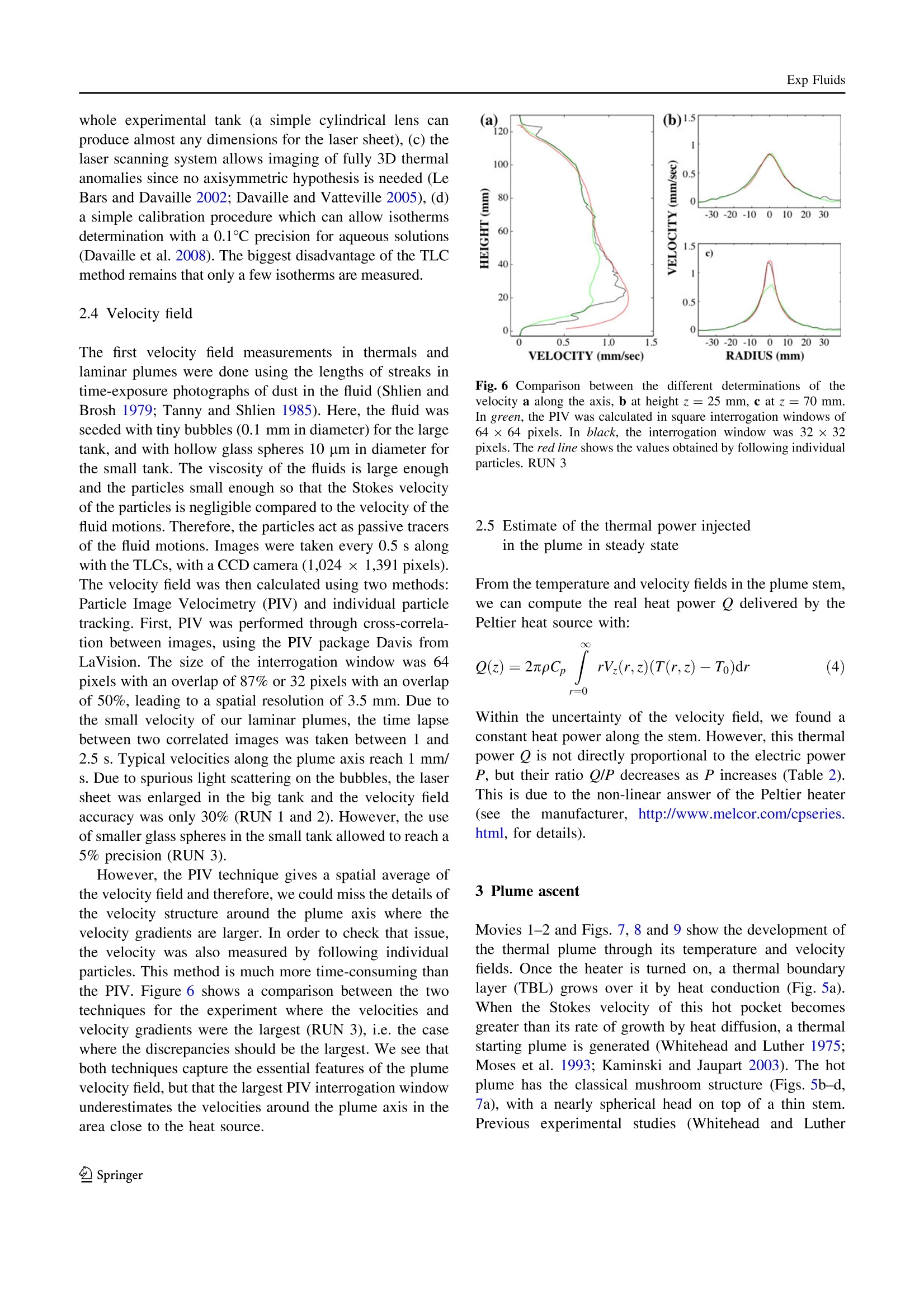
方案详情

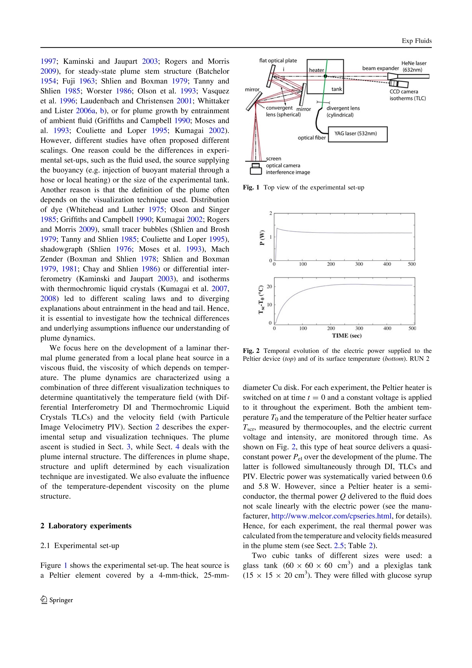
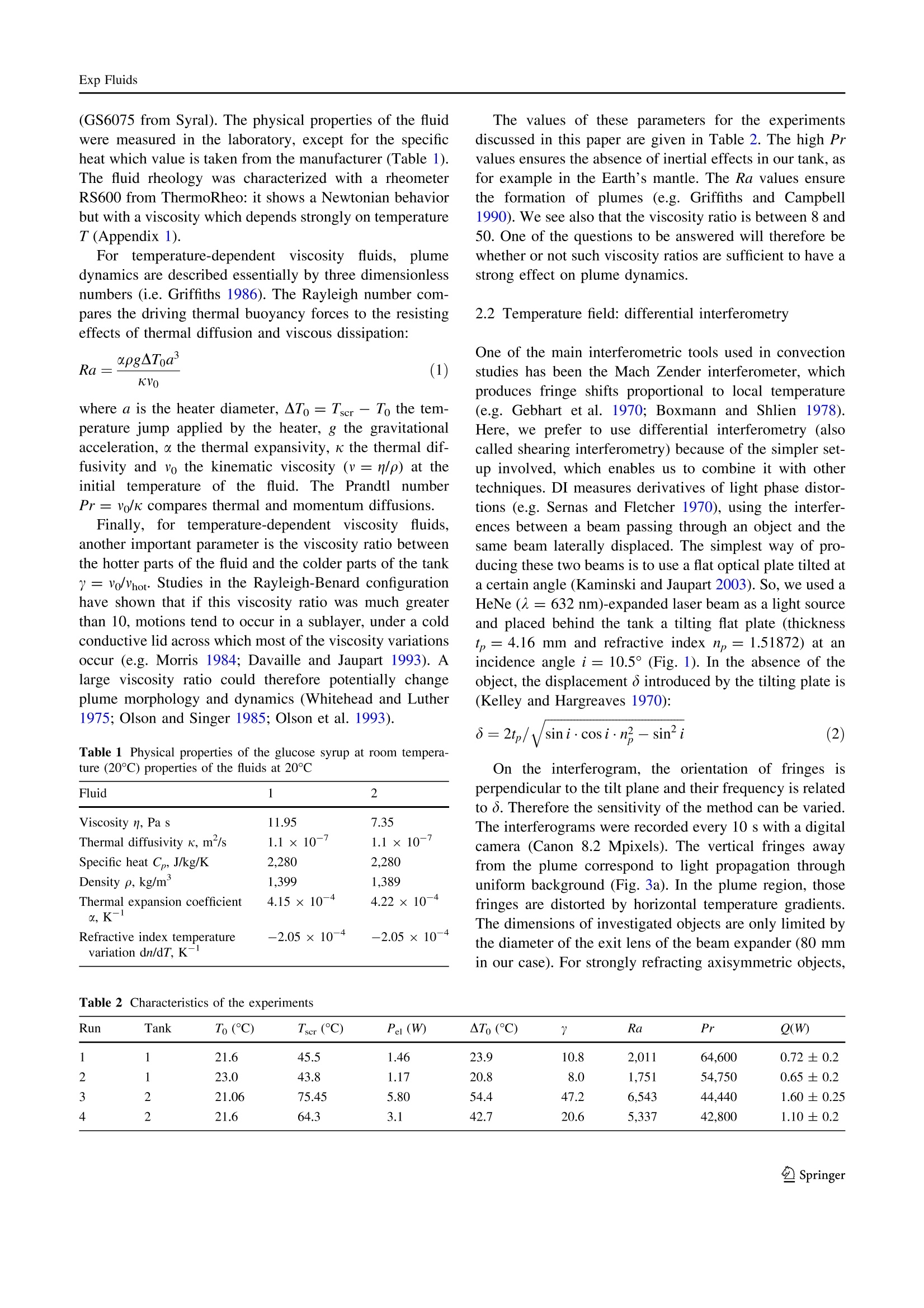
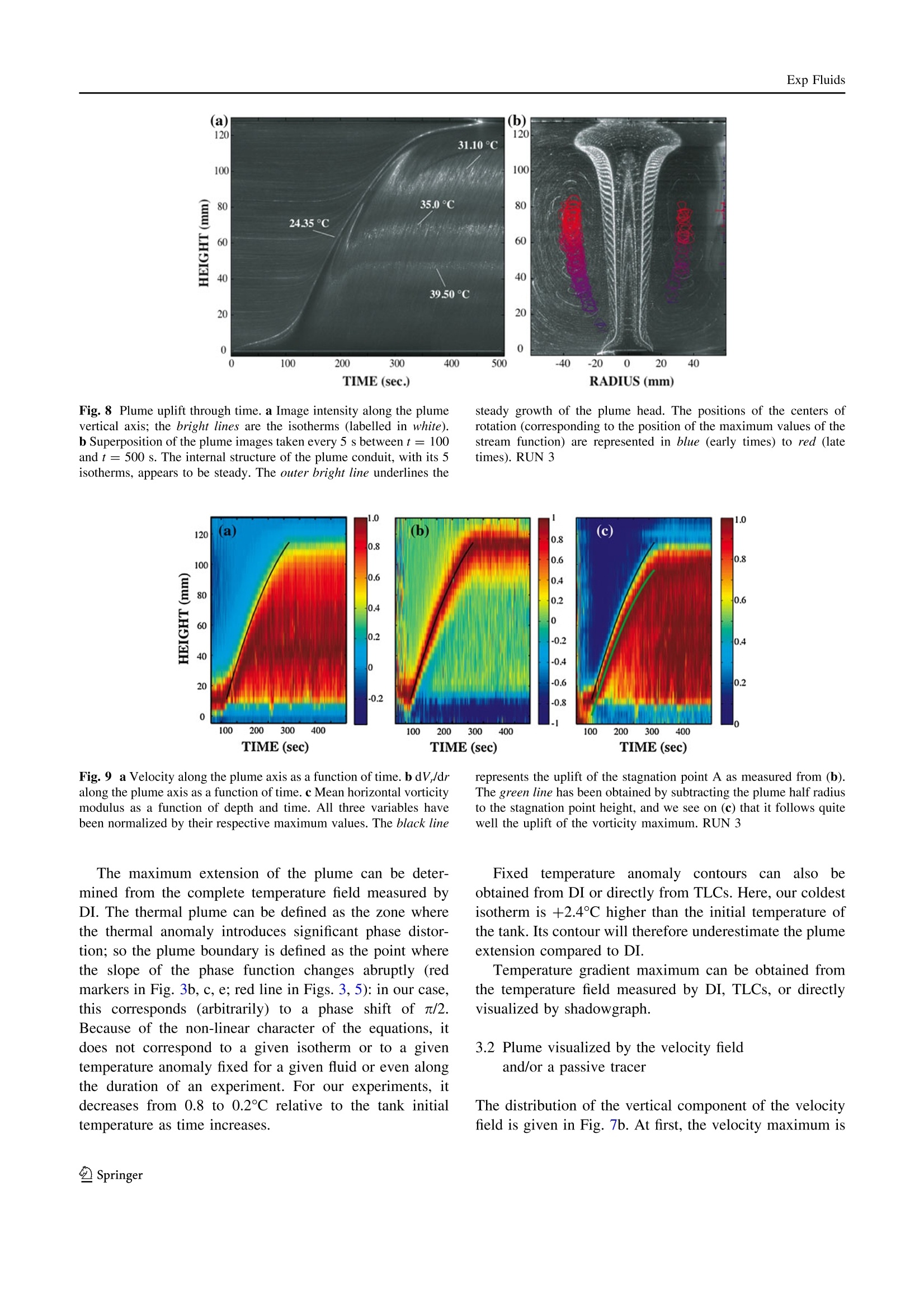
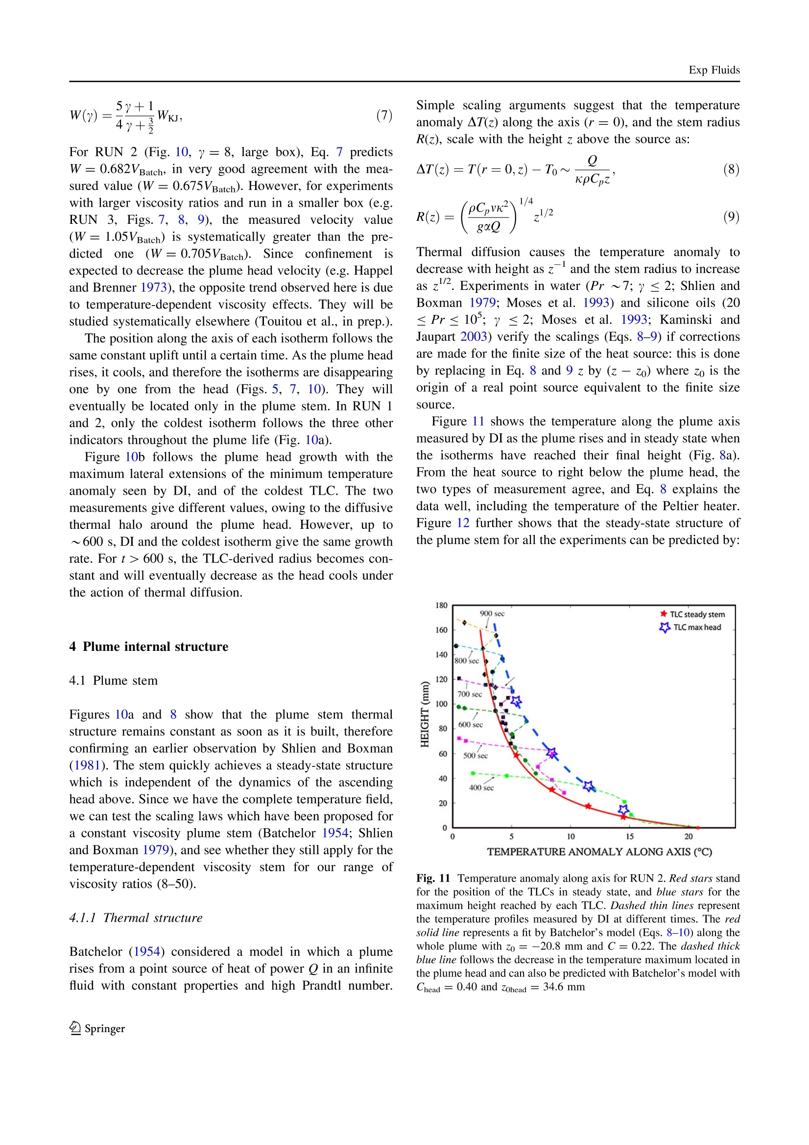
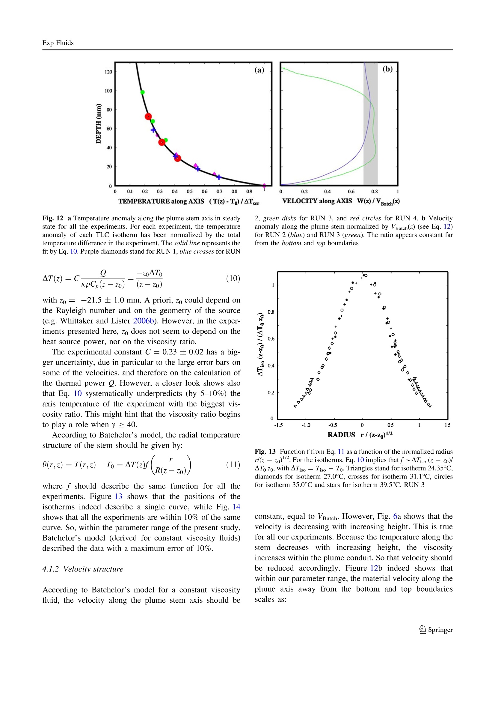
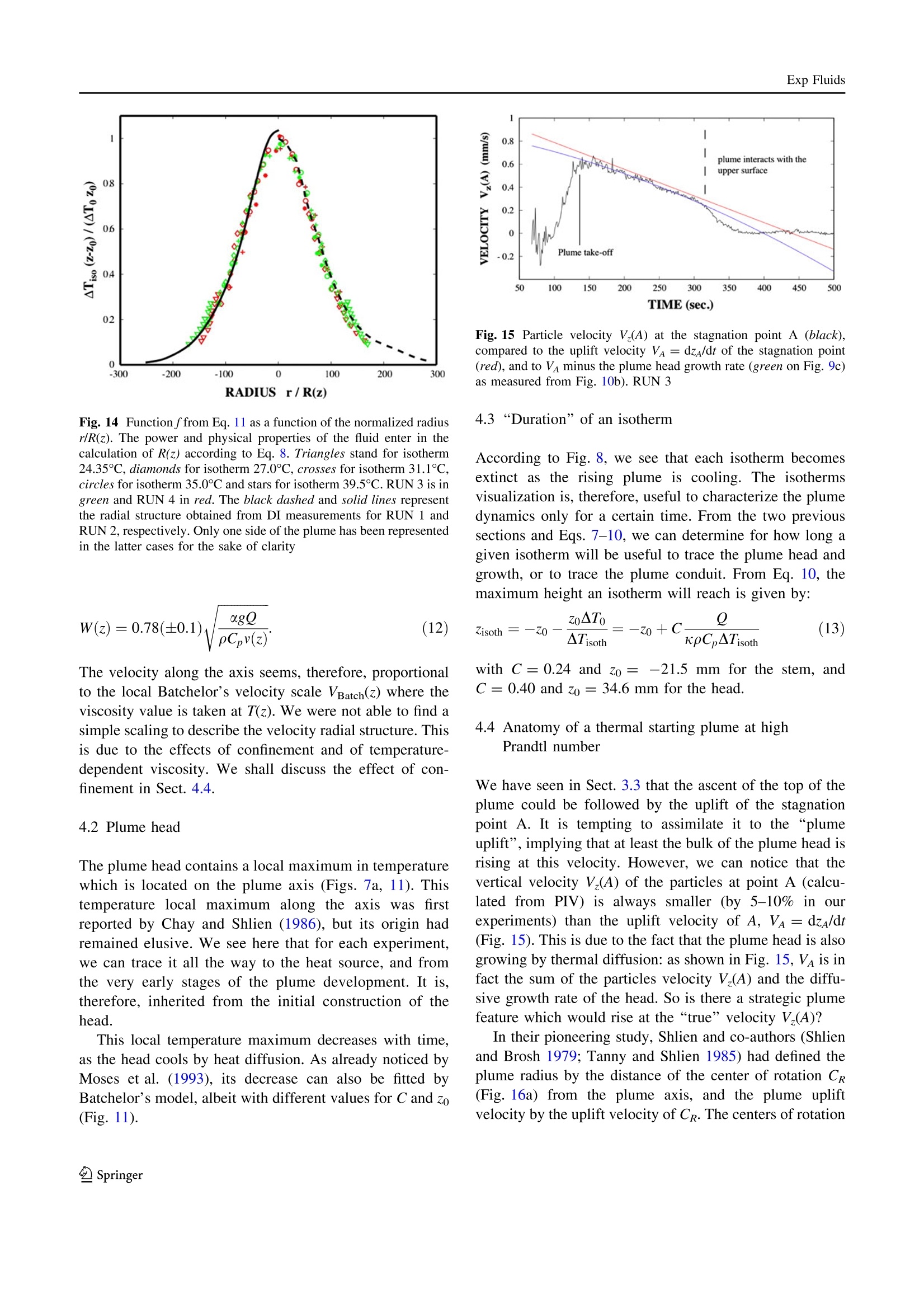
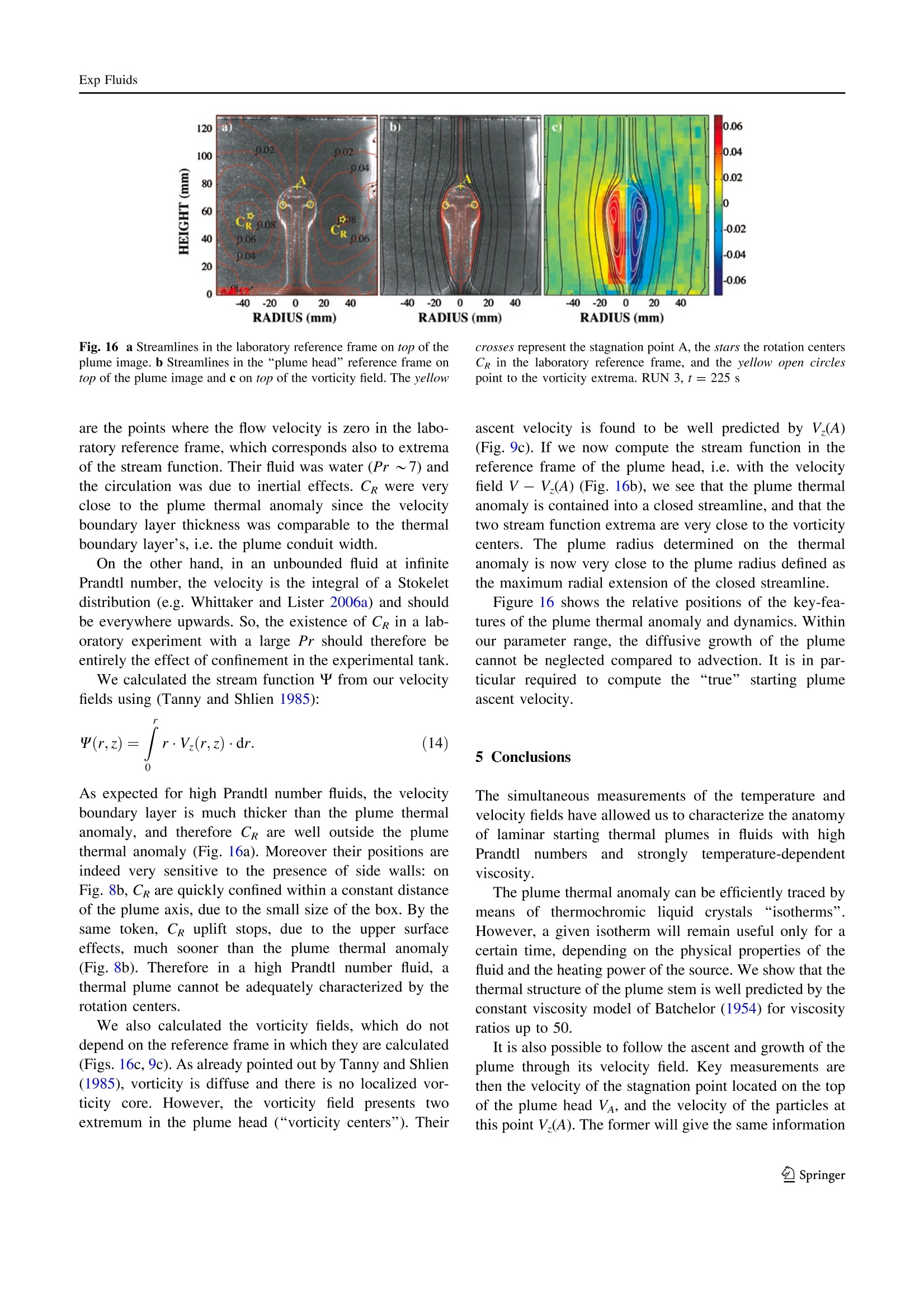
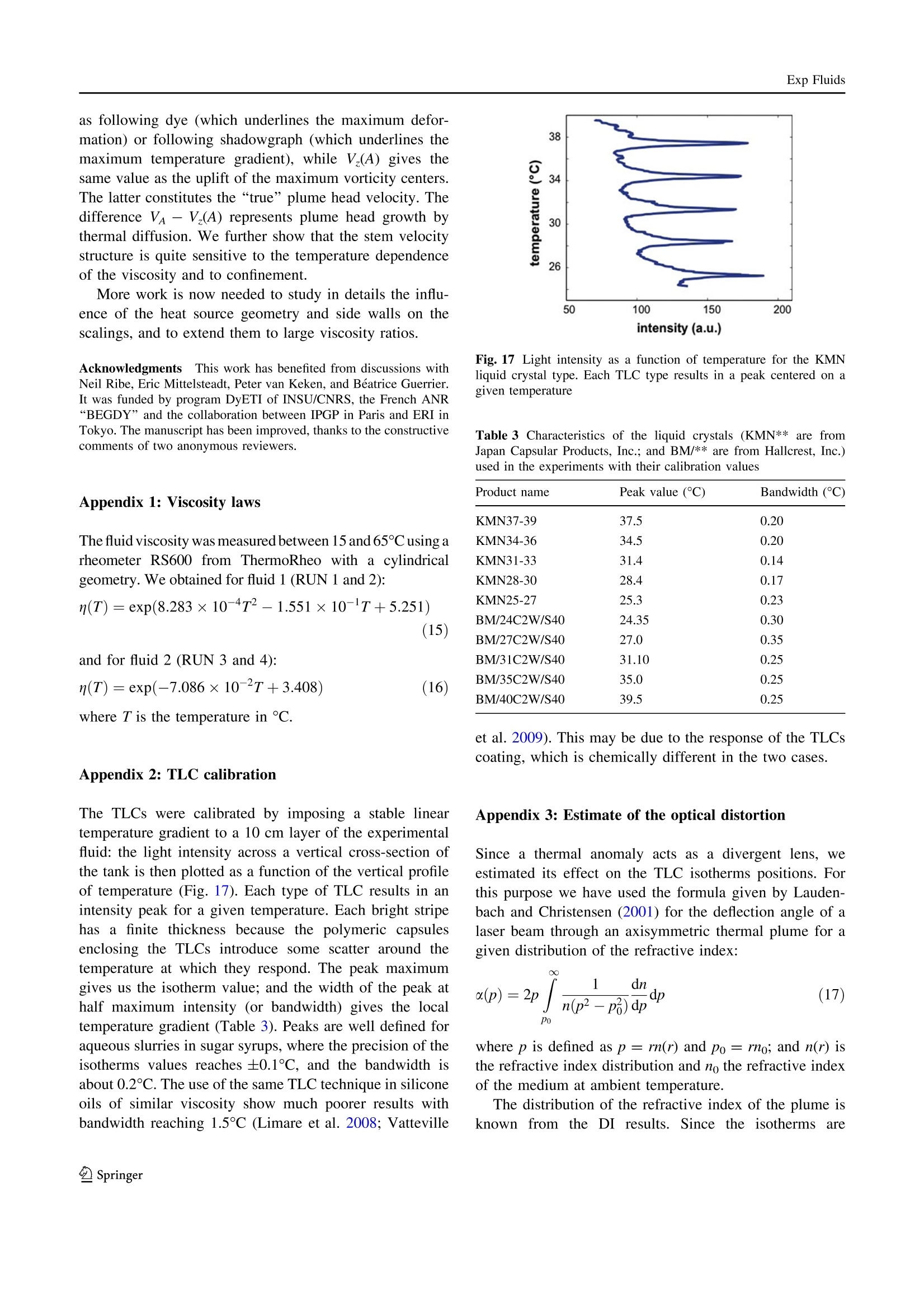
DOI 10.1007/s00348-010-0924-y Exp Fluids Anatomy of a laminar starting thermal plumeat high Prandtl number Anne Davaille· Angela Limare·Floriane Touitou ·Ichiro Kumagai·Judith Vatteville Abstractt We present an (experimental study of thedynamics of a plume generated from a small heat source ina high Prandtl number fluid with a strongly temperature-dependent viscosity. The velocity field was determinedwith particle image velocimetry, while the temperaturefield was measured using differential interferometry andthermochromic liquid crystals. The combination of thesedifferent techniques run simultaneously allows us to iden-tify the different stages of plume development, and tocompare the positions of key-features of the velocity field(centers of rotation, maximum vorticity locations, stagna-tion points) respective to the plume thermal anomaly, for Electronic supplementary materialalThe online version of thisarticle (doi:10.1007/s00348-010-0924-y) contains supplementarymaterial, which is available to authorized users. A. Davaille (区) · F. TouitouLaboratoire FAST, CNRS/UPMC/U-PSud, Bat. 502,Rue du Belvedere, Campus Universitaire,91405 Orsay cedex, Francee-mail: davaille@fast.u-psud.fr A. Limare· I. Kumagai·J. VattevilleDynamique des Fluides Geologiques,IPGP, Univ. Paris 7/CNRS, 4 Place Jussieu,75 252 Paris cedex 05, France Present Address: I. Kumagai Division of Energy and Environmental System, School of Engineering, Hokkaido University, Kita-13, Nishi-8, Kita-ku, Sapporo 060-8628, Japan Present Address: J. Vatteville ( Department of Mechanical Engineering, Un i versity of Thessaly,Leoforos Athinon, Pedion Areos 38834, Volos, Greece ) Prandtl numbers greater than 10’. We further show that thethermal structure of the plume stem is well predicted by theconstant viscosity model of Batchelor (Q J R Met Soc 80:339-358, 1954) for viscosity ratios up to 50. 1 Introduction Plumes are localized regions of buoyant fluid releasedcontinuously through the effect of gravity. They aretherefore, one of the most common feature of thermalconvection, whereby heat transfer occurs by mass trans-port. Plumes are encountered in a number of industrial andnatural situations, such as smoke release from chimneys,waste disposal in oceans, cloud formation processes, andconvection in chemical reactors, magma chambers or in;solid-rock planetary mantles. Plumes can either be turbu-lent, whereby their growth is dominated by turbulententrainment of surrounding material (Morton et al. 1956) o1laminar, in which case their growth is due to thermal dif-fusion, continuous feeding from the source, and laminarentrainment of surrounding material at the rear of a leadingvortical head (Griffiths and Campbell 1990; Kumagai2002) Turner (1962) was the first to study what he called thestarting plume, comprising a steady plume conduit cappedby a large buoyant head. He further suggested that thebuoyancy of the head increases since the head is fed by thestem as a result of the slower upwards motion of the headcompared with the steady stem below it. Since then, mucheffort has been devoted to understand plume dynamics andto provide scalings for plume ascent velocity (Whiteheadand Luther 1975; Shlien 1976; Olson and Singer 1985;.Chay and Shlien 1986; Griffiths and Campbell 1990Moses and al. 1993; Couliette and Loper 1995; van Keken 1997; Kaminski and Jaupart 2003; Rogers and Morris2009), for steady-state plume stem structure (Batchelor1954; Fuji 1963; Shlien and Boxman 1979; Tanny andShlien 1985;, Worster 1986; Olson et al. 1993; Vasquezet al. 1996; Laudenbach and Christensen 2001; Whittakerand Lister 2006a, b), or for plume growth by entrainmentof ambient fluid (Griffiths and Campbell 1990; Moses andal. 1993; Couliette and Loper 1995; Kumagai 2002).However, different studies have often proposed differentscalings. One reason could be the differences in experi-mental set-ups, such as the fluid used, the source supplyingthe buoyancy (e.g. injection of buoyant material through ahose or local heating) or the size of the experimental tank.Another reason is that the definition of the plume oftendepends on the visualization technique used. Distributionof dye (Whitehead and Luther 1975; Olson and Singer1985; Griffiths and Campbell 1990; Kumagai 2002; Rogersand Morris 2009), small tracer bubbles (Shlien and Brosh1979; Tanny and Shlien 1985; Couliette and Loper 1995),shadowgraph (Shlien 1976; Moses et al. 1993), MachZender (Boxman and Shlien 1978; Shlien and Boxman1979, 1981; Chay and Shlien 1986) or differential inter-ferometry (Kaminski and Jaupart 2003), and isothermswith thermochromic liquid crystals (Kumagai et al. 2007,2008) led to different scaling laws and to divergingexplanations about entrainment in the head and tail. Hence,it is essential to investigate how the technical differencesand underlying assumptions influence our understanding ofplume dynamics. We focus here on the development of a laminar ther-mal plume generated from a local plane heat source in aviscous fluid, the viscosity of which depends on temper-ature. The plume dynamics are characterized using acombination of three different visualization techniques todetermine quantitatively the temperature field (with Dif-ferential Interferometry DI and Thermochromic LiquidCrystals TLCs) and the velocity field (with ParticuleImage Velocimetry PIV). Section2 describes the exper-imental setup and visualization techniques. The plumeascent is studied in Sect. 3, while Sect. 4 deals with theplume internal structure. The differences in plume shape,structure and uplift determined by each visualizationtechnique are investigated. We also evaluate the influenceof the temperature-dependent viscosity on the plumestructure. 2 Laboratory experiments 2.1 Experimental set-up Figure 1 shows the experimental set-up. The heat source isa Peltier element covered by a 4-mm-thick, 25-mm- Fig. 1 Top view of the experimental set-up Fig.2 Temporal evolution of the electric power supplied to thePeltier device (top) and of its surface temperature (bottom). RUN 2 Two cubic tanks of different sizesswere used:: aglass tank (60 x60x60 cm’) and a plexiglas tank(15×15×20 cm’). They were filled with glucose syrup (GS6075 from Syral). The physical properties of the fluidwere measured in the laboratory, except for the specificheat which value is taken from the manufacturer (Table 1).The fluid rheology was characterized with a rheometerRS600 from ThermoRheo: it shows a Newtonian behaviorbut with a viscosity which depends strongly on temperatureT(Appendix1). For temperature-dependenttviscosity ffluids, plumedynamics are described essentially by three dimensionlessnumbers (i.e. Griffiths 1986). The Rayleigh number com-pares the driving thermal buoyancy forces to the resistingeffects of thermal diffusion and viscous dissipation: where a is the heater diameter, ATo = Tscr - To the tem-perature jump applied by the heater, g the gravitationalacceleration, a the thermal expansivity, k the thermal dif-fusivity and vo the kinematic viscosity (v=n/p) at theinitial temperature of the fluid. The Prandtl numberPr = vo/k compares thermal and momentum diffusions. Finally, for temperature-dependent viscosity fluids,another important parameter is the viscosity ratio betweenthe hotter parts of the fluid and the colder parts of the tanky= vo/Vhot. Studies in the Rayleigh-Benard configurationhave shown that if this viscosity ratio was much greaterthan 10, motions tend to occur in a sublayer, under a coldconductive lid across which most of the viscosity variationsoccur (e.g. Morris 1984;Davaille and Jaupart 1993). Alarge viscosity ratio could therefore potentially changeplume morphology and dynamics (Whitehead and Luther1975; Olson and Singer 1985; Olson et al. 1993). Table 1 Physical properties of the glucose syrup at room tempera-ture (20°℃) properties of the fluids at 20°℃ Fluid 2 Viscosity n, Pa s 11.95 7.35 Thermal diffusivity k, m²/s 1.1×10- 1.1×10- Specific heat C,, J/kg/K 2.280 2.280 Density p, kg/m’ 1,399 1,389 Thermal expansion coefficient 4.15×10⁻⁴ 4.22x10-+ o, K- Refractive index temperature variation dn/dT, K -2.05×10+ -2.05 x 10+ The values of these parameters for the experimentsdiscussed in this paper are given in Table 2. The high Prvalues ensures the absence of inertial effects in our tank, asfor example in the Earth’s mantle. The Ra values ensurethe formation of plumes (e.g. Griffiths and Campbell1990). We see also that the viscosity ratio is between 8 and. 50. One of the questions to be answered will therefore bewhether or not such viscosity ratios are sufficient to have astrong effect on plume dynamics. 2.2 Temperature field: differential interferometry One of the main interferometric tools used in convectionstudies has been the Mach Zender interferometer, whichproduces fringe shifts proportional to local temperature(e.g. Gebhart et al. 1970; Boxmann and Shlien 1978)Here, we prefer to use differential interferometry (alsccalled shearing interferometry) because of the simpler set-up involved, which enables us to combine it with othertechniques. DI measures derivatives of light phase distor-.tions (e.g. Sernas and Fletcher 1970), using the interfer-ences between a beam passing through an object and thesame beam laterally displaced. The simplest way of pro-ducing these two beams is to use a flat optical plate tilted ata certain angle (Kaminski and Jaupart 2003). So, we used aHeNe (a= 632 nm)-expanded laser beam as a light sourceand placed behind the tank a tilting flat plate (thicknesstp=4.16 mm and refractive index np=1.51872) at anincidence angle i=10.5°(Fig. 1). In the absence of theobject, the displacement introduced by the tilting plate is(Kelley and Hargreaves 1970): On the interferogram, the orientation of fringes isperpendicular to the tilt plane and their frequency is relatedto 8. Therefore the sensitivity of the method can be variedThe interferograms were recorded every 10 s with a digitalcamera (Canon 8.2 Mpixels). The vertical fringes awayfrom the plume correspond to light propagation througuniform background (Fig. 3a). In the plume region, thosefringes are distorted by horizontal temperature gradients.The dimensions of investigated objects are only limited bythe diameter of the exit lens of the beam expander (80 mmin our case). For strongly refracting axisymmetric objects Table 2 Characteristics of the experiments Run Tank To (C) Tscr (C) Pel (W) ATo (℃) Ra Pr Q(W) 1 1 21.6 45.5 1.46 23.9 10.8 2,011 64,600 0.72±0.2 2 1 23.0 43.8 1.17 20.8 8.0 1,751 54,750 0.65±0.2 3 2 21.06 75.45 5.80 54.4 47.2 6,543 44,440 1.60±0.25 4 2 21.6 64.3 3.1 42.7 20.6 5,337 42,800 1.10±0.2 Fig. 3 Plume at t= 475 s forRUN #1. a Left: differentialinterferometry image.The redline shows the contour of thenon-zero thermal anomaly (DIon Fig. 3b, d, e). Right: thebright lines are the isotherms.b Phase h on a horizontal cross-section at 60 mm height.c Phase difference d betweenthe distorted interferogram hand the initial one ho. The blackSh line shows the location of themaximum phase displacementderivative, which wouldcorrespond to a shadowgraphcontour for a purely cylindricalgeometry. d refractive indexdistribution, and e temperaturefield as a function of radius it has been shown (Vest 1975) that accurate results can beobtained only if the interferogram isformedwithappropriate imaging. The convergent lens introduced intothe pathway forms the image of the center plane of theobject on the screen (Fig. 1). The positioning of the lensensures a 1:1 object to image ratio. 2.2.1 Evaluation of the interferogram From the intensity profile of the interferogram along onestraight horizontal line (Fig. 3a), the phase function h iscalculated. The difference in phase between each consec-utive fringe is 2n radians (360°). For the initial interfero-gram, the phase function ho is a straight line as a functionof the pixel number (Fig. 3b). When an object is present,the phase function will be distorted (Fig. 3b), and the dif-ference between the two lines is d(y). The plume axis isdetermined as the point where the two phase functions areintersecting and corresponds to phase difference d(y)= 0(Fig. 3b, c). Then, for an optically thin, axially symmetricobject such as our laminar thermal plume, the refractiveindex distribution introduced by the object can be calcu-lated numerically by simple integration (Pretzler et al.1993) (Fig. 3d): Then,knowing the temperature dependence of the refrac-tiveindex.,theetemperaturefield canbecalculated(Fig.3e). This procedure was applied to all the images. Wechose the incidence angle and the characteristics of the flatplate in order to image accurately most of the plumetemperature anomaly. For distances farther than 3 mmfrom the heat source, the uncertainty is estimated at 0.2°℃ or 2% of the total temperature difference. Closer to the heatsource, the strong temperature gradients render the fringestoo thin to be accurately described. DI has the advantage to give the complete temperaturefield upon inversion of the interferograms. Its disadvan-tages are that: (a) the dimension of the investigated objectdepends on the expansion beam diameter which is limitedby the optics (here only 80 mm diameter), (b) since the testregion is imaged, the position of the thermal anomaly hasto be well determined in advance and (c) it cannot be usedquantitatively for geometries which are neither 2D noraxisymmetric. In the present study, we used DI as a reference to val-idate our TLC method (see next section) and to determinehow the partial image of a plume given by the TLCscompares with the total temperature field given by DI.Disadvantage (a) is the most limiting problem as we cannotimage the plume on its whole ascent. We have thereforeeither focussed on the source region of the plume, keepingthe whole set-up fixed (RUN 1, movie 1), or on the plumecap (RUN 2, movie 2). In the latter, we overcome (a) andfollow the plume cap by rising both the laser and camerasat the same velocity as the plume cap (movie 2). 2.3 Selected isotherms: thermochromic liquid crystals The use of thermochromic liquid crystals (TLC) allowstemperature mapping on a 2D-plane in the fluid flowwithout perturbing it (e.g. Dabiri 2009 for a review, Rheeet al. 1984; Dabiri and Gharib 1991; Willert and Gharib1991). When illuminated by white light, TLC color chan-ges with increasing temperature from invisible to red at lowtemperatures, passes through green and blue to violet andturns invisible again at high temperatures. The total tem-perature range AT accessible with one TLC is between 1 and 40℃. With a high precision color CCD camera, a verystable white light and a precise calibration of the TLC coloragainst true temperature, it is then possible to determine thetemperature field with a 5% precision over AT。 (Fujisawaand Adrian 1999). Since: (a) thermal convection in viscousfluids at high Rayleigh number involves typical tempera-ture heterogeneity of 20-60℃(e.g. Davaille and Limare2007), and (b) we want a temperature precision better than0.2°C, we choose to seed the experimental cell with severaltypes of TLCs, each reflecting light at a different temper-ature, and to illuminate a cross-section of the tank with amonochromatic laser light sheet. Therefore, each type ofTLC is responsible for one bright line, which represents anisotherm (Figs. 5,7a). This method was previously used tostudy two-layer convection (Le Bars and Davaille 2002), Fig. 4 Thermal plume visualized by TLCs (RUN 4). The bright linesare the isotherms. a Vertical cross-section along the plume axis. Thesnapshot is taken with the camera at 90° from the laser sheet. The redarrows indicate the position of the horizontal cross-section of (b) and(c). b Sketch showing the laser sheets positions. c Snapshot takenfrom the top at a 20°from the vertical. It allows seeing the horizontalcross-section of the plume stem as well as the vertical cross sectionabove it Here, the sugar syrup was seeded with five types ofliquid crystals (20-30 um aqueous slurries from JapanCapsular Products, Inc. for the large tank; 40 um aqueousslurries from Hallcrest for the small tank). A vertical cross-section of the experimental tank centered on the plume axisis illuminated by a 532-nm YAG (Coherent VERDI 2W)laser sheet 1 mm thick (Fig.4a). The vertical cross-sectionforms a small angle (~15°) with the section imaged by DI(Fig.1), so that the results from TLC and DI will becomparable only if the plume is axisymmetric. This prop-erty is indeed verified on the horizontal cross-sections ofthe plume (Fig. 4b, c). A black and white CCD camera(LaVision 1,280 × 1,020 pixels) recorded the scatteredlight from the liquid crystals (Fig. 1). Five isotherms wereimaged, with a precision for their peak intensity valueof ±0.1°℃ (see Appendix 2 for details). 2.3.1 Comparison with DI Figure5 shows the TLC images superposed with the cor-responding data for several heights measured by DI. Theagreement between the two methods is good. Even in thehottest part of the plume, the positions of the TLCs iso-therms can be superimposed on the same isotherms deter-mined by DI within 0.1 mm. This is coherent with the factthat optical distortion should be everywhere negligible inour plume parameter range (see Appendix 3). The TLC method has several advantages: (a) directvisualization of some discrete isotherms, (b) a simple setupwith a visualization cross-section which can encompass the Fig. 5 Comparison between theTCL images and thetemperature field calculatedfrom DI for glucose syrup atdifferent moments of the plumeevolution. The points areobtained by intersecting the DItemperature field to the discretevalues of the isotherms. Red lineindicates the DI plumeboundary. RUN 1 E whole experimental tank (a simple cylindrical lens canproduce almost any dimensions for the laser sheet), (c) thelaser scanning system allows imaging of fully 3D thermalanomalies since no axisymmetric hypothesis is needed (LeBars and Davaille 2002; Davaille and Vatteville 2005), (d)a simple calibration procedure which can allow isothermsdetermination with a 0.1C precision for aqueous solutions(Davaille et al. 2008). The biggest disadvantage of the TLCmethod remains that only a few isotherms are measured. 2.4 Velocity field The first velocity field measurements in thermals andlaminar plumes were done using the lengths of streaks intime-exposure photographs of dust in the fluid (Shlien andBrosh 1979; Tanny and Shlien 1985). Here, the fluid wasseeded with tiny bubbles (0.1 mm in diameter) for the largetank, and with hollow glass spheres 10 um in diameter forthe small tank. The viscosity of the fluids is large enoughand the particles small enough so that the Stokes velocityof the particles is negligible compared to the velocity of thefluid motions. Therefore, the particles act as passive tracersof the fluid motions. Images were taken every 0.5 s alongwith the TLCs, with a CCD camera (1,024 × 1,391 pixels).The velocity field was then calculated using two methods:Particle Image Velocimetry (PIV) and individual particletracking. First, PIV was performed through cross-correla-tion between images, using the PIV package Davis fromLaVision. The size of the interrogation window was 64pixels with an overlap of 87% or 32 pixels with an overlapof 50%, leading to a spatial resolution of 3.5 mm. Due tothe small velocity of our laminar plumes, the time lapsebetween two correlated images was taken between 1 and2.5 s. Typical velocities along the plume axis reach 1 mm/s. Due to spurious light scattering on the bubbles, the lasersheet was enlarged in the big tank and the velocity fieldaccuracy was only 30% (RUN 1 and 2). However, the useof smaller glass spheres in the small tank allowed to reach a5% precision (RUN 3). However, the PIV technique gives a spatial average ofthe velocity field and therefore, we could miss the details ofthe velocity structure around the plume axis where thevelocity gradients are larger. In order to check that issue,the velocity was also measured by following individualparticles. This method is much more time-consuming thanthe PIV. Figure 6 shows a comparison between the twotechniques for the experiment where the velocities andvelocity gradients were the largest (RUN 3), i.e. the casewhere the discrepancies should be the largest. We see thatboth techniques capture the essential features of the plumevelocity field, but that the largest PIV interrogation windowunderestimates the velocities around the plume axis in thearea close to the heat source. Fig. 6 Comparison between the different determinations of thevelocity a along the axis, b at height z=25 mm, c at z=70 mm.In green, the PIV was calculated in square interrogation windows of64 × 64 pixels. In black, the interrogation window was 32 ×32pixels. The red line shows the values obtained by following individualparticles. RUN 3 2.5 Estimate of the thermal power injectedin the plume in steady state From the temperature and velocity fields in the plume stem.. we can compute the real heat power g delivered by thePeltier heat source with: Within the uncertainty of the velocity field, we found aconstant heat power along the stem. However, this thermalpower Q is not directly proportional to the electric powerP, but their ratio Q/P decreases as P increases (Table 2)This is due to the non-linear answer of the Peltier heater(see the manufacturer, http://www.melcor.com/cpseries.html, for details). 3 Plume ascent Movies 1-2 and Figs. 7, 8 and 9 show the development ofthe thermal plume through its temperature and velocityfields. Once the heater is turned on, a thermal boundarylayer (TBL) grows over it by heat conduction (Fig.5a)When the Stokes velocity of this hot pocket becomes. greater than its rate of growth by heat diffusion, a thermalstarting plume is generated (Whitehead and Luther 1975;Moses et al. 1993; Kaminski and Jaupart 2003). The hotplume has the classical mushroom structure (Figs. 5b-d,.7a), with a nearly spherical head on top of a thin stemPrevious experimental studies (Whitehead and Luther Fig. 7 Development of theplume through time. RUN 3.a Snapshots at several times.The bright lines are the TLCsisotherms. b Velocity modulus.c Velocity spatial derivativedV,/dr(r, z). The insert showsthe stagnation point above theplume head, where dV,/dr(r, z)should be maximum.d Griddeformation calculated from thevelocity fields. The yellowcrosses show the positions ofthe stagnation point determinedin (c) 60s 125s 155s 190s 230s 305s 1975; Olson and Singer 1985) have shown that this mor-phology always obtained when the plume material was lessviscous than the ambient fluid. This is indeed the case herewhere the hot material has a viscosity much lower than theambient fluid. During the plume rise, the velocity maxi-mum along the plume axis is first located in the plume headbut later descends into the stem where it remains steady(Figs.7b, 9a). To measure plume ascent, we need to consider theplume as an object invading the ambient fluid. Then, there are several ways to identify the plume by its contours and/or averaged properties. 3.1 Plume as a thermal anomaly Since a plume develops because of its buoyant thermalanomaly, the most natural way to describe a plume is byfollowing the thermal anomaly (DI, TLCs) or by followingthe associated temperature gradients (as a shadowgraphwould do). Fig. 8 Plume uplift through time. a Image intensity along the plumevertical axis; the bright lines are the isotherms (labelled in white).b Superposition of the plume images taken every 5 s between t = 100and t = 500 s. The internal structure of the plume conduit, with its 5isotherms, appears to be steady. The outer bright line underlines the steady growth of the plume head. The positions of the centers ofrotation (corresponding to the position of the maximum values of thestream function) are represented in blue (early times) to red (latetimes). RUN 3 n1.0 0.8 0.6 0.4 0.2 Fig. 9 a Velocity along the plume axis as a function of time. b dV,/dralong the plume axis as a function of time. c Mean horizontal vorticitymodulus as a function of depth and time. All three variables havebeen normalized by their respective maximum values. The black line The maximum extension of the plume can be deter-mined from the complete temperature field measured byDI. The thermal plume can be defined as the zone wherethe thermal anomaly introduces significant phase distor-tion; so the plume boundary is defined as the point wherethe slope of the phase function changes abruptly (redmarkers in Fig. 3b, c, e; red line in Figs. 3,5): in our case,this corresponds (arbitrarily) to a phase shift of n/2.Because of the non-linear character of the equations, itdoes not correspond to a given isotherm or to a giventemperature anomaly fixed for a given fluid or even alongthe duration of an experiment. For our experiments, itdecreases from 0.8 to 0.2°C relative to the tank initialtemperature as time increases. represents the uplift of the stagnation point A as measured from (b).The green line has been obtained by subtracting the plume haf radiusto the stagnation point height, and we see on (c) that it follows quitewell the uplift of the vorticity maximum. RUN 3 Fixed temperature anomaly contourscanalso beobtained from DI or directly from TLCs. Here, our coldesisotherm is +2.4℃ higher than the initial temperature ofthe tank. Its contour will therefore underestimate the plumeextension compared to DI. Temperature gradient maximum can be obtained fromthe temperature field measured by DI, TLCs, or directlyvisualized by shadowgraph 3.2 Plume visualized by the velocity field.and/or a passive tracer The distribution of the vertical component of the velocityfield is given in Fig. 7b. At first, the velocity maximum is localized in the plume head; then it moves into the stem. Asimilar behavior was observed in plumes in nearly constantviscosity silicone oils (Vatteville et al. 2009). Following, thevelocity maximum is therefore not a good way to follow theplume uplift. However, previous laboratory experimentsreported that a dye carried by the buoyant axial conduit reachesa stagnation point at the top of the head on the vertical axis(point A on Fig. 7c), from where it spreads laterally into thinlamellae (e.g. Griffiths and Campbell 1990; Kumagai 2002).The existence of this stagnation point in the referential of thegrowing head is also inferred by theoretical studies of isolatedthermals (e.g. Griffiths 1986; Whittaker and Lister 2008).Therefore, an interesting quantity to follow is oV,/Or, whichshould present a local maximum at point A. This is indeed thecase (Figs. 7c, 9b). Moreover, for a stagnation point in anaxisymmetric system, conservation of mass implies that For the plume portrayed in Fig. 7, the ratio between oV/0zand oV,/Or is equal to 1.94±0.32, which, within error,agrees with the theoretical value of 2.0. We also used numerical particles as passive markers (tomimic dye) and advected them using the velocity fields cal-culated by PIV from the laboratory experiment. Initially, theyare regularly dispersed in a 2D numerical grid. At each timestep, they are advected using the velocity field spatially andtemporally interpolated at the position of the particles using afourth-order Runge-Kutta method (van Keken et al. 1997; F.Touitou, G. Brandeis, A. Davaille, Influence of a stronglytemperature-dependent viscosity on mantle plume dynamicsand sampling, in prep.). The top of the plume head is char-acterized by strong horizontal stretching and vertical com-pression of the initial square grid (Fig. 7d). The top of theplume head followed by a passive dye is therefore welldescribed by the point where oV,/or is maximum on thevertical axis. This gives a useful mean to follow the plumehead uplift when only velocity fields are measured. 3.3 Plume ascent and growth seen by the differenttechniques Figure 10a presents a comparison between the differentobservations recorded along the plume axis for a typicalexperiment. In particular, it shows the temporal evolutionof the top edge of the plume cap evaluated by the fourdifferent methods previously described: the top boundaryof the minimum thermal anomaly measured by DI (here-after DI-top), the maximum temperature gradient calcu-lated from the temperature structure (hereafter shadow-top), the height of each TLC isotherm (hereafter TLC-top),and the location of the stagnation point A (hereafter ptA). As expected, DI-top, shadow-top and ptA all describe thesame temporal evolution. Shadow-top and ptA locations are TIME (sec) TIME (sec) Fig. 10 a Plume uplift along vertical axis measured with DI maximalextension (dashed line), TLC isotherms (solid line), stagnation point“A”(reddisks), and maximum temperature gradient (black squares). b Plumegrowth measured by DI anomaly maximum radial extent (dashed line)and the coldest TLC isotherm radial extent (solid line). RUN 2 .undistinguishable within the 1-mm precision of the experi-ments. Away from the top boundary, the plume appears to riseat a constant velocity, in agreement with previous studies (e.gChay and Shlien 1986; Tanny and Shlien 1985; Moses et al.1993; Kaminski and Jaupart 2003; Rogers and Morris 2009)Following Batchelor (1954) and Worster (1986), KaminskiandJaupart (2003) further found that at high Prandtl number ina large box and a nearly constant-viscosity fluid (silicone oil)the “shadow-top”velocity was scaling as: where VBatch= :(Batchelor 1954), and e is solution of. e ln e-2= 1/Pr(Worster 1986). In our experiments, theviscosity depends strongly on temperature and the questionis, therefore, which value of the viscosity is relevant? Now,the ascent velocity of the plume head should be controlledby the viscosity of the most viscous fluid, i.e. the ambienfluid, so that the viscosity in Eq. 6 should be vo. Moreover,the Stokes velocity of a less viscous sphere rising in a moret viscous fluid depends also on the viscosity ratio (e.gWhitehead and Luther 1975; Griffiths 1986), so that thevelocity of our sugar plumes should finally scales as: For RUN 2 (Fig. 10,y=8, large box), Eq. 7 predictsW = 0.682VBatch, in very good agreement with the mea-sured value (W=0.675VBatch). However, for experimentswith larger viscosity ratios and run in a smaller box (e.g.RUN 3, Figs. 7, 8, 9), the measured velocity value(W= 1.05VBatch) is systematically greater than the pre-dicted one((W=0.705VBatch). Since confinement isexpected to decrease the plume head velocity (e.g. Happeland Brenner 1973), the opposite trend observed here is dueto temperature-dependent viscosity effects. They will bestudied systematically elsewhere (Touitou et al., in prep.). The position along the axis of each isotherm follows thesame constant uplift until a certain time. As the plume headrises, it cools, and therefore the isotherms are disappearingone by one from the head (Figs.5, 7,10). They willeventually be located only in the plume stem. In RUN 1and 2, only the coldest isotherm follows the three otherindicators throughout the plume life (Fig. 10a). Figure 10b follows the plume head growth with themaximum lateral extensions of the minimum temperatureanomaly seen by DI, and of the coldest TLC. The twomeasurements give different values, owing to the diffusivethermal halo around the plume head. However, up to~600 s, DI and the coldest isotherm give the same growthrate. For t> 600 s, the TLC-derived radius becomes con-stant and will eventually decrease as the head cools underthe action of thermal diffusion. 4 Plume internal structure 4.1 Plume stem Figures 10a and 8 show that the plume stem thermalstructure remains constant as soon as it is built, thereforeconfirming an earlier observation by Shlien and Boxman(1981). The stem quickly achieves a steady-state structurewhich is independent of the dynamics of the ascendinghead above. Since we have the complete temperature field,we can test the scaling laws which have been proposed fora constant viscosity plume stem (Batchelor 1954; Shlienand Boxman 1979), and see whether they still apply for thetemperature-dependent viscosity stem for our range ofviscosity ratios (8-50). 4.1.1 Thermal structure Batchelor (1954) considered a model in which a plumerises from a point source of heat of power Q in an infinitefluid with constant properties and high Prandtl number. Simple scaling arguments suggest that the temperatureanomaly AT(z) along the axis (r=0), and the stem radiusR(z), scale with the height z above the source as: Thermal diffusion causes tthe temperature anomaly todecrease with height as z- and the stem radius to increaseas z. Experiments in water (Pr ~7;y ≤ 2; Shlien andBoxman 1979; Moses et al. 1993) and silicone oils (2C≤ Pr≤ 10; y ≤ 2; Moses et al. 1993; Kaminski andJaupart 2003) verify the scalings (Eqs. 8-9) if correctionsare made for the finite size of the heat source: this is doneby replacing in Eq. 8 and 9 z by (z -zo) where zo is theorigin of a real point source equivalent to the finite sizesource. Figure 11 shows the temperature along the plume axismeasured by DI as the plume rises and in steady state whenthe isotherms have reached their final height (Fig.8a).From the heat source to right below the plume head, thetwo types of measurement agree, and Eq. 8 explains thedata well, including the temperature of the Peltier heater.Figure 12 further shows that the steady-state structure ofthe plume stem for all the experiments can be predicted by: Fig. 11 Temperature anomaly along axis for RUN 2. Red stars standfor the position of the TLCs in steady state, and blue stars for themaximum height reached by each TLC. Dashed thin lines representthe temperature profiles measured by DI at different times. The redsolid line represents a fit by Batchelor’s model (Eqs. 8-10) along thewhole plume with zo =-20.8 mm and C=0.22. The dashed thickblue line follows the decrease in the temperature maximum located inthe plume head and can also be predicted with Batchelor’s model withChead =0.40 and zohead =34.6 mm Fig. 12 a Temperature anomaly along the plume stem axis in steadystate for all the experiments. For each experiment, the temperatureanomaly of each TLC isotherm has been normalized by the totaltemperature difference in the experiment. The solid line represents thefit by Eq. 10. Purple diamonds stand for RUN 1, blue crosses for RUN 2, green disks for RUN 3, and red circles for RUN 4. b Velocityanomaly along the plume stem normalized by VBatch(z) (see Eq. 12)for RUN 2 (blue) and RUN 3 (green). The ratio appears constant farfrom the bottom and top boundaries with zo=-21.5±1.0 mm. A priori, zo could depend onthe Rayleigh number and on the geometry of the source(e.g. Whittaker and Lister 2006b). However, in the exper-iments presented here, zo does not seem to depend on theheat source power, nor on the viscosity ratio. The experimental constant C= 0.23 ±0.02 has a big-ger uncertainty, due in particular to the large error bars onsome of the velocities, and therefore on the calculation ofthe thermal power Q. However, a closer look shows alsothat Eq. 10 systematically underpredicts (by 5-10%) theaxis temperature of the experiment with the biggest vis-cosity ratio. This might hint that the viscosity ratio beginsto play a role when y 40. According to Batchelor’s model, the radial temperaturestructure of the stem should be given by: Fig. 13 Function f from Eq. 11 as a function of the normalized radiusr/(z- zo)2. For the isotherms, Eq. 10 implies that f~ATiso(z-zo)/ATo zo, with ATiso = Tiso - To. Triangles stand for isotherm 24.35℃,diamonds for isotherm 27.0°C, crosses for isotherm 31.1°C, circlesfor isotherm 35.0°C and stars for isotherm 39.5°C. RUN 3 where f should describe the same function for all theexperiments. Figure 13 shows that the positions of theisotherms indeed describe a single curve, while Fig. 14shows that all the experiments are within 10% of the samecurve. So, within the parameter range of the present study,Batchelor’s model (derived for constant viscosity fluids)described the data with a maximum error of 10%. 4.1.2 Velocity structure According to Batchelor’s model for a constant viscosityfluid, the velocity along the plume stem axis should be constant, equal to VBatch. However, Fig. 6a shows that thevelocity is decreasing with increasing height. This is truefor all our experiments. Because the temperature along thestem decreases with increasing height, the viscosityincreases within the plume conduit. So that velocity shoulcbe reduced accordingly. Figure 12b indeed shows thatwithin our parameter range, the material velocity along theplume axis away from the bottom and top boundariesscales as: Fig. 14 Function ffrom Eq. 11 as a function of the normalized radiusr/R(z). The power and physical properties of the fluid enter in thecalculation of R(z) according to Eq. 8. Triangles stand for isotherm24.35°C, diamonds for isotherm 27.0°C, crosses for isotherm 31.1°C,circles for isotherm 35.0°C and stars for isotherm 39.5°C. RUN 3 is ingreen and RUN 4 in red. The black dashed and solid lines representthe radial structure obtained from DI measurements for RUN 1 andRUN 2, respectively. Only one side of the plume has been representedin the latter cases for the sake of clarity The velocity along the axis seems, therefore, proportionalto the local Batchelor’s velocity scale VBatch(z) where theviscosity value is taken at T(z). We were not able to find asimple scaling to describe the velocity radial structure. Thisis due to the effects of confinement and of temperature-dependent viscosity. We shall discuss the effect of con-finement in Sect. 4.4. 4.2 Plume head The plume head contains a local maximum in temperaturewhich is located on the plume axis (Figs. 7a, 11). Thistemperature local maximum along the axis was firstreported by Chay and Shlien (1986), but its origin hadremained elusive. We see here that for each experiment,we can trace it all the way to the heat source, and fromthe very early stages of the plume development. It is,therefore, inherited from the initial construction of thehead. This local temperature maximum decreases with time,as the head cools by heat diffusion. As already noticed byMoses et al. (1993), its decrease can also be fitted byBatchelor's model, albeit with different values for C and zo(Fig. 11). Fig. 15 Particle velocity V(A) at the stagnation point A (black),compared to the uplift velocity VA = dzA/dt of the stagnation point(red), and to Va minus the plume head growth rate (green on Fig. 9c)as measured from Fig. 10b). RUN 3 4.3“Duration”of an isotherm According to Fig.8, we see that each isotherm becomesextinct as the rising plume is cooling. The isothermsvisualization is, therefore, useful to characterize the plumedynamics only for a certain time. From the two previoussections and Eqs. 7-10, we can determine for how long agiven isotherm will be useful to trace the plume head andgrowth, or to trace the plume conduit. From Eq. 10, themaximum height an isotherm will reach is given by: with C=0.24 and zo=-21.5 mm for the stem, andC=0.40 and zo =34.6 mm for the head. 4.4 Anatomy of a thermal starting plume at highPrandtl number We have seen in Sect. 3.3 that the ascent of the top of theplume could be followed by the uplift of the stagnationpoint A. It is tempting to assimilate it to the ‘“plumeuplift”, implying that at least the bulk of the plume head isrising at this velocity. However, we can notice that thevertical velocity V(A) of the particles at point A (calcu-lated from PIV) is always smaller (by 5-10% in ourexperiments) than the uplift velocity of A, VA= dzA/dt(Fig. 15). This is due to the fact that the plume head is alscgrowing by thermal diffusion: as shown in Fig. 15, V is infact the sum of the particles velocity V(A) and the diffu-sive growth rate of the head. So is there a strategic plumefeature which would rise at the “true”velocity V(A)? In their pioneering study, Shlien and co-authors (Shlienand Brosh 1979; Tanny and Shlien 1985) had defined theplume radius by the distance of the center of rotation Cr(Fig. 16a) from the plume axis, and the plume upliftvelocity by the uplift velocity of Cr. The centers of rotation are the points where the flow velocity is zero in the labo-ratory reference frame, which corresponds also to extremaof the stream function. Their fluid was water (Pr ~7) andthe circulation was due to inertial effects. Cr were veryclose to the plume thermal anomaly since the velocityboundary layer thickness was comparable to the thermalboundary layer’s, i.e. the plume conduit width. On the other hand, in an unbounded fluid at infinitePrandtl number, the velocity is the integral of a Stokeletdistribution (e.g. Whittaker and Lister 2006a) and shouldbe everywhere upwards. So, the existence of CR in a lab-oratory experiment with a large Pr should therefore beentirely the effect of confinement in the experimental tank. We calculated the stream function Y from our velocityfields using (Tanny and Shlien 1985): As expected for high Prandtl number fluids, the velocityboundary layer is much thicker than the plume thermalanomaly, and therefore Cr are well outside the plumethermal anomaly (Fig. 16a). Moreover their positions areindeed very sensitive to the presence of side walls: onFig. 8b, Cr are quickly confined within a constant distanceof the plume axis, due to the small size of the box. By thesame token, Cr uplift stops, due to the upper surfaceeffects, much sooner than the plume thermal anomaly(Fig. 8b). Therefore in a high Prandtl number fluid, athermal plume cannot be adequately characterized by therotation centers We also calculated the vorticity fields, which do notdepend on the reference frame in which they are calculated(Figs. 16c,9c). As already pointed out by Tanny and Shlien(1985), vorticity is diffuse and there is no localized vor-ticity core. However, the vorticity field presents twoextremum in the plume head (“vorticity centers"). Their crosses represent the stagnation point A, the stars the rotation centersCe in the laboratory reference frame, and the yellow open circles:point to the vorticity extrema. RUN 3,t=225 s ascent velocity is found to be well predicted by V(A)(Fig. 9c). If we now compute the stream function in thereference frame of the plume head, i.e. with the velocityfield V - V(A) (Fig. 16b), we see that the plume thermalanomaly is contained into a closed streamline, and that thetwo stream function extrema are very close to the vorticitycenters. The plume radius determined on the thermalanomaly is now very close to the plume radius defined asthe maximum radial extension of the closed streamline. Figure 16 shows the relative positions of the key-fea-tures of the plume thermal anomaly and dynamics.Withinour parameter range, the diffusive growth of the plumecannot be neglected compared to advection. It is in par-ticular required to compute the “true”starting plumeascent velocity. 5 Conclusions The simultaneous measurements of the temperature andvelocity fields have allowed us to characterize the anatomyof laminar starting thermal plumes in fluids with highPrandtl11numbers andstronglyy temperature-dependentviscosity. The plume thermal anomaly can be efficiently traced bymeans of thermochromic liquid crystals6“6isotherms”However, a given isotherm will remain useful only for acertain time, depending on the physical properties of thefluid and the heating power of the source. We show that thethermal structure of the plume stem is well predicted by theconstant viscosity model of Batchelor (1954) for viscosityratios up to 50. It is also possible to follow the ascent and growth of theplume through its velocity field. Key measurements arethen the velocity of the stagnation point located on the topof the plume head VA, and the velocity of the particles atthis point V(A). The former will give the same information as following dye (which underlines the maximum defor-mation) or following shadowgraph (which underlines themaximum temperature gradient), while V(A) gives thesame value as the uplift of the maximum vorticity centers.The latter constitutes the “true" plume head velocity. Thedifference VA - V(A) represents plume head growth bythermal diffusion. We further show that the stem velocitystructure is quite sensitive to the temperature dependenceof the viscosity and to confinement. More work is now needed to study in details the influ-ence of the heat source geometry and side walls on thescalings, and to extend them to large viscosity ratios. AcknowledgmentsThis work has benefited from discussions withNeil Ribe, Eric Mittelsteadt, Peter van Keken, and Beatrice Guerrier.It was funded by program DyETI of INSU/CNRS, the French ANR“BEGDY” and the collaboration between IPGP in Paris and ERI inTokyo. The manuscript has been improved, thanks to the constructivecomments of two anonymous reviewers. Appendix 1: Viscosity laws The fluid viscosity was measured between 15 and65°Cusing arheometer RS600 from ThermoRheo with a cylindricalgeometry. We obtained for fluid 1 (RUN 1 and 2): and for fluid 2 (RUN 3 and 4): where T is the temperature in °C. Appendix 2: TLC calibration The TLCs were calibrated by imposing a stable lineartemperature gradient to a 10 cm layer of the experimentalfluid: the light intensity across a vertical cross-section ofthe tank is then plotted as a function of the vertical profileof temperature (Fig. 17). Each type of TLC results in anintensity peak for a given temperature. Each bright stripehas a finite thickness because the polymeric capsulesenclosing the TLCs introduce some scatter around thetemperature at which they respond. The peak maximumgives us the isotherm value; and the width of the peak athalf maximum intensity (or bandwidth) gives the localtemperature gradient (Table 3). Peaks are well defined foraqueous slurries in sugar syrups, where the precision of theisotherms values reaches ±0.1°C, and the bandwidth isabout 0.2°C. The use of the same TLC technique in siliconeoils of similar viscosity show much poorer results withbandwidth reaching 1.5℃ (Limare et al. 2008; Vatteville Fig. 17 Light intensity as a function of temperature for the KMNliquid crystal type. Each TLC type results in a peak centered on agiven temperature Table 3 Characteristics of the liquid crystals (KMN** are fromJapan Capsular Products, Inc.; and BM/** are from Hallcrest, Inc.)used in the experiments with their calibration values Product name Peak value (C) Bandwidth (C) KMN37-39 37.5 0.20 KMN34-36 34.5 0.20 KMN31-33 31.4 0.14 KMN28-30 28.4 0.17 KMN25-27 25.3 0.23 BM/24C2W/S40 24.35 0.30 BM/27C2W/S40 27.0 0.35 BM/31C2W/S40 31.10 0.25 BM/35C2W/S40 35.0 0.25 BM/40C2W/S40 39.5 0.25 et al. 2009). This may be due to the response of the TLCscoating, which is chemically different in the two cases. Appendix 3: Estimate of the optical distortion Since a thermal anomaly acts as a divergent lens, weestimated its effect on the TLC isotherms positions. Foithis purpose we have used the formula given by Lauden-bach and Christensen (2001) for the deflection angle of alaser beam through an axisymmetric thermal plume for agiven distribution of the refractive index: where p is defined as p= rn(r) and po = rno;and n(r) isthe refractive index distribution and no the refractive indexof the medium at ambient temperature. The distribution of the refractive index of the plume isknown from the DI results. Since the isotherms are Fig. 18 Optical distortion induced by the thermal anomaly on theTLC images: a horizontal temperature profiles, b deflection angle,and c shift on the images, as a function of the radial coordinate visualized in a plane passing through the center of theplume, we therefore considered that the deflection angle ofthe scattered light from the isotherms was equal to half ofthe total deflection angle of a virtual beam passing throughthe entire plume. In our case, this angle remains smallerthan 10-3 radian. This implies that the associated shift inlocation of a given isotherm would remain smaller than5×10- mm (Fig. 18). References Batchelor GK (1954) Heat convection and buoyancy effects in fluids.Q J R Met Soc 80: 339-358 Boxman RL, Shlien DJ (1978) Interferometric measurement tech-nique for the temperature field of axisymmetric buoyantphenomena. Appl Opt 17:2788-2793 Chay A, Shlien DJ (1986) Scalar field measurements of a laminarstarting plume cap using digital processing of interferograms.Phys Fluids 29: 2358-2366 Couliette DL, Loper DE (1995) Experimental, numerical andanalytical models of mantle starting plumes. Phys Earth PlanetInter 92: 143-167 Dabiri D, Gharib M (1991) Digital particle image thermometry: themethod and implementation. Exp Fluids 11: 77-86 Dabiri D (2009) Digital liquid crystal particle thermometry/veloci-metry (DLCPT/V)-a review. Exp Fluids 46(2): 191-241 Davaille A. Jaupart C (1993) Transient high-Rayleigh numberthermal convection with large viscosity variations. J Fluid Mech253:141-166 Davaille A. VattevilleJ (2005) On the transient nature of mantleplumes. Geophys Res Lett 32: L14309 doi:10.1029/2005GL023029 Davaille A, Limare A (2007) Laboratory studies on mantle convec-tion. In: Bercovici D, Schubert G (eds) Treatise of geophysics.Elsevier, Amsterdam, pp 89-165 Davaille A, Androvandi S, Vatteville J, Limare A, Vidal V, Lebars M(2008) Thermal boundary layer instabilities in viscous fluids. In:ISFV13-13th International symposium on flow visualization,July 1-4, 2008,Nice, France,p 12, available at http://www.ipgp.fr/~limare/317.pdf Fuji T (1963) Theory of the steady laminar natural convection above ahorizontal line heat source and a point heat source. Int J HeatMass Transf 6: 597-606 Fujisawa N, Adrian R (1999) Three-dimensional temperature mea-surement in turbulent thermal convection by extended rangescanning liquid crystal thermometry. J Vis 1:355-364 Gebhart B, Pera L, Schorr WA (1970) Steady laminar naturalconvection plumes above a horizontal line heat source. Int J HeatMass Tranf 13: 161-171 Griffiths RW (1986) Thermals in extremely viscous fluids, includingthe effects of temperature dependent viscosity. J Fluid Mech166:115-138 Griffiths RW, Campbell IH (1990) Stirring and structure in mantlestarting plumes. Earth Planet Sci Lett 99: 66-78 Happel J, Brenner H (1973) Low Reynolds number hydrodynamics.Noordhoff, Leyden Kaminski E, Jaupart C (2003) Laminar starting plumes in high-Prandtl-number fluids. J Fluid Mech 478:287-298 Kumagai I (2002) On the anatomy of mantle plumes: effect of theviscosity ratio on entrainment and stirring. Earth Planet Sci Lett198:211-224 Kumagai I, Davaille A, Kurita K (2007) On the fate of thermalplumes at density interface, earth planet. Sci Lett 254: 180-193 Kumagai I, Davaille A, Kurita K, Stutzmann E (2008) Mantle plumes:thin, fat, successful, or failing? Constraints to explain hot spotvolcanism through time and space, Geophys. Res Lett 35:L16301 http://www.dx.doi.org/10.1029/2008GL035079 Kelley JG, Hargreaves RA (1970) A rugged inexpensive shearinginterferometer Appl Opt 9: 948-952 Laudenbach N, Christensen UR (2001) An optical method formeasuring temperature in laboratory models of mantle plumes.Geophys J Int 145:528-534 Le Bars M, Davaille A (2002) Stability of thermal convection in twosuperimposed miscible viscous fluids. J Fluid Mech 471:339-363 ( Morris S, C anright D R (1984) A boundary-layer ana l ysis of Be n ard convection with strongly t e mperature-dependent viscosity. PhysEarth Planet Inter 36 : 355-373 ) ( Morton BR, T a y l or GI, Turner JS (1956) Tu r bulent gr a vitationalconvection from m aintained a nd instantaneous sources. Proc RSoc Lond A 234:1-23 ) ( Moses E, Zocchi G , Libchaber A ( 1 993) A n experimental s t udy oflaminar plumes. J Fluid Mech 251: 581-601 ) ( Olson P , Singer H (1985) Creeping plumes. J Fluid Mech 158: 5 11 - 531 ) ( Olson P, S chubert G , Anderson C (1993) Structure o f axisymmetric p lumes. J Geophys Res 98: 6829-6844 ) ( Pretzler G, Jager H , Neger T ( 1993) High-accuracy differentialinterferometry for t he i nvestigation o f p hase objects. Meas SciTechnol 4: 649-658 ) ( Rhee H, K o seff J , S t reet R (1984) Flow vi s ualization o f a recirculating flow by rheoscopic a nd liquid c rystal techniques. Exp F luids 2: 57-64 ) ( Rogers MC, Morris SW (2009) Natural v e rsus forced c onvection i nlaminar starting plumes. Phys Fluids 21: 0 8 3601 ) ( Sernas V, Fletcher LS ( 1970) A schlieren interferometer method for h eat t ransfer studies . J Hea t Transf 92: 202-204 ) ( Shlien DJ (1976) Some laminar thermal and plume experiments. PhysFluids 19: 1089-1098 ) ( Shlien DJ, Boxman R L (1979) Temperature field m e asurement of an axisymmetric l aminar plume. Phys Fluids 22(4):631-634 ) ( Shlien D J, Brosh A (1979) Velocity field measurements of a laminarthermal. Phys Fluids 22: 1044-1053 ) ( Shlien DJ, Boxman RL (1981) L aminar st a rting plume t e mperature f ield measurement. Intl J Heat Mass Transf 24: 919-930 ) ( Tanny J, Shlien DJ(1985) Velocity field measurements of a laminarstarting plume. Phys Fluids 28: 1027-1032 ) Turner JS (1962) The starting plume in neutral surroundings. J FluidMech 13:356-368 ( van K eken P E (1997) Evolution of starting mantle pl u mes: acomparison b etween l a boratory and n u merical m o dels. E a rth Planet Sci Lett 148: 1-14 ) ( van K eken P, King S, Schmeling H, Christensen U , N eumeister D, Doin M-P ( 1 997) A comparison of methods fo r the m o deling of thermochemical convection. JGeophys Res 102(B10): 2 2477- 22495 ) ( Vasquez PA, P e rez A T , Castellanos A (1 9 96) Thermal and ele c tro-hydrodynamics plumes. A comparative study. Phys Fluids 8 : 2091-2096 ) ( Vest C M (1975) In t erferometry of st r ongly refracting axisymmetric p hase objects. Appl Opt 14:1601-1606 ) ( Whitehead J A , L u ther D S (1 9 75) Dynamics of laboratory diapir andplume models. J Geophys Res 80: 7 05-717 ) Whittaker RJ, Lister JR (2006a) Steady axisymmetric creepingplumes above a planar boundary. Part I: a point source. J FluidMech 567: 361-378 ( Whittaker RJ, L ister JR (2006b) S t eady ax i symmetric cre e ping p lumes above a p l anar b o undary. Part I I : a d istributed source.J Fluid Mech 567:379-397 ) ( Whittaker R J, L ister J R ( 2008) The s e lf-similar r ise of a b uoyant thermal i n v ery viscous flow. J Fluid Mech 606: 295-324 ) ( Willert C, G harib M (1991) Digital p article image thermometry. ExpFluids 10: 181-193 ) ( Worster MG (1986) The axisymmetric laminar p lumes: asymptoticsolution for large Prandtl number. Stud Appl Math 75 : 139-152 ) Springer
确定


还剩14页未读,是否继续阅读?

产品配置单


北京欧兰科技发展有限公司为您提供《热卷流中高普朗特数薄层热卷流发展的剖析检测方案(粒子图像测速)》,该方案主要用于其他中高普朗特数薄层热卷流发展的剖析检测,参考标准--,《热卷流中高普朗特数薄层热卷流发展的剖析检测方案(粒子图像测速)》用到的仪器有德国LaVision PIV/PLIF粒子成像测速场仪、Imager sCMOS PIV相机、PLIF平面激光诱导荧光火焰燃烧检测系统
推荐专场


相关方案
更多
该厂商其他方案
更多