空气流体中速度矢量场检测方案(粒子图像测速)

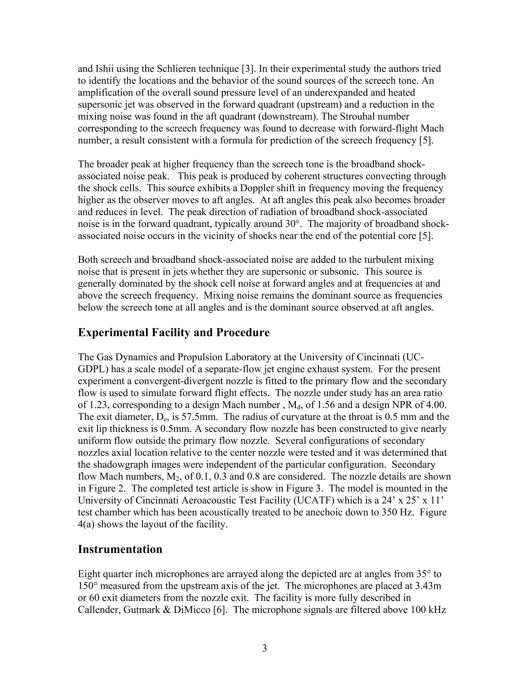
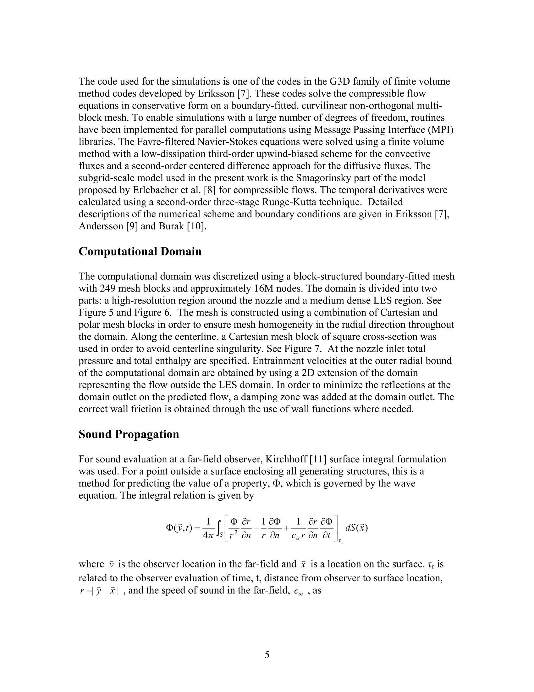
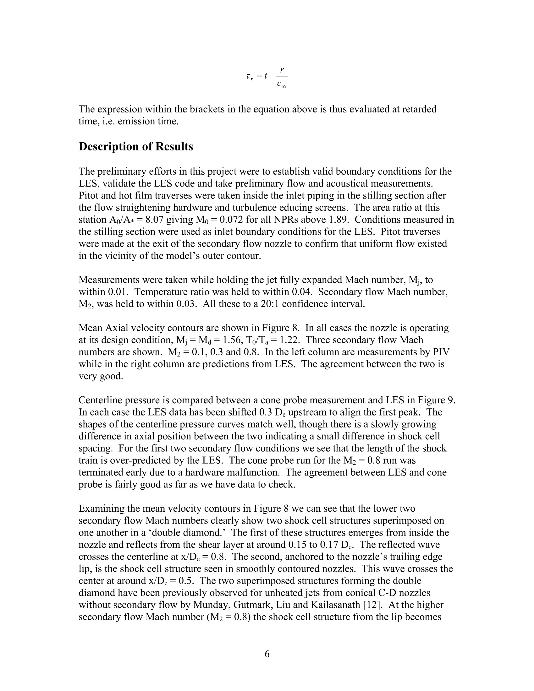
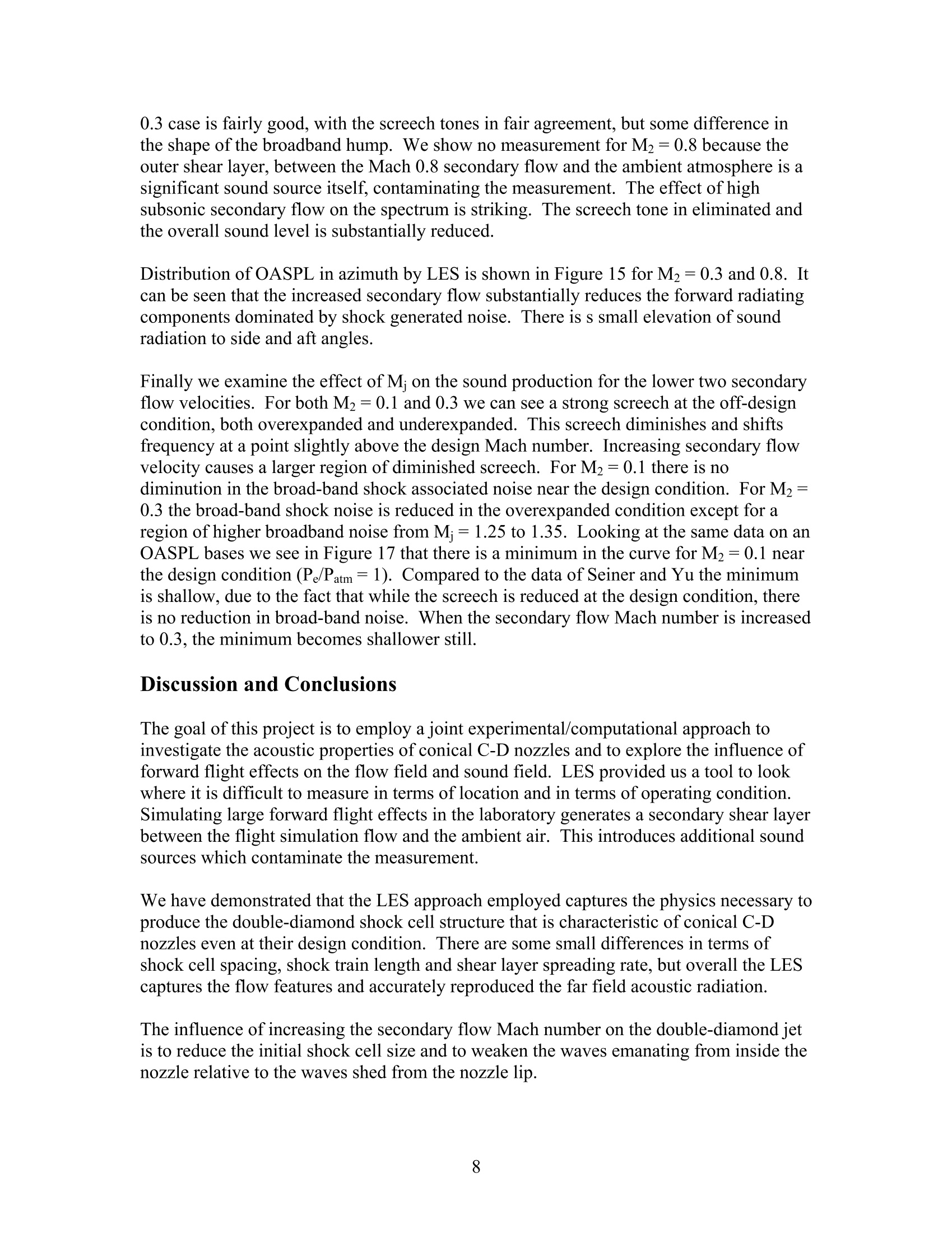
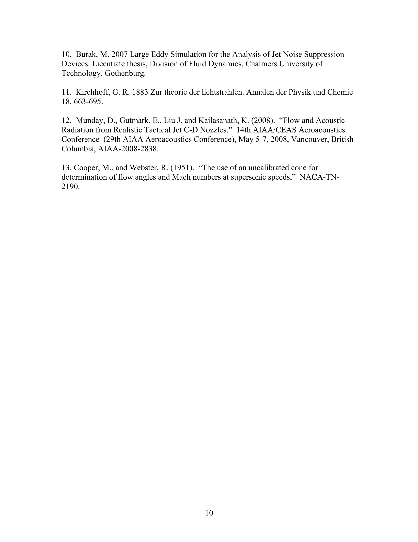
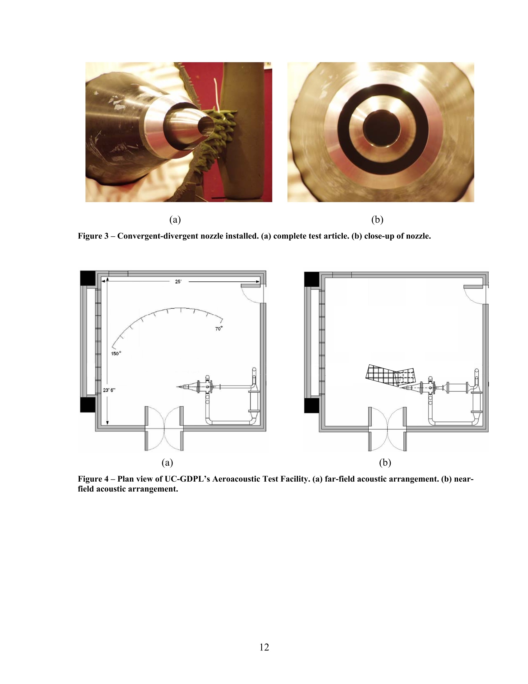
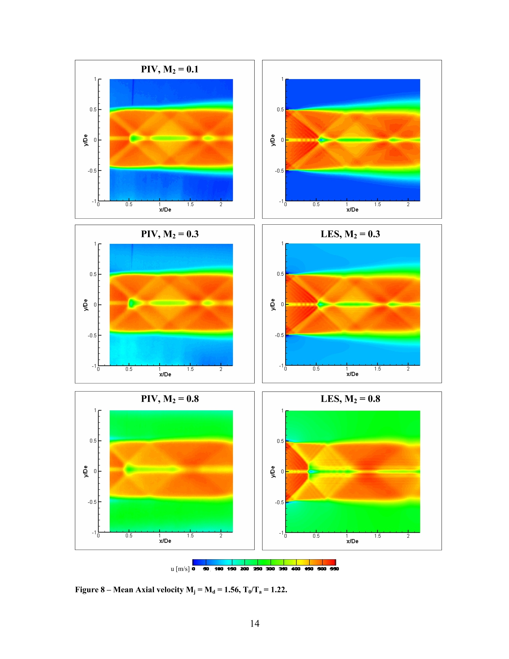
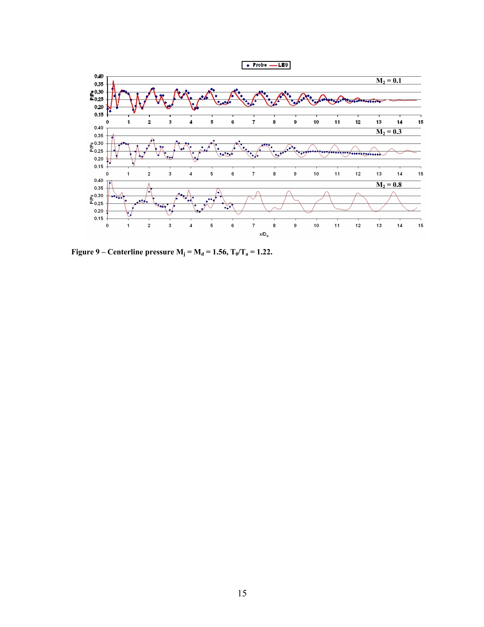
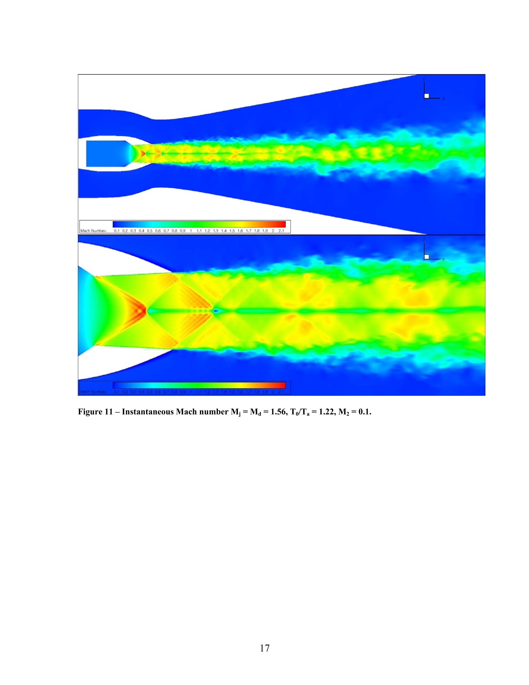
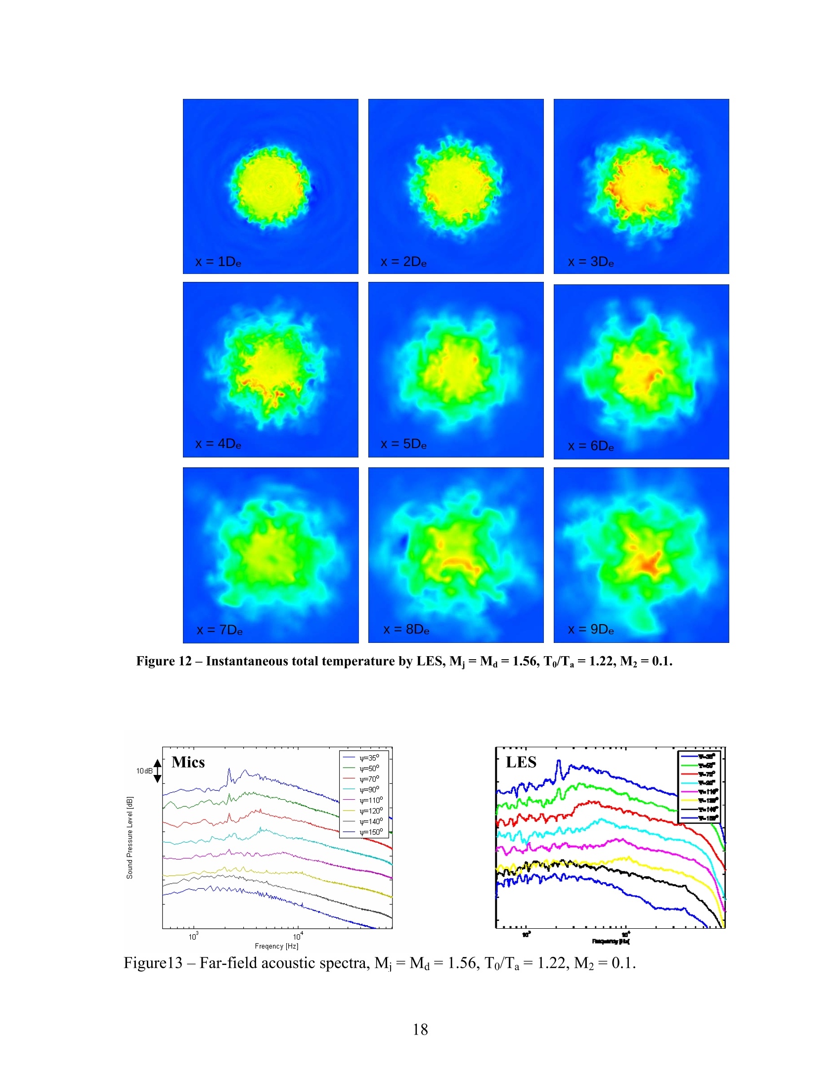
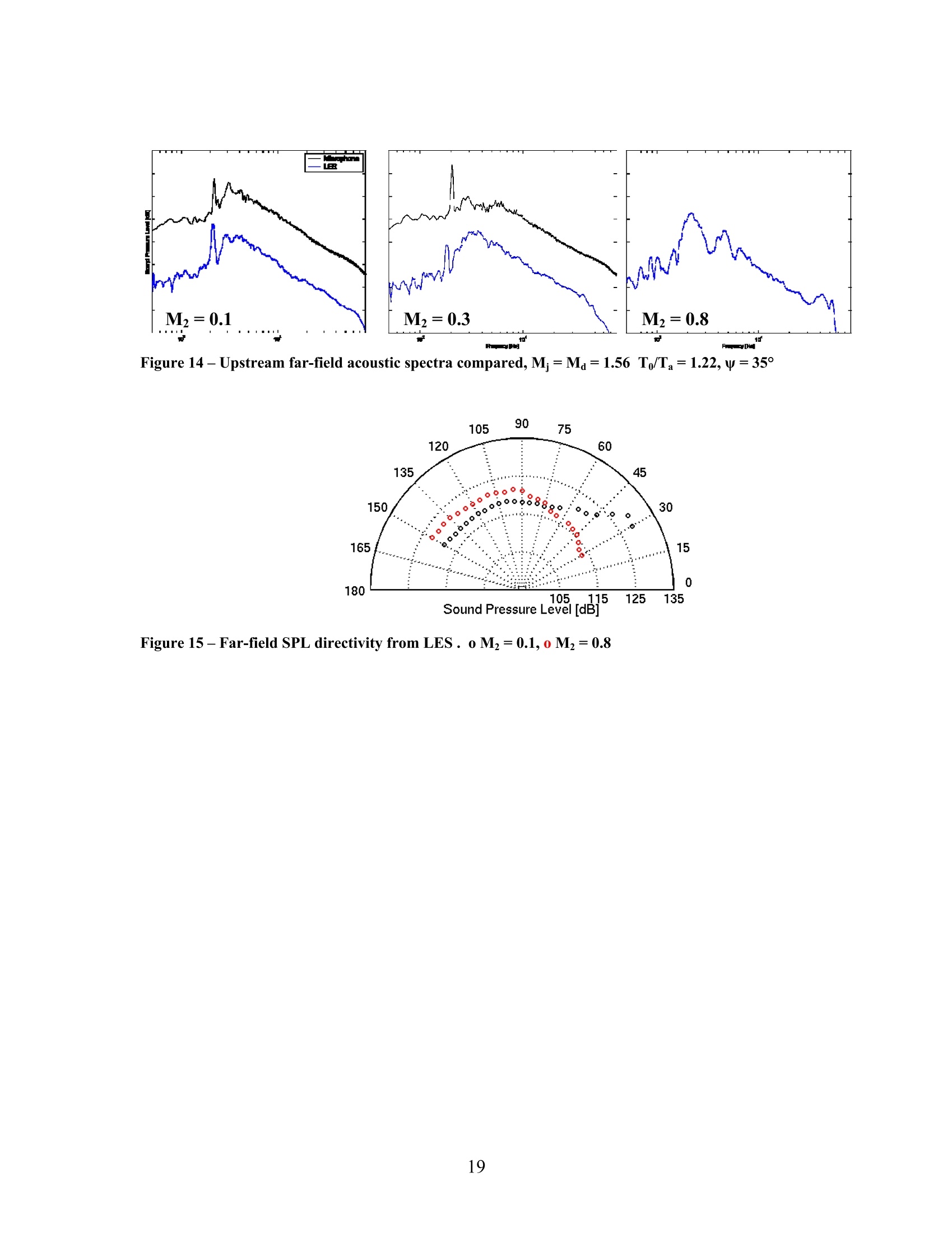
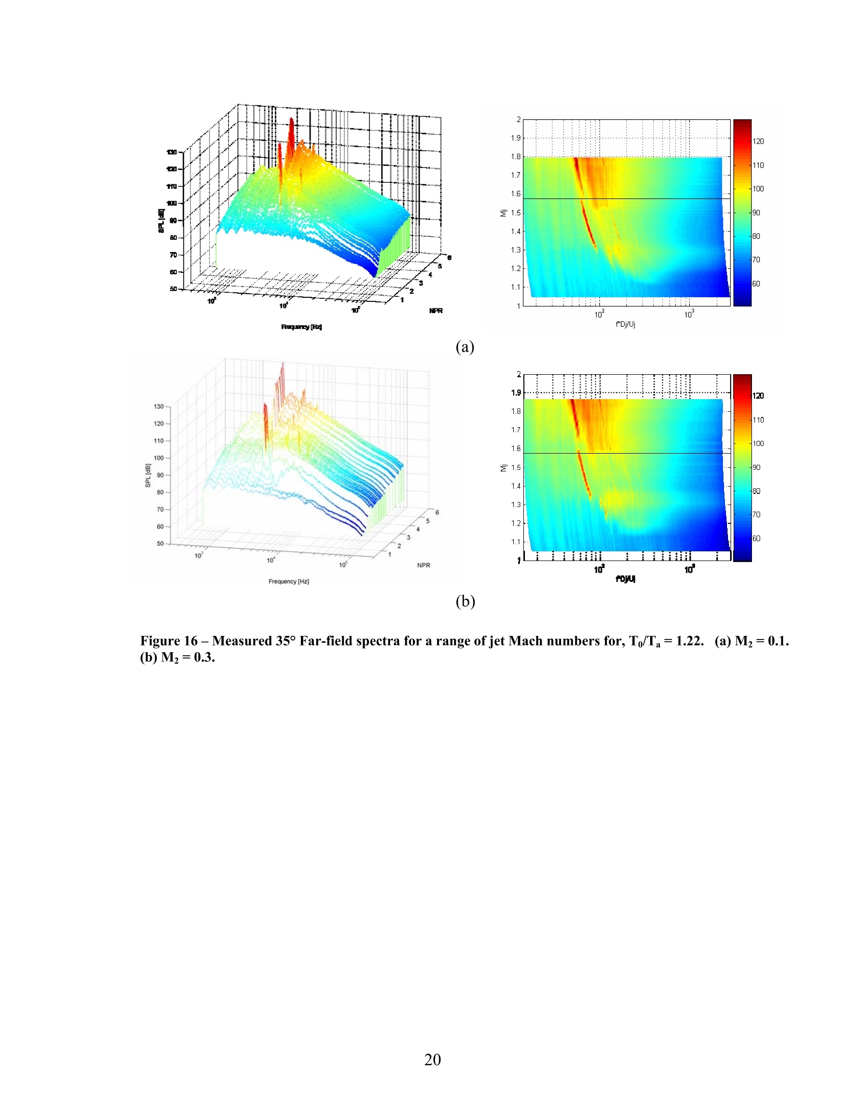
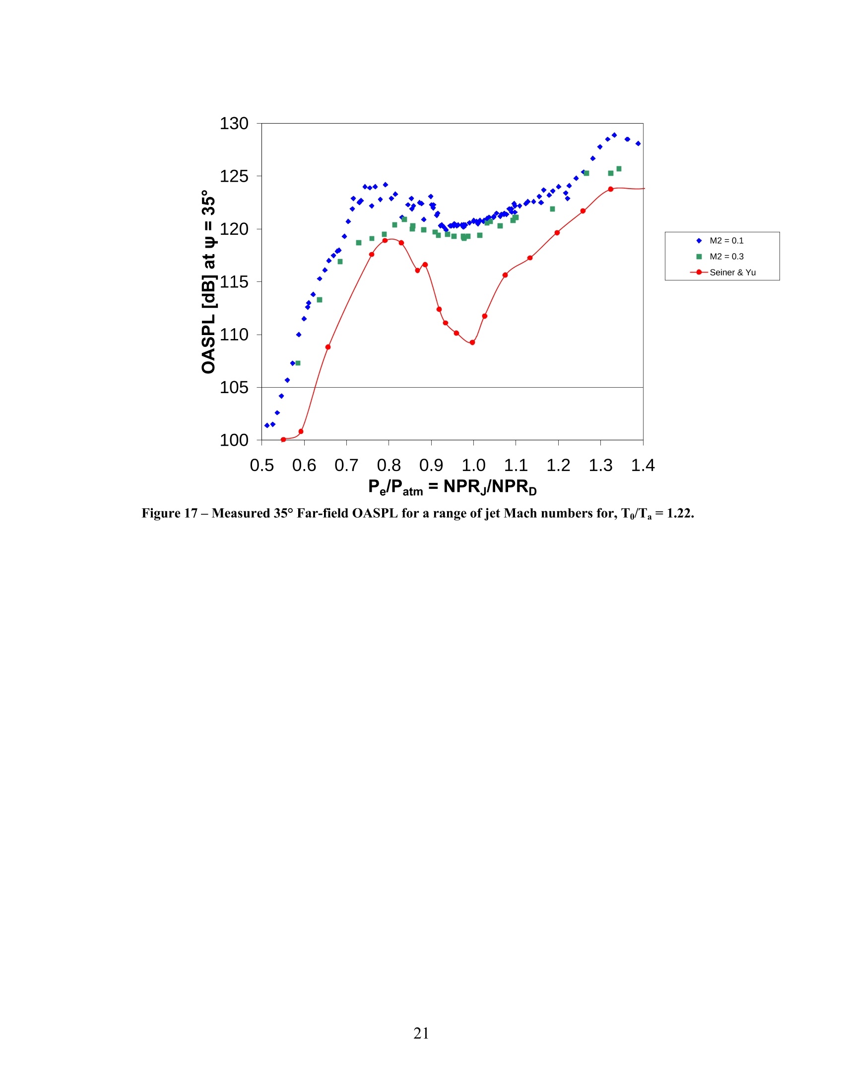
SUPERSONIC JET NOISE FROM A CONICALC-D NOZZLE WITH FORWARD FLIGHTEFFECTS David Munday， Nick Heeb and Ephraim GutmarkUniversity of Cincinnati Markus O. Burak and Lars-Erik Eriksson**Chalmers University ofTechnology Erik PrisellT FMV Flow and far-field noise measurements are taken on a conical Convergent-Divergent nozzle similar to the nozzles employed on high-performancetactical jets. Matching flow and far-field computations are presented，produced by Large Eddy Simulation and the Kirchhoff integral method.The conditions examined are those in which the nozzle is operated at itsdesign Mach number of 1.56 while forward flight is simulated at Machnumbers of 0.1， 0.3 and 0.8. Both measurement and LES show thatincreasing forward flight Mach number to the high subsonic rangeshortens the initial shock cell size， and weakens the shock cells induced bythe nozzle throat relative to the shock cells induced by the nozzle lip. LESshows that high forward flight speed substantially reduces the noiseradiated into the forward quadrant where shock noise is dominant. It alsoremoves the screech tone entirely. Nomenclature a Speed of sound DThroat diameter D Exit diameter LES Large Eddy Simulation MDesign Mach number M Fully expanded jet Mach number NPR Nozzle Pressure Ratio Secondary flow Mach number ( Graduate Student； member AIAA.， david.munday@uc.edu ) ( Graduate Student； member AIAA.，heebns@email.uc.edu ) ( + D istinguished Professor ； Fellow AIAA.， Ephraim.Gutmark@uc.edu ) ( ’Ph.D. Student； member AIAA， mabu@chalmers.se ) ( P rofessor； member AIAA， lee@chalmers.se ) ( Strategic specialist； Aero-propulsion ) Angle from the upstream axis Introduction High-speed military aircraft are typically powered by low-bypass turbofan engines with amixed exhaust， re-heat and a variable geometry convergent-divergent exhaust nozzle. Asthe altitude and operating condition of the engine varies，the nozzles employed adjusts tomatch the mass flow and jet Mach number to some extent， but they have internal flowcontours which are far from ideal and they are rarely shock free. This means that theseengines generally produce shock-associated noise as well as the turbulent mixing noisecharacteristic of subsonic or perfectly expanded jets. The noise levels produced by these jets are quite strong. They produce near-fieldpressures which are hard on personnel， aircraft structure and equipment， and far-fieldnoise which disturbs neighbors around air bases and training areas. Limitation of thisnoise will reduce wear and tear on crews and equipment and reduce noise complaintsfrom those in the neighborhood. There has been a fair amount of work published on noise reduction for subsonic，commercial jet engines. The greatest gains in improving subsonic jets have come byreducing the jet velocity while increasing the jet radius to maintain the desired thrust.Increasing jet radius means increasing engine radius and increasing aircraft drag so thisapproach becomes less desirable as the aircraft velocity increases. Other approaches todecreasing subsonic jet noise usually involve mixing enhancements which reduce thelow-frequency noise while increasing high-frequency noise. When we shift to supersonic jets we have all the problems associated with mixing noiseto contend with， but we also have additional sources of noise resulting from shocks andPrandtl-Meyer waves forming shock cells or shock diamonds in the jet itself. Figure 1 shows a typical far-field spectrum of an imperfectly expanded supersonic jetmeasured upstream of the nozzle exit. The figure depicts the three main noisecomponents as was also described previously [1， 2]. The narrow peak with a Strouhal number of 0.32 is a screech tone. Screech is excited byacoustic waves that are generated by interaction between shear layer vortices and shockstructures in the jet， which propagate upstream and excite flow instabilities at the nozzleslip. These energized structures are convected downstream and further interact with theshocks to form a feedback loop (cite Powell). Screech has been investigated by Umeda and Ishii using the Schlieren technique [3]. In their experimental study the authors triedto identify the locations and the behavior of the sound sources of the screech tone. Anamplification of the overall sound pressure level of an underexpanded and heatedsupersonic jet was observed in the forward quadrant (upstream) and a reduction in themixing noise was found in the aft quadrant (downstream). The Strouhal numbercorresponding to the screech frequency was found to decrease with forward-flight Machnumber， a result consistent with a formula for prediction of the screech frequency[5]. The broader peak at higher frequency than the screech tone is the broadband shock-associated noise peak. This peak is produced by coherent structures convecting throughthe shock cells. This source exhibits a Doppler shift in frequency moving the frequencyhigher as the observer moves to aft angles. At aft angles this peak also becomes broaderand reduces in level. The peak direction of radiation of broadband shock-associatednoise is in the forward quadrant， typically around 30°. The majority of broadband shock-associated noise occurs in the vicinity of shocks near the end of the potential core [5]. Both screech and broadband shock-associated noise are added to the turbulent mixingnoise that is present in jets whether they are supersonic or subsonic. This source isgenerally dominated by the shock cell noise at forward angles and at frequencies at andabove the screech frequency. Mixing noise remains the dominant source as frequenciesbelow the screech tone at all angles and is the dominant source observed at aft angles. Experimental Facility and Procedure The Gas Dynamics and Propulsion Laboratory at the University of Cincinnati (UC-GDPL) has a scale model of a separate-flow jet engine exhaust system. For the presentexperiment a convergent-divergent nozzle is fitted to the primary flow and the secondaryflow is used to simulate forward flight effects. The nozzle under study has an area ratioof 1.23， corresponding to a design Mach number， Md， of 1.56 and a design NPR of 4.00.The exit diameter， De， is 57.5mm. The radius of curvature at the throat is 0.5 mm and theexit lip thickness is 0.5mm. A secondary flow nozzle has been constructed to give nearlyuniform flow outside the primary flow nozzle. Several configurations ofsecondarynozzles axial location relative to the center nozzle were tested and it was determined thatthe shadowgraph images were independent of theparticular configuration. Secondaryflow Mach numbers， M2， of 0.1， 0.3 and 0.8 are considered. The nozzle details are shownin Figure 2. The completed test article is show in Figure 3. The model is mounted in theUniversity of Cincinnati Aeroacoustic Test Facility (UCATF) which is a 24'x 25'x 11’test chamber which has been acoustically treated to be anechoic down to 350 Hz. Figure4(a) shows the layout of the facility. Instrumentation Eight quarter inch microphones are arrayed along the depicted arc at angles from 35° to150° measured from the upstream axis of the jet. The microphones are placed at 3.43mor 60 exit diameters from the nozzle exit. The facility is more fully described inCallender， Gutmark & DiMicco [6]. The microphone signals are filtered above 100 kHz and recorded at 200 kHz for 10 seconds. The flow variables are monitored at 4 Hz inorder to establish and hold the desired operating condition of the model. Variablesrecorded include the ambient conditions in the chamber as well as the flow stagnationtemperature and pressure. In order to map the near-field acoustics， eight microphones are mounted on a linear rakewhich is in turn mounted on a large three-axis traverse. The rake is stepped through arectangular region just outside the main flow region. The resulting grid of pressurefluctuations can then be analyzed on an OASPL basis or the particular spectral rangespertinent to different mechanisms can be mapped to look at source location and directionof propagation. Typical mapped regions are shown in Figure 4(b). Detailed flow-field mapping is performed by Particle Image Velocimetry(PIV). The PIVsystem is built by LaVision and the entire PIV suite， laser and cameras are mounted on atraverse which allows the system to be translated， undisturbed， to any streamwise locationallowing many cross-cuts to be measured without the loss of time in changing setups andwithout the uncertainties which come from repeated adjustment of components. Theflow is seeded with olive oil droplets with diameters on the order of 1 um. A 500 mJNew Wave Research nd：YAG double-pulse laser is passed through sheet-forming opticsto illuminate the seed an the images are captured in stereo by a pair of LaVision 1376 x1040 12-bit PIV cameras. The high gradient features in the flow are visualized by the shadowgraph technique. AnOriel 66056 arc lamp is used for illumination. A pair of 12”parabolic first-surfacemirrors with a 72”focal length are employed to collimate the light before the model andthen to focus the beam after. The image is captured with a LaVision Imager Intensecross-correlation CCD camera with 1376 x 1040 pixel resolution and 12-bit intensityresolution. This gives a spatial resolution on the order of 0.01”or 0.004 throat diameters.A 28-300 zoom lens is mounted to the camera which allows optimization of the field ofview. The aperture is left completely open and exposure is controlled by mounting afilter. Averaging 100 images eliminates the turbulence and gives a clear view of theshock and Prandtl-Meyer waves. Point measurements ofstatic pressure and Mach number are performed using asupersonic five-hole conical probe. The probe， a United Sensor model SDF-15-6-15-600，has a truncated cone with a half angle of 15°， a total pressure port is located at the tip ofthe truncated cone and four side ports are evenly spaced around the conic surface. Whenthe side port pressure values are averaged the Mach number result is insensitive to yawangle changes up to 10°[13]. Numerical approach The evolution of the flow is considered to follow the compressible form of the continuity，momentum and energy equations in which the viscous stress and the heat flux have beendefined using Newton's viscosity law and Fourier’s heat law， respectively. This set ofequations is often referred to as the Navier-Stokes equations. The code used for the simulations is one of the codes in the G3D family of finite volumemethod codes developed by Eriksson [7]. These codes solve the compressible flowequations in conservative form on a boundary-fitted， curvilinear non-orthogonal multi-block mesh. To enable simulations with a large number of degrees of freedom， routineshave been implemented for parallel computations using Message Passing Interface (MPI)libraries. The Favre-filtered Navier-Stokes equations were solved using a finite volumemethod with a low-dissipation third-order upwind-biased scheme for the convectivefluxes and a second-order centered difference approach for the diffusive fluxes. Thesubgrid-scale model used in the present work is the Smagorinsky part of the modelproposed by Erlebacher et al. [8] for compressible flows. The temporal derivatives werecalculated using a second-order three-stage Runge-Kutta technique. Detaileddescriptions of the numerical scheme and boundary conditions are given in Eriksson [7]，Andersson [9] and Burak [10]. Computational Domain The computational domain was discretized using a block-structured boundary-fitted meshwith 249 mesh blocks and approximately 16M nodes. The domain is divided into twoparts： a high-resolution region around the nozzle and a medium dense LES region. SeeFigure 5 and Figure 6. The mesh is constructed using a combination of Cartesian andpolar mesh blocks in order to ensure mesh homogeneity in the radial direction throughoutthe domain. Along the centerline， a Cartesian mesh block of square cross-section wasused in order to avoid centerline singularity. See Figure 7. At the nozzle inlet totalpressure and total enthalpy are specified. Entrainment velocities at the outer radial boundof the computational domain are obtained by using a 2D extension of the domainrepresenting the flow outside the LES domain. In order to minimize the reflections at thedomain outlet on the predicted flow， a damping zone was added at the domain outlet. Thecorrect wall friction is obtained through the use of wall functions where needed. Sound Propagation For sound evaluation at a far-field observer， Kirchhoff [11] surface integral formulationwas used. For a point outside a surface enclosing all generating structures， this is amethod for predicting the value of a property，D， which is governed by the waveequation. The integral relation is given by where y is the observer location in the far-field and元 is a location on the surface. tr isrelated to the observer evaluation of time， t， distance from observer to surface location，r=|y-x|， and the speed of sound in the far-field， c.o ， as The expression within the brackets in the equation above is thus evaluated at retardedtime， i.e. emission time. Description of Results The preliminary efforts in this project were to establish valid boundary conditions for theLES， validate the LES code and take preliminary flow and acoustical measurements.Pitot and hot film traverses were taken inside the inlet piping in the stilling section afterthe flow straightening hardware and turbulence educing screens. The area ratio at thisstation A/A*=8.07 giving Mo=0.072 for all NPRs above 1.89. Conditions measured inthe stilling section were used as inlet boundary conditions for the LES. Pitot traverseswere made at the exit of the secondary flow nozzle to confirm that uniform flow existedin the vicinity of the model’s outer contour. Measurements were taken while holding the jet fully expanded Mach number， Mj， towithin 0.01. Temperature ratio was held to within 0.04. Secondary flow Mach number，M2， was held to within 0.03. All these to a20：1 confidence interval. Mean Axial velocity contours are shown in Figure 8. In all cases the nozzle is operatingat its design condition，Mj=Ma=1.56，To/Ta=1.22. Three secondary flow Machnumbers are shown. Mz=0.1，0.3 and 0.8. In the left column are measurements by PIVwhile in the right column are predictions from LES. The agreement between the two isvery good. Centerline pressure is compared between a cone probe measurement and LES in Figure 9.In each case the LES data has been shifted 0.3 De upstream to align the first peak. Theshapes of the centerline pressure curves match well， though there is a slowly growingdifference in axial position between the two indicating a small difference in shock cellspacing. For the first two secondary flow conditions we see that the length of the shocktrain is over-predicted by the LES. The cone probe run for the M2=0.8 run wasterminated early due to a hardware malfunction. The agreement between LES and coneprobe is fairly good as far as we have data to check. Examining the mean velocity contours in Figure 8 we can see that the lower twosecondary flow Mach numbers clearly show two shock cell structures superimposed onone another in a ‘double diamond.’The first of these structures emerges from inside thenozzle and reflects from the shear layer at around 0.15 to 0.17 De. The reflected wavecrosses the centerline at x/De=0.8. The second， anchored to the nozzle’s trailing edgelip， is the shock cell structure seen in smoothly contoured nozzles. This wave crosses thecenter at aroundx/De=0.5. The two superimposed structures forming the doublediamond have been previously observed for unheated jets from conical C-D nozzleswithout secondary flow by Munday， Gutmark， Liu and Kailasanath [12]. At the highersecondary flow Mach number (M2=0.8) the shock cell structure from the lip becomes slightly shorter， crossing the centerline at x/D。=0.4while the structure from inside thenozzle becomes much less pronounced. At high subsonic secondary flow Mach number the structure from inside the nozzlebecomes indistinct in PIV， but it can still be discerned in shadowgraph. Figure 10 showsshadowgraph images of nine secondary flow Mach numbers ranging from M2 =0.0 to0.8. The vertical lines aid in tracking features in the images. They are aligned with thefeatures in the first image (M2=0.0) and we can see how the features move relative tothis condition in subsequent images. Features associated with the lip wave are marked with green lines. The first green line isat the nozzle lip itself. The second green line， the dashed green line， is aligned with thepoint where lip wave crosses the centerline. This crossing point remains fixed up to M2=0.4 after which it begins to move upstream. The third green line tracks the first reflectionof the lip wave from the shear layer which likewise moves upstream past M2=0.4. Features associated with the wave from inside the nozzle are tracked by the red lines.The first red line follows the first reflection of this wave from the shear layer. Thesecond red line， the dashed one， follows the point at which this reflected internal wavecrosses the centerline. The third red line follows the second reflection of this wave fromthe shear layer. These features also move upstream， but they also become weaker assecondary flow Mach number increases. For M2 above 0.7 is becomes difficult to makeout the center crossing of this wave， but the reflection can be seen as high as M2=0.8. Instantaneous Mach number contours from LES are shown in Figure 11 for M2=0.1.The lower subfigure shows a close-up view of the inside of the nozzle where PIV can notreach. We can see that there is a shock wave shed from the nozzle throat producing aMach disk at x/De=-0.32. The onward traveling shock wave exits the nozzle andreflects from the shear layer at z/De=0.17 or so. The Mach disk sheds a slip line whichis clearly visible in the PIV as well as the LES confirming the details of the in-nozzleflow structure. Looking at instantaneous total temperature in a series of cross-stream planes shows thedevelopment and mixing of the hot high-speed jet with cool lower speed secondary flowin Figure 12. The cross-planes range from x/De=1 to 9. Moving from x/De=1 through3 we can see the jet boundary become convoluted as large scale structures in the shearlayer mix the hot with cold fluid. By x/De=7there is little if any unmixed fluid， butbeyond this point we do see pockets of higher enthalpy as the jet flaps and flickers. Far-field acoustics were measured in the laboratory and calculated from the LES. Spectrafor the nozzle operating at its design condition and Mz=0.1 are shown in Figure13 rangeof inlet angles. In both the measurement and the simulation we see the typical featuresassociated with shock associated noise. A screech tone appears at 2200 Hz with abroadband peak at 2600-5000Hz in the forward-most angle， shifting to higher frequenciesas the observer moves aft. Measurement and simulation are compared in detail for theforward-most angle in Figure 14. The agreement for Mz =0.1 is outstanding. The M= 0.3 case is fairly good， with the screech tones in fair agreement， but some difference inthe shape of the broadband hump. We show no measurement for M2=0.8 because theouter shear layer， between the Mach 0.8 secondary flow and the ambient atmosphere is asignificant sound source itself， contaminating the measurement. The effect of highsubsonic secondary flow on the spectrum is striking. The screech tone in eliminated andthe overall sound level is substantially reduced. Distribution of OASPL in azimuth by LES is shown in Figure 15 for M2=0.3 and 0.8. Itcan be seen that the increased secondary flow substantially reduces the forward radiatingcomponents dominated by shock generated noise. There is s small elevation of soundradiation to side and aft angles. Finally we examine the effect of M on the sound production for the lower two secondaryflow velocities. For both Mz=0.1 and 0.3 we can see a strong screech at the off-designcondition， both overexpanded and underexpanded. This screech diminishes and shiftsfrequency at a point slightly above the design Mach number. Increasing secondary flowvelocity causes a larger region of diminished screech. For M2=0.1 there is nodiminution in the broad-band shock associated noise near the design condition. For M2=0.3 the broad-band shock noise is reduced in the overexpanded condition except for aregion of higher broadband noise from M；=1.25 to 1.35. Looking at the same data on anOASPL bases we see in Figure 17 that there is a minimum in the curve for M2=0.1 nearthe design condition (Pe/Patm=1). Compared to the data of Seiner and Yu the minimumis shallow， due to the fact that while the screech is reduced at the design condition， thereis no reduction in broad-band noise. When the secondary flow Mach number is increasedto 0.3， the minimum becomes shallower still. Discussion and Conclusions The goal of this project is to employ a joint experimental/computational approach toinvestigate the acoustic properties of conical C-D nozzles and to explore the influence offorward flight effects on the flow field and sound field. LES provided us a tool to lookwhere it is difficult to measure in terms of location and in terms of operating condition.Simulating large forward flight effects in the laboratory generates a secondary shear layerbetween the flight simulation flow and the ambient air. This introduces additional soundsources which contaminate the measurement. We have demonstrated that the LES approach employed captures the physics necessary toproduce the double-diamond shock cell structure that is characteristic of conical C-Dnozzles even at their design condition. There are some small differences in terms ofshock cell spacing， shock train length and shear layer spreading rate， but overall the LEScaptures the flow features and accurately reproduced the far field acoustic radiation. The influence of increasing the secondary flow Mach number on the double-diamond jetis to reduce the initial shock cell size and to weaken the waves emanating from inside thenozzle relative to the waves shed from the nozzle lip. LES and CAA enabled us to predict the acoustic radiation at higher secondary flow Machnumber (higher simulated forward flight speed) than we would be able to measure. Wefind that the influence of high subsonic forward flight is to eliminate the screech and tostrongly reduce the forward radiated sound characteristic of shock containing jet noise. Acknowledgements The authors would like to acknowledge the support of the Swedish Defense MaterielAdministration (FMV) which provided financial support for this research and VolvoAero Corporation which provided technical guidance in the design of the nozzle andselection oftest conditions. The computations were performed on computing resourcesat the National Supercomputer Centre in Sweden (NSC). References 1. Seiner， John M. (1984). Advances in High Speed Jet Aeroacoustics. AIAA/NASA 9"Aeroacoustics Conference. AIAA-84-2275. 2. Shih， F. S.， Alvi， D.M. (1999). Effects of Counterflow on the AeroacousticProperties ofa Supersont Jet. Journal of Aircraft， 36：451-457. 3i.. Umeda， Y.， and Ishii，R. (2001).“On the sound sources of screech tones radiatedfrom choked circular jets"J. Acoust. Soc. Am， 110：1845-1858. 4. Tam， C.K.W. (1991).“Jet noise generated by large-scale coherent motion”Aeroacoustics of Flight Vehicles： Theory and Practice， NASA RP 1258， Vol. 1. 5. Seiner，J.M.， Yu， J.C. (1984)."Acoustic near-field properties associated withbroadband shock noise”AIAA Journal， 22：1207-1215. 6. Callender， B.， Gutmark， E. and Dimicco， R. (2002).“The design and validation of acoaxial nozzle acoustic test facility，”AIAA-2002-369. 7. Eriksson， L.-E. 1995 Development and validation of highly modular flow solverversions in g2dflow and g3dflow. Internal report 9970-1162. Volvo Aero Corporation，Sweden. 8.. Erlebacher， G.， Hussaini， M. Y.， Speziale，C. G. & Zang， T. A.1992 Toward thelarge-eddy simulation of compressible turbulent flows. Journal of Fluid Mechanics 238，155-185. 9. Andersson， N. 2005 A study of subsonic turbulent jets and their radiated sound usingLarge-Eddy Simulation. PhD thesis， Division of Fluid Dynamics， Chalmers University ofTechnology，Gothenburg. 10. Burak， M. 2007 Large Eddy Simulation for the Analysis of Jet Noise SuppressionDevices. Licentiate thesis， Division of Fluid Dynamics， Chalmers University ofTechnology， Gothenburg. 11. Kirchhoff， G. R. 1883 Zur theorie der lichtstrahlen. Annalen der Physik und Chemie18， 663-695. 12. Munday， D.， Gutmark， E.， Liu J. and Kailasanath，K. (2008).“Flow and AcousticRadiation from Realistic Tactical Jet C-D Nozzles.”14th AIAA/CEAS AeroacousticsConference (29th AIAA Aeroacoustics Conference)， May 5-7， 2008， Vancouver， BritishColumbia，AIAA-2008-2838. 13. Cooper， M.， and Webster， R. (1951).“The use of an uncalibrated cone fordetermination of flow angles and Mach numbers at supersonic speeds，”NACA-TN-2190. St=fDu Figure 1 -Far-field acoustic spectrum (forward quadrant； w=30°，Mp=1.575，M=1.575，M2=0.1). (a) (b) Figure 2 -Nozzle simulating the exhaust of a tactical jet. (a) entire model showing station definitions； Station0 is the location where inlet measurements are made in the stilling chamber， Station 1 is joint in the wettedsurface between this nozzle and the existing hardware， Station * is the throat， station e is the exit plane of thenozzle (b) nozzle details. De=57.5mm，Area Ratio=1.23， curvature radius at throat=0.5 mm. Exit lipthickness=0.5mm. (a) (b) Figure 3-Convergent-divergent nozzle installed.(a) complete test article. (b) close-up of nozzle. Figure 4- Plan view of UC-GDPL’s Aeroacoustic Test Facility.(a) far-field acoustic arrangement. (b) near-field acoustic arrangement. Figure 5-The computational domain is divided into two sections： a high-resolution region for high resolutionof boundary layers and initial shear layers and a medium-resolution LES region optimized for propagation ofacoustic waves. Figure 6-A slice through the domain at y=0， i.e. a xz-plane in the high-resolution LES region. Figure 7-Slice through the computational domain at constant x， i.e. a yz-plane.Combining Cartesian andpolar grid blocks enhances the radial direction grid homogeneity throughout the domain. u [m/s]0 50140 150200250300340 400501500540 Figure 8-Mean Axial velocity M=Ma=1.56，To/Ta=1.22. Figure 9- Centerline pressure M=Ma=1.56，To/Ta=1.22. Figure 10 -Shadowgraph. One hundred images averaged to suppress turbulence and emphasize shock cells.M=Ma=1.56，To/Ta=1.22. Solid lines descend from reflections at the shear layer in Mz=0.0. Dashed linesdescend from waves crossing the centerline in Mz=0.0. Green lines pertain to the wave from the lip. Redlines pertain to the wave from inside. Figure 11 -Instantaneous Mach number M；=Ma=1.56，To/Ta=1.22，Mz=0.1. Figure 12 -Instantaneous total temperature by LES，M；=Ma=1.56，To/Ta=1.22，Mz=0.1. RiquyH[ Figure13-Far-field acoustic spectra， M；=Ma=1.56，To/Ta=1.22，Mz=0.1. Figure 14 -Upstream far-field acoustic spectra compared，M；=Ma=1.56 To/Ta=1.22，w=35° Figure 15-Far-field SPL directivity from LES . 0 M2=0.1，oMz=0.8 f*Dj/Uj (a) 130- 120- 110- 100- 总90a 80- 70- 60- 50- 10 10 10 NPR Frequency [Hz] roju (b) Figure 16-Measured 35° Far-field spectra for a range of jet Mach numbers for， To/Ta=1.22. (a)Mz=0.1.(b)M2=0.3. 130 ·Seiner & Yu Figure 17 - Measured 35° Far-field OASPL for a range of jet Mach numbers for， T/Ta=1.22.