


方案详情
文
A new method to describe small scale statistical information from passive scalar fields has been
proposed by Wang and Peters (2006). They used direct numerical simulations (DNS) of homogeneous shear
flow to introduce the innovative concept. This novel method determines the local minimum and maximum
points of a fluctuating scalar field via gradient trajectories starting from every grid point in the direction of
the steepest ascending and descending scalar gradients. Relying on gradient trajectories, a dissipation element
is defined as the region of all the grid points the trajectories of which share the same pair of maximum
and minimum points. The procedure has also been successfully applied to various DNS fields of homogeneous
shear turbulence using the three velocity components and the kinetic energy as scalar fields. To validate
statistical properties of these elements derived from DNS (Wang and Peters 2006, 2008), dissipation elements
are for the first time determined based on experimental data of a fully developed turbulent channel
flow. The dissipation elements are deduced from the gradients of the instantaneous fluctuation of the three
velocity components u5, v5, and w5 and the instantaneous kinetic energy k5, respectively. The required 3D velocity
data is obtained investigating a 17.82 × 17.82 × 2.7 mm3 (0.356 × 0.356 × 0.054 ) test volume
using tomographic particle-image velocimetry (Tomo-PIV). The measurements are conducted at a Reynolds
number of 1.7× 10⁴ based on the channel half-height and the bulk velocity U. Detection and analysis of
dissipation elements from the experimental velocity data are presented. The statistical results are compared
to the DNS data from Wang and Peters (2006, 2008).
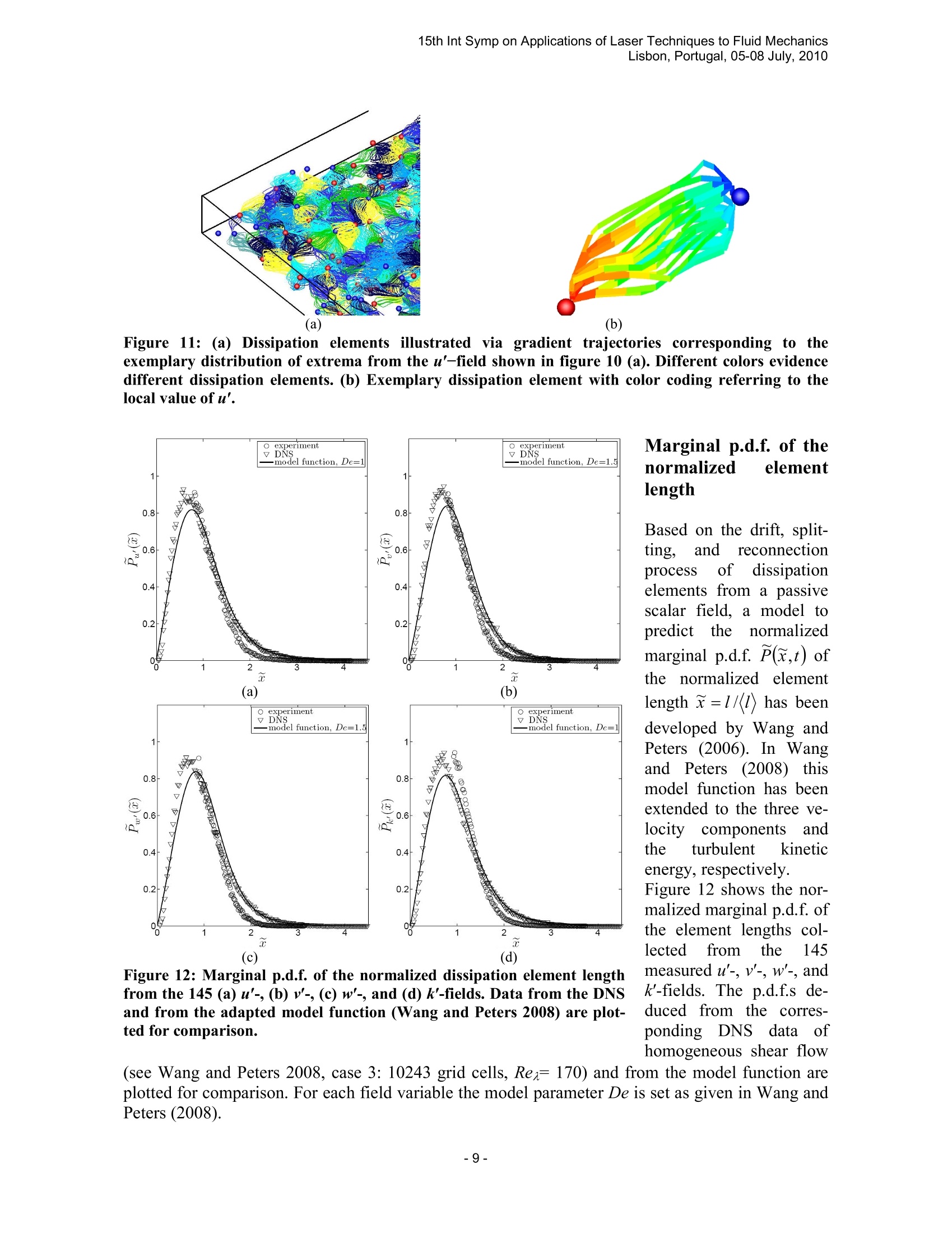
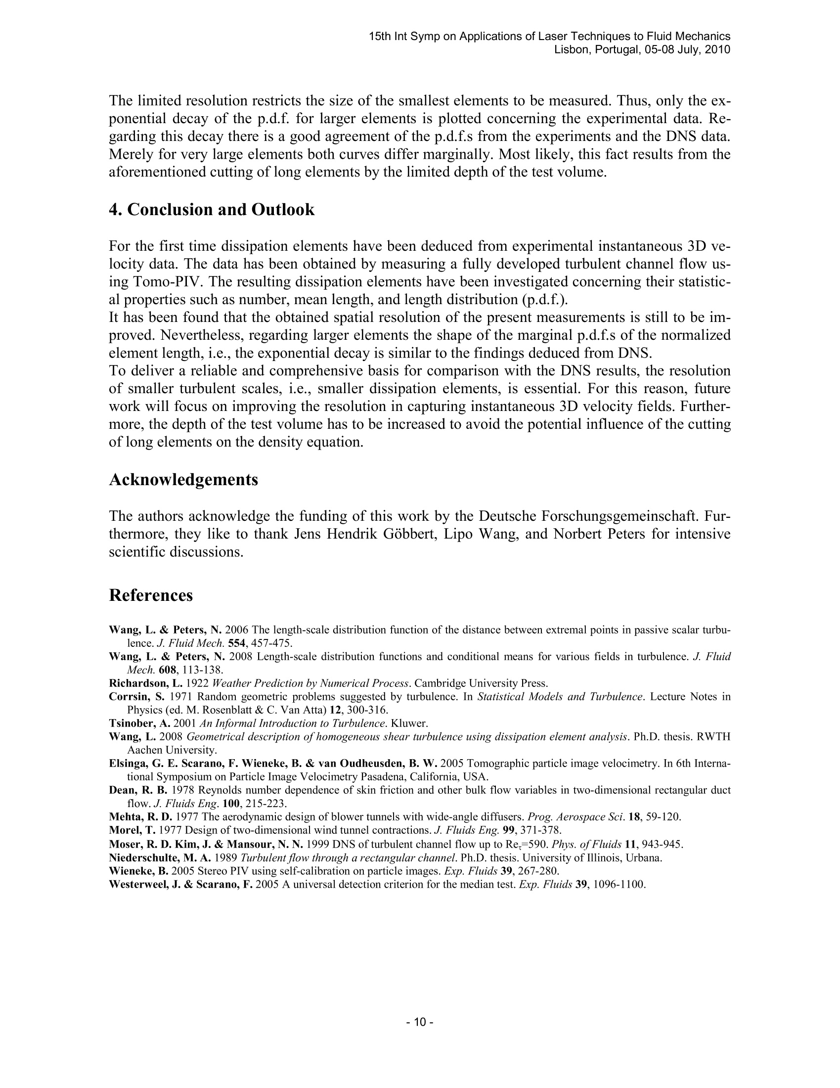
方案详情

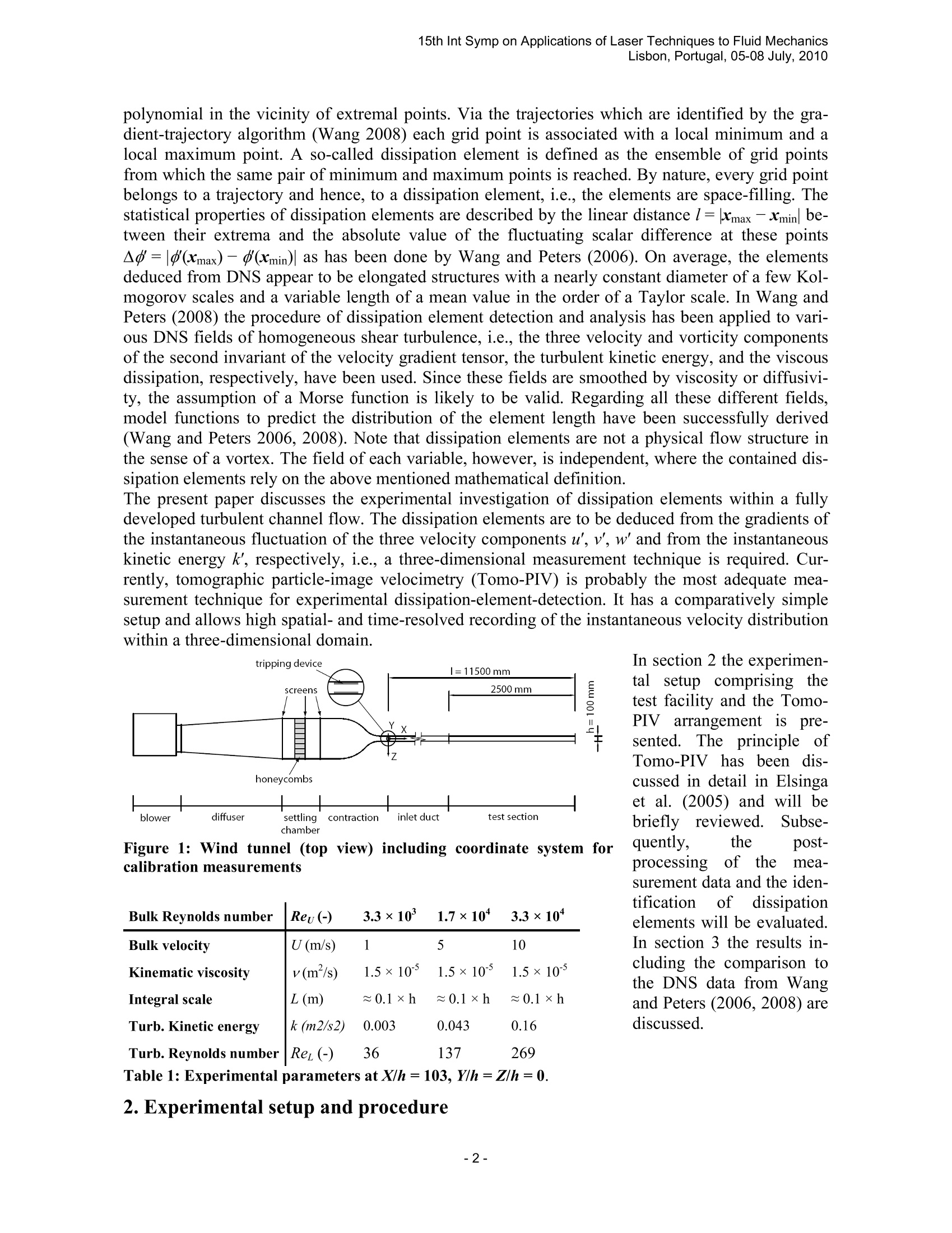
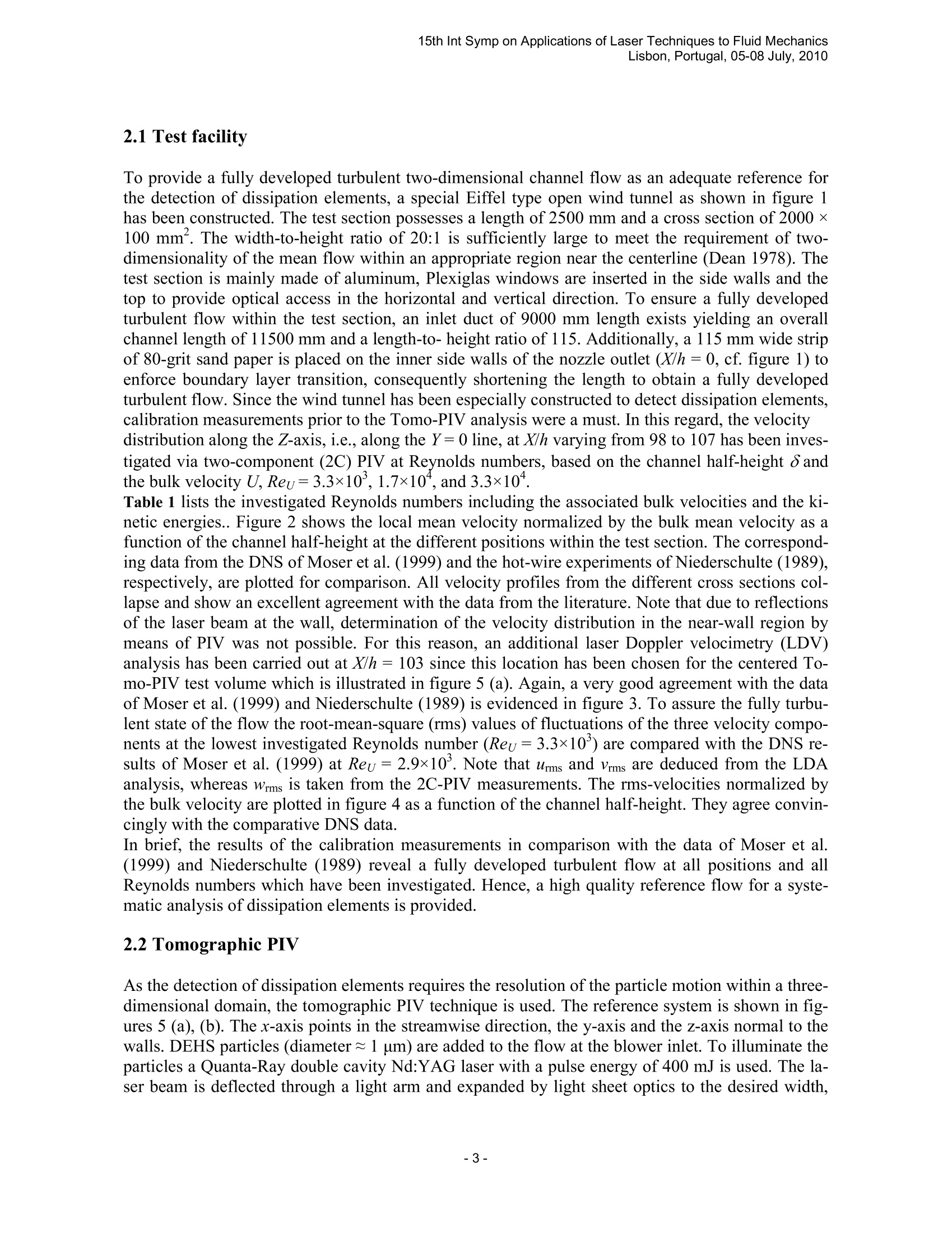
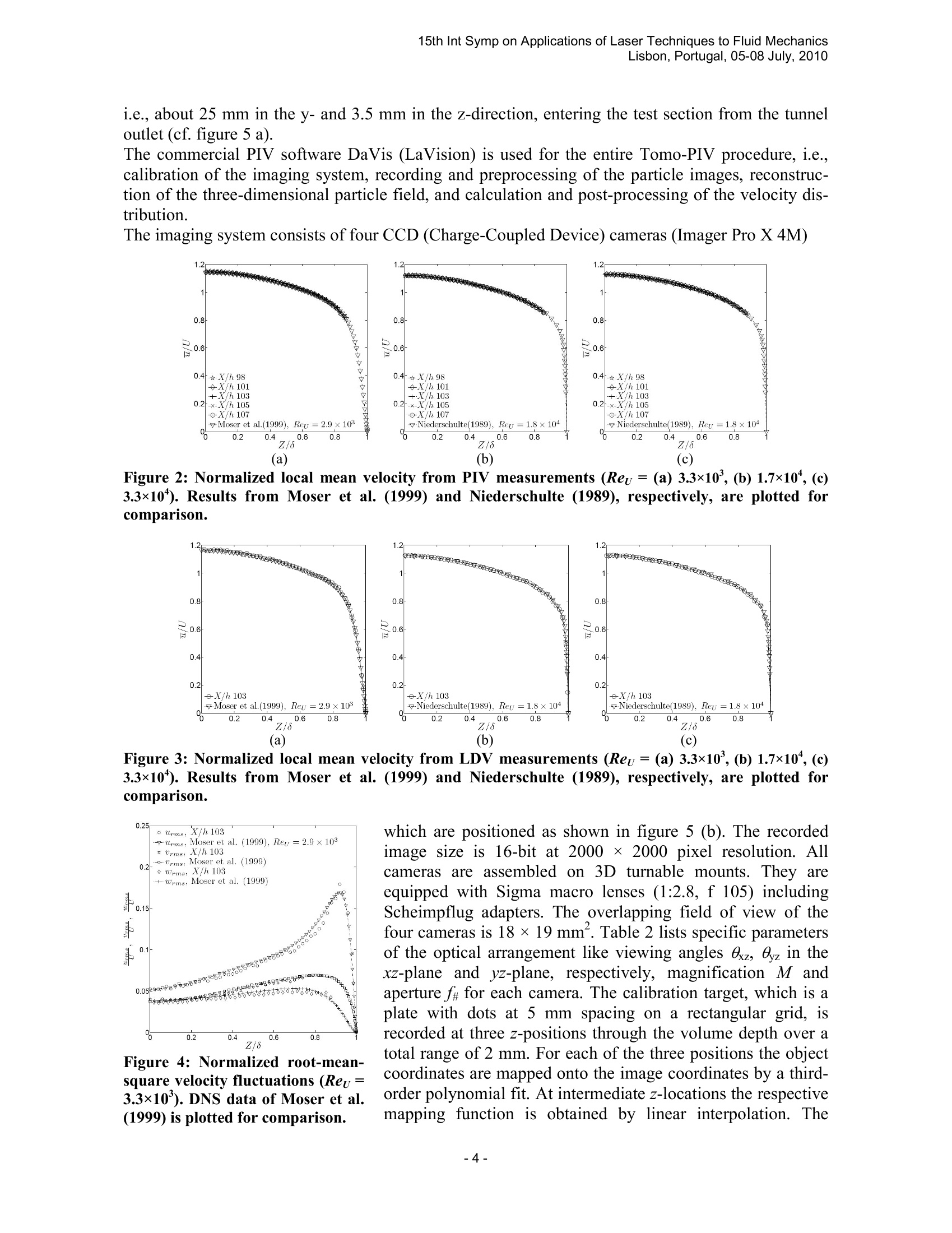
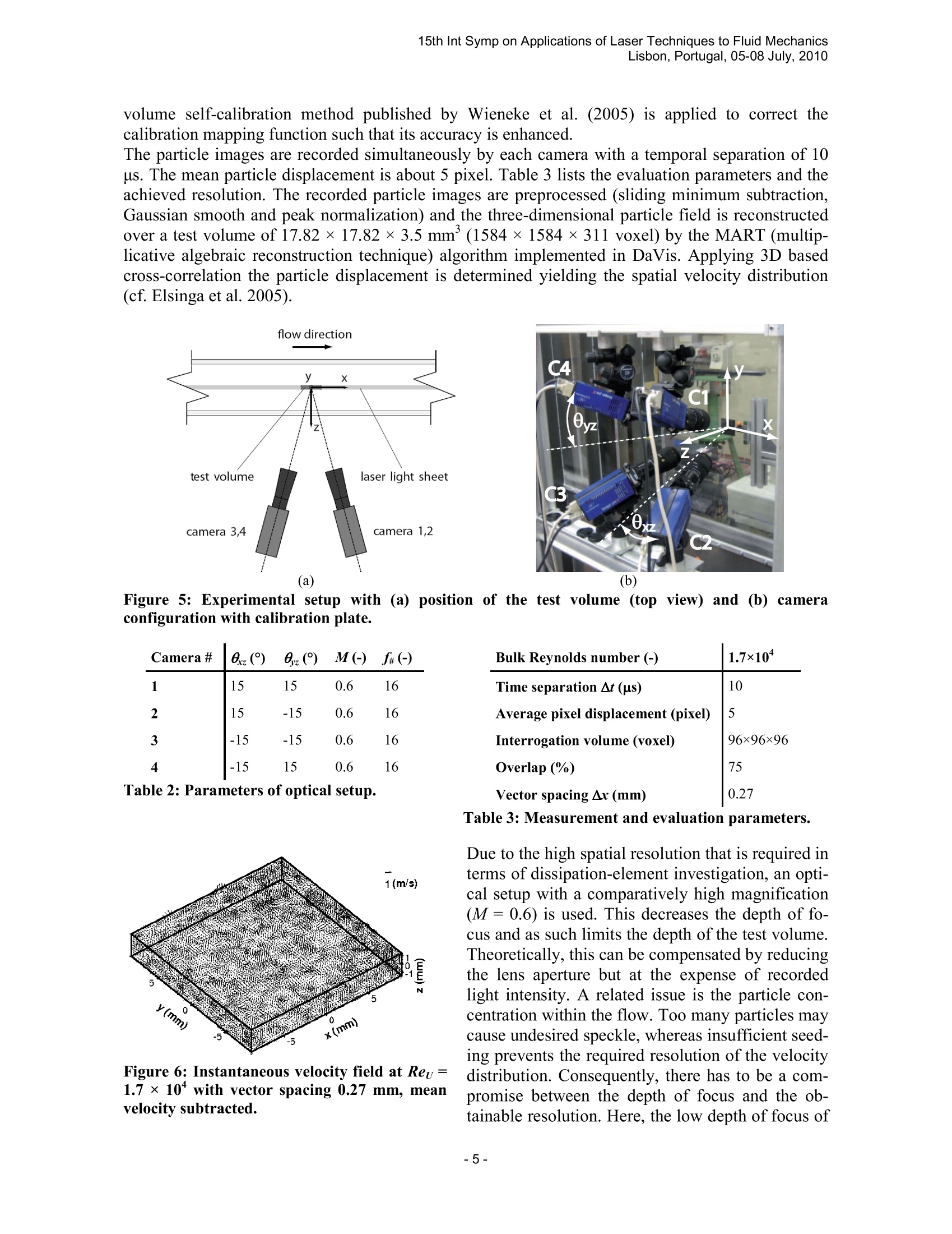
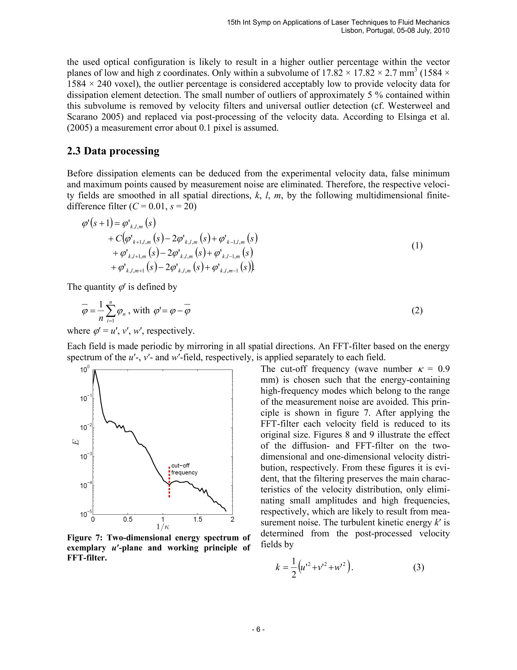
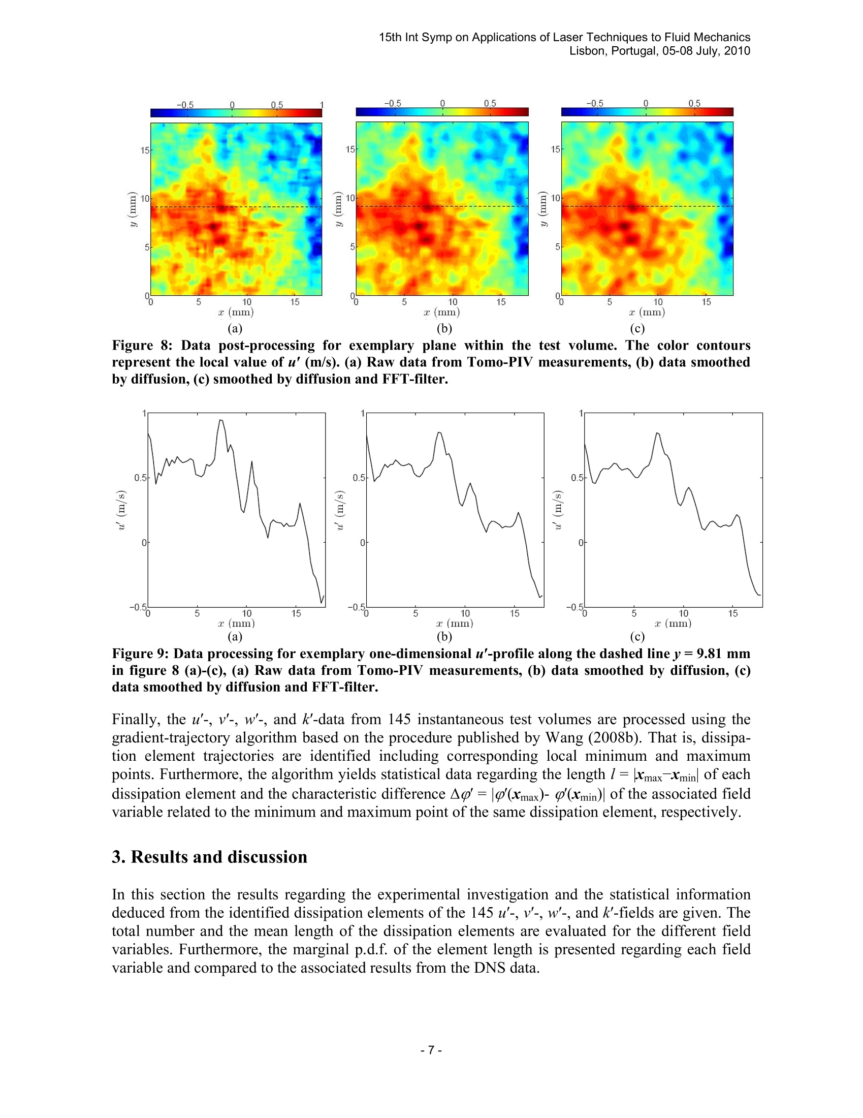
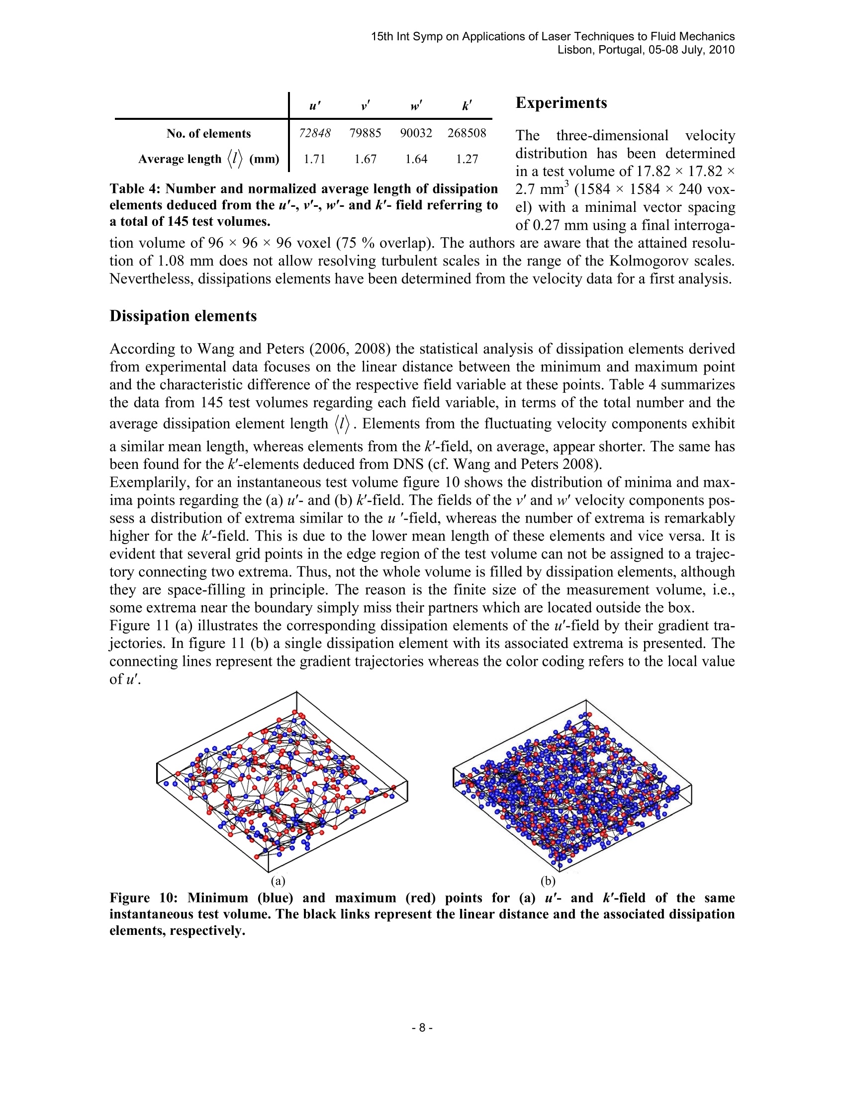
15th Int Symp on Applications of Laser Techniques to Fluid MechanicsLisbon, Portugal, 05-08 July, 2010 Tomographic Particle-Image Velocimetry in a Fully Developed TurbulentChannel Flow to Measure Dissipation Elements Lisa Schafer, Uwe Dierksheide, Michael Klaas , Wolfgang Schroder 1: Institute of Aerodynamics,RWTH Aachen University, Aachen, Germany, l.schaefer@aia.rwth-aachen.de 2: LaVision GmbH, Gottingen, Germany,udierksheide@lavision.de Abstract A new method to describe small scale statistical information from passive scalar fields has beenproposed by Wang and Peters (2006). They used direct numerical simulations (DNS) of homogeneous shearflow to introduce the innovative concept. This novel method determines the local minimum and maximumpoints of a fluctuating scalar field via gradient trajectories starting from every grid point in the direction ofthe steepest ascending and descending scalar gradients. Relying on gradient trajectories, a dissipation ele-ment is defined as the region of all the grid points the trajectories of which share the same pair of maximumand minimum points. The procedure has also been successfully appplpi1ed to various DNS fields of homogene-ous shear turbulence using the three velocity components and the kinetic energy as scalar fields. To validatestatistical properties of these elements derived from DNS (Wang and Peters 2006, 2008), dissipation ele-ments are for the first time determined based on experimental data of a fully developed turbulent channelflow. The dissipation elements are deduced from the gradients of the instantaneous fluctuation of the threevelocity components u',v', and w'and the instantaneous kinetic energy k', respectively. The required 3D ve-locity data is obtained investigating a 17.82×17.82×2.7 mm’(0.356 8×0.356 8×0.054 8) test volumeusing tomographic particle-image velocimetry (Tomo-PIV). The measurements are conducted at a Reynoldsnumber of 1.7x 10 based on the channel half-height 8 and the bulk velocity U. Detection and analysis ofdissipation elements from the experimental velocity data are presented. The statistical results are comparedto the DNS data from Wang and Peters (2006,2008). 1. Introduction Turbulence is a prevalent phenomenon. Despite extensive research, calculation methods to predictthe behavior of turbulent flows still rely on semi-empirical closure-assumptions and models for theintegral scales, i.e., the integral length and time scale. Concerning the small length and time scalesthe comprehension of turbulence is still incomplete. Richardson (1942) introduced the concept of an energy cascade, where turbulence is considered tobe composed of eddies of different sizes. To quantitatively capture the variable length scale withinthe cascade, the entire flow field has to be divided into objects of finite size or spatial regions withsimilar properties, respectively, instead of only dealing with distinct objects as e.g. vortex tubes. Concerning this matter articles of Corrsin (1971) and Tsinober (2001) discussed which kind ofgeometry is naturally identifiable in turbulent flows. Tsinober assumes a certain structure in turbu-lence but remarks that a complex phenomenon as turbulence could probably not be described by anensemble of simple, weakly interacting objects. Hence, it appears convenient to focus on statisticalmethods for the description of geometrical structures in turbulence, where the descriptive parame-ters expediently are geometric lengths. In this spirit, Wang and Peters (2006) proposed a new approach of capturing the nature of turbu-lence. According to this approach, gradient trajectories are identified from fields of a fluctuatingpassive scalar obtained by DNS of homogeneous shear turbulence, starting from each grid point inthe direction of the steepest ascending and descending scalar gradients. These trajectories end atlocal maximum and minimum points, respectively, if the scalar field satisfies the conditions of aMorse function which is a sufficiently smooth function that can be formulated as a second-order polynomial in the vicinity of extremal points. Via the trajectories which are identified by the gra-dient-trajectory algorithm (Wang 2008) each grid point is associated with a local minimum and alocal maximum point. A so-called dissipation element is defined as the ensemble of grid pointsfrom which the same pair of minimum and maximum points is reached. By nature, every grid pointbelongs to a trajectory and hence, to a dissipation element, i.e., the elements are space-filling. Thestatistical properties of dissipation elements are described by the linear distance l=|xmax-Xmin be-tween their extrema and the absolute value of the fluctuating scalar difference at these pointsp=|(xmax)- (xmin)| as has been done by Wang and Peters (2006). On average, the elementsdeduced from DNS appear to be elongated structures with a nearly constant diameter of a few Kol-mogorov scales and a variable length ofa mean value in the order of a Taylor scale. In Wang andPeters (2008) the procedure of dissipation element detection and analysis has been applied to vari-ous DNS fields of homogeneous shear turbulence, i.e., the three velocity and vorticity componentsof the second invariant of the velocity gradient tensor, the turbulent kinetic energy, and the viscousdissipation, respectively, have been used. Since these fields are smoothed by viscosity or diffusivi-ty, the assumption of a Morse function is likely to be valid. Regarding all these different fields,model functions to predict the distribution of the element length have been successfully derived(Wang and Peters 2006, 2008). Note that dissipation elements are not a physical flow structure inthe sense of a vortex. The field of each variable, however, is independent, where the contained dis-sipation elements rely on the above mentioned mathematical definition. The present paper discusses the experimental investigation of dissipation elements within a fullydeveloped turbulent channel flow. The dissipation elements are to be deduced from the gradients ofthe instantaneous fluctuation of the three velocity components u',v, w'and from the instantaneouskinetic energy k', respectively, i.e., a three-dimensional measurement technique is required. Cur-rently, tomographic particle-image velocimetry (Tomo-PIV) is probably the most adequate mea-surement technique for experimental dissipation-element-detection. It has a comparatively simplesetup and allows high spatial-and time-resolved recording of the instantaneous velocity distributionwithin a three-dimensional domain. In section 2 the experimen- Figure 1: Wind tunnel (top view) including coordinate system forcalibration measurements Bulk Reynolds number Reu(-) 3.3×10 1.7×10 3.3×10* Bulk velocity U(m/s) 5 10 Kinematic viscosity v(m’/s) 1.5×10° 1.5×10 1.5×10 Integral scale L(m) ~0.1×h ≈0.1×h ~0.1×h Turb. Kinetic energy k (m2/s2) 0.003 0.043 0.16 Turb.Reynolds number Rez(-) 36 137 269 tal setup comprising thetest facility and the Tomo-PIVarrangement ispre-sented.The principleofTomo-PIV hasbeen dis-cussed in detail in Elsingaet al. (2005) and will bebriefly reviewed.1.Subse-quently, the post-processing of themea-surement data and the iden-tificationnof d(issipationelements will be evaluated.In section 3 the results in-cluding the comparison tothe DNS data from Wangand Peters (2006, 2008) arediscussed. Table 1: Experimental parameters at X/h=103,Y/h=Z/h =0. 2. Experimental setup and procedure 15th Int Symp on Applications of Laser Techniques to Fluid MechanicsLisbon, Portugal, 05-08 July, 2010 2.1 Test facility To provide a fully developed turbulent two-dimensional channel flow as an adequate reference forthe detection of dissipation elements, a special Eiffel type open wind tunnel as shown in figure 1has been constructed. The test section possesses a length of 2500 mm and a cross section of 2000×100 mm. The width-to-height ratio of 20:1 is sufficiently large to meet the requirement of two-dimensionality of the mean flow within an appropriate region near the centerline (Dean 1978). Thetest section is mainly made of aluminum, Plexiglas windows are inserted in the side walls and thetop to provide optical access in the horizontal and vertical direction. To ensure a fully developedturbulent flow within the test section, an inlet duct of 9000 mm length exists yielding an overallchannel length of 11500 mm and a length-to- height ratio of 115. Additionally, a 115 mm wide stripof 80-grit sand paper is placed on the inner side walls of the nozzle outlet (X/h=0, cf. figure 1) toenforce boundary layer transition, consequently shortening the length to obtain a fully developedturbulent flow. Since the wind tunnel has been especially constructed to detect dissipation elements,calibration measurements prior to the Tomo-PIV analysis were a must. In this regard, the velocitydistribution along the Z-axis, i.e., along the Y=0 line, at X/h varying from 98 to 107 has been inves-tigated via two-component (2C) PIV at Reynolds numbers, based on the channel half-height 8 andthe bulk velocity U, Reu=3.3×10’, 1.7×10*, and 3.3x10. Table 1 lists the investigated Reynolds numbers including the associated bulk velocities and the ki-netic energies.. Figure 2 shows the local mean velocity normalized by the bulk mean velocity as afunction of the channel half-height at the different positions within the test section. The correspond-ing data from the DNS ofMoser et al. (1999) and the hot-wire experiments of Niederschulte (1989),respectively,are plotted for comparison. All velocity profiles from the different cross sections col-lapse and show an excellent agreement with the data from the literature. Note that due to reflectionsof the laser beam at the wall, determination of the velocity distribution in the near-wall region bymeans of PIV was not possible. For this reason, an additional laser Doppler velocimetry (LDV)analysis has been carried out at X/h=103 since this location has been chosen for the centered To-mo-PIV test volume which is illustrated in figure 5 (a). Again, a very good agreement with the dataof Moser et al. (1999) and Niederschulte (1989) is evidenced in figure 3. To assure the fully turbu-lent state of the flow the root-mean-square (rms) values of fluctuations of the three velocity compo-nents at the lowest investigated Reynolds number (Reu=3.3×10) are compared with the DNS re-sults of Moser et al. (1999) at Reu=2.9×10. Note that urms and Vrms are deduced from the LDAanalysis, whereas Wrms is taken from the 2C-PIV measurements. The rms-velocities normalized bythe bulk velocity are plotted in figure 4 as a function of the channel half-height. They agree convin-cingly with the comparative DNS data. In brief, the results of the calibration measurements in comparison with the data of Moser et al.(1999) and Niederschulte (1989) reveal a fully developed turbulent flow at all positions and allReynolds numbers which have been investigated. Hence, a high quality reference flow for a syste-matic analysis of dissipation elements is provided. 2.2 Tomographic PIV As the detection of dissipation elements requires the resolution of the particle motion within a three-dimensional domain, the tomographic PIV technique is used. The reference system is shown in fig-ures 5 (a), (b). The x-axis points in the streamwise direction, the y-axis and the z-axis normal to thewalls. DEHS particles (diameter~1 um) are added to the flow at the blower inlet. To illuminate theparticles a Quanta-Ray double cavity Nd:YAG laser with a pulse energy of 400 mJ is used. The la-ser beam is deflected through a light arm and expanded by light sheet optics to the desired width, i.e., about 25 mm in the y- and 3.5 mm in the z-direction, entering the test section from the tunneloutlet (cf. figure 5a). The commercial PIV software DaVis (LaVision) is used for the entire Tomo-PIV procedure, i.e.,calibration of the imaging system, recording and preprocessing of the particle images, reconstruc-tion of the three-dimensional particle field, and calculation and post-processing of the velocity dis-tribution. The imaging system consists of four CCD (Charge-Coupled Device) cameras (Imager Pro X4M) 0.8 .0.6 X/h98 10.8- 0.80.6 .0.6130.44F DD0.4☆X/h98 0.44F☆X/h98O+-X/h 101D +X/h101B+X/h 103B0.2-x-x/h105 0.2-x-X/h 105D-o-X/h 107 -oX/h 107Moser et al.(1999), Reu=2.9×10³ wNiederschulte(1989), Reu=1.8×10⁴ Niederschulte(1989), Reu=1.8×1040.2 0.4 0.6 0.8 0.2 0.4 0.6 0.8 0.2 0.4 0.6 0.8Z/8 Z/8 Z/8(a) (b) (c) +X/h101 +X/h 103 0.2-x-X/h 105 -oX/h107 Figure 2: Normalized local mean velocity from PIV measurements (Reu = (a) 3.3×10, (b) 1.7x10", (c)3.3x10). Results from Moser et al. (1999) and Niederschulte (1989), respectively, are plotted forcomparison. (a) (b) Figure 3: Normalized local mean velocity from LDV measurements (Reu= (a) 3.3x10, (b) 1.7x10", (c)3.3x10). Results from Moser et al. (1999) and Niederschulte (1989), respectively, are plotted forcomparison. Figure 4: Normalized root-mean-square velocity fluctuations (Reu=3.3×10). DNS data of Moser et al.(1999) is plotted for comparison. which are positioned as shown in figure 5 (b). The recordedimage size is 16-bit at 2000 ×2000 pixel resolution. Allcameras are assembled on 3D turnable mounts. They areequipped with Sigma macro lenses (1:2.8, f 105) includingScheimpflug adapters. The overlapping field of view of thefour cameras is 18×19 mm. Table 2 lists specific parametersof the optical arrangement like viewing angles Bxz, Byz in thexz-plane and yz-plane, respectively, magnification M andaperture f# for each camera. The calibration target, which is aplate with dots at 5 mm spacing on a rectangular grid, isrecorded at three z-positions through the volume depth over atotal range of 2 mm. For each of the three positions the objectcoordinates are mapped onto the image coordinates by a third-order polynomial fit. At intermediate z-locations the respectivemapping function is obtained by linear interpolation. The (a) Figure 5: Experimental setup with (a) position of the test volume (top view) and (b) cameraconfiguration with calibration plate. Camera# 0() M(-) )f#(-) 1 15 15 0.6 16 2 15 -15 0.6 16 3 -15 -15 0.6 16 4 -15 15 0.6 16 Table 2: Parameters of optical setup. Table 3: Measurement and evaluation parameters. Due to the high spatial resolution that is required interms of dissipation-element investigation, an opti-cal setup with a comparatively high magnification(M=0.6) is used. This decreases the depth of fo-cus and as such limits the depth of the test volume.Theoretically, this can be compensated by reducingthe lens aperture but at the expense of recordedlight intensity. A related issue is the particle con-centration within the flow. Too many particles maycause undesired speckle, whereas insufficient seed-ing prevents the required resolution of the velocitydistribution. Consequently, there has to be a com-promise between the depth of focus and the ob-tainable resolution. Here, the low depth of focus of the used optical configuration is likely to result in a higher outlier percentage within the vectorplanes of low and high z coordinates. Only within a1 subvolume584 x ?40 YoYf of 17.82×17.82×2.7 mm’(1584×1584 ×240 voxel), the outlier percentage is considered acceptably low to provide velocity data fordissipation element detection. The small number of outliers of approximately 5 % contained withinthis subvolume is removed by velocity filters and universal outlier detection (cf. Westerweel andScarano 2005) and replaced via post-processing of the velocity data. According to Elsinga et al.(2005) a measurement error about 0.1 pixel is assumed. 2.3 Data processing Before dissipation elements can be deduced from the experimental velocity data, false minimumand maximum points caused by measurement noise are eliminated. Therefore, the respective veloci-ty fields are smoothed in all spatial directions, k, l, m, by the following multidimensional finite-difference filter (C=0.01,s=20) The quantity is defined by where '=u',v,w, respectively. Each field is made periodic by mirroring in all spatial directions. An FFT-filter based on the energyspectrum of the u'-,v'- and w’-field, respectively, is applied separately to each field. Figure 7: Two-dimensional energy spectrum ofexemplary u'-plane and working principle ofFFT-filter. The cut-off frequency (wave number K = 0.9mm) is chosen such that the energy-containinghigh-frequency modes which belong to the rangeof the measurement noise are avoided. This prin-ciple is shown in figure 7. After applying theFFT-filter each velocity field is reduced to itsoriginal size. Figures 8 and 9 illustrate the effectof the diffusion- and FFT-filter on the two-dimensional and one-dimensional velocity distri-bution, respectively. From these figures it is evi-dent, that the filtering preserves the main charac-teristics of the velocity distribution, only elimi-nating small amplitudes and high frequencies,respectively, which are likely to result from mea-surement noise. The turbulent kinetic energy k' isdetermined from the post-processed velocityfields by (a) (b) (c) Figure 8: Data post-processing for exemplary plane within the test volume. The color contoursrepresent the local value of u'(m/s). (a) Raw data from Tomo-PIV measurements, (b) data smoothedby diffusion, (C) smoothed by diffusion and FFT-filter. 0.5 0 -0.5 Figure 9: Data processing for exemplary one-dimensional u'-profile along the dashed line y=9.81 mmin figure 8(a)-(C), (a) Raw data from Tomo-PIV measurements, (b) data smoothed by diffusion, (C)data smoothed by diffusion and FFT-filter. Finally, the u'-, v'-,w’-, and k'-data from 145 instantaneous test volumes are processed using thegradient-trajectory algorithm based on the procedure published by Wang (2008b). That is, dissipa-tion element trajectories are identified including corresponding local minimum and maximumpoints. Furthermore, the algorithm yields statistical data regarding the length l=xmaxXmin of eachdissipation element and the characteristic difference Ap'='(xmax)-(Xmin)| of the associated fieldvariable related to the minimum and maximum point of the same dissipation element, respectively. 3. Results and discussion In this section the results regarding the experimental investigation and the statistical informationdeduced from the identified dissipation elements of the 145 u'-,V'-,w'-, and k'-fields are given. Thetotal number and the mean length ofthe dissipation elements are evaluated for the different fieldvariables. Furthermore, the marginal p.d.f. of the element length is presented regarding each fieldvariable and compared to the associated results from the DNS data. u' k’ Experiments No. of elements Average length (I) (mm) Table 4: Number and normalized average length of dissipationelements deduced from the u'-,v'-, w'-and k’-field referring toa total of 145 test volumes. Theetthree-dimensional velocitydistribution has been determinedin a test volume of 17.82×17.82×2.7 mm (1584×1584×240 vox-el) with a minimal vector spacingof 0.27 mm using a final interroga- tion volume of 96×96×96 voxel (75% overlap). The authors are aware that the attained resolu-tion of 1.08 mm does not allow resolving turbulent scales in the range of the Kolmogorov scales.Nevertheless, dissipations elements have been determined from the velocity data for a first analysis. Dissipation elements According to Wang and Peters (2006, 2008) the statistical analysis of dissipation elements derivedfrom experimental data focuses on the linear distance between the minimum and maximum pointand the characteristic difference of the respective field variable at these points. Table 4 summarizesthe data from 145 test volumes regarding each field variable, in terms ofthe total number and theaverage dissipation element length (I). Elements from the fluctuating velocity components exhibita similar mean length,whereas elements from the k'-field, on average, appear shorter. The same hasbeen found for the k'-elements deduced from DNS (cf. Wang and Peters 2008). Exemplarily, for an instantaneous test volume figure 10 shows the distribution of minima and max-ima points regarding the (a) u'-and (b) k’-field. The fields of the v'and w'velocity components pos-sess a distribution of extrema similar to the u '-field, whereas the number of extrema is remarkablyhigher for the k'-field. This is due to the lower mean length of these elements and vice versa. It isevident that several grid points in the edge region of the test volume can not be assigned to a trajec-tory connecting two extrema. Thus, not the whole volume is filled by dissipation elements, althoughthey are space-filling in principle. The reason is the finite size of the measurement volume, i.e.,some extrema near the boundary simply miss their partners which are located outside the box. Figure 11 (a) illustrates the corresponding dissipation elements of the u'-field by their gradient tra-jectories. In figure 11 (b) a single dissipation element with its associated extrema is presented. Theconnecting lines represent the gradient trajectories whereas the color coding refers to the local valueofu'. Figure 10: Minimum (blue) and maximum (red) points for (a) u'- and k'-field of the sameinstantaneous test volume. The black links represent the linear distance and the associated dissipationelements, respectively. (a) (b) Figure 11::((a)Dissipation elements illustrated viaagradient trajectories corresponding to theexemplary distribution of extrema from the u'-field shown in figure 10 (a). Different colors evidencedifferent dissipation elements. (b) Exemplary dissipation element with color coding referring to thelocal value of u'. Marginal p.d.f. of thenormalized elementlength Based on the drift, split-ting, andl reconnectionprocessof ddissipationelements from a passivescalar field, a model topredictthe normalizedmarginal p.d.f. P(x,t) ofthe normalized elementlength x=I/(1) has beendeveloped by Wang andPeters (2006). In Wangand Peters (2008) thismodel function has beenextended to the three ve-locity componentsandthe turbulent kineticenergy,respectively. Figure 12: Marginal p.d.f. of the normalized dissipation element lengthfrom the 145 (a) u'-, (b)v'-,(c) w'-, and (d) k'-fields. Data from the DNSand from the adapted model function (Wang and Peters 2008) are plot-ted for comparison. Figure 12 shows the nor-malized marginal p.d.f. ofthe element lengths col-lected from the 145measured u'-, v'-, w'-, andk'-fields. The p.d.f.s de-duced from the corres-pondingDNSdataofhomogeneous shear flow (see Wang and Peters 2008, case 3: 10243 grid cells, Rex=170) and from the model function areplotted for comparison. For each field variable the model parameter De is set as given in Wang andPeters (2008). The limited resolution restricts the size of the smallest elements to be measured. Thus, only the ex-ponential decay of the p.d.f. for larger elements is plotted concerning the experimental data. Re-garding this decay there is a good agreement of the p.d.f.s from the experiments and the DNS data.Merely for very large elements both curves differ marginally. Most likely, this fact results from theaforementioned cutting of long elements by the limited depth of the test volume. 4. Conclusion and Outlook For the first time dissipation elements have been deduced from experimental instantaneous 3D ve-locity data. The data has been obtained by measuring a fully developed turbulent channel flow us-ing Tomo-PIV. The resulting dissipation elements have been investigated concerning their statistic-al properties such as number, mean length, and length distribution (p.d.f.). It has been found that the obtained spatial resolution of the present measurements is still to be im-proved. Nevertheless, regarding larger elements the shape of the marginal p.d.f.s of the normalizedelement length, i.e., the exponential decay is similar to the findings deduced from DNS. To deliver a reliable and comprehensive basis for comparison with the DNS results, the resolutionof smaller turbulent scales, i.e., smaller dissipation elements, is essential. For this reason, futurework will focus on improving the resolution in capturing instantaneous 3D velocity fields. Further-more, the depth of the test volume has to be increased to avoid the potential influence of the cuttingof long elements on the density equation. Acknowledgements The authors acknowledge the funding of this work by the Deutsche Forschungsgemeinschaft. Fur-thermore, they like to thank Jens Hendrik Gobbert, Lipo Wang, and Norbert Peters for intensivescientific discussions. References Wang, L.& Peters, N. 2006 The length-scale distribution function of the distance between extremal points in passive scalar turbu-lence.J. Fluid Mech. 554, 457-475. Wang, L. & Peters, N. 2008 Length-scale distribution functions and conditional means for various fields in turbulence. J. FluidMech. 608,113-138. Richardson, L. 1922 Weather Prediction by Numerical Process. Cambridge University Press. Corrsin, S. 1971 Random geometric problems suggested by turbulence. In Statistical Models and Turbulence.Lecture Notes inPhysics (ed. M. Rosenblatt & C. Van Atta) 12, 300-316. Tsinober, A. 2001 An Informal Introduction to Turbulence. Kluwer. Wang, L. 2008 Geometrical description of homogeneous shear turbulence using dissipation element analysis. Ph.D. thesis. RWTHAachen University. Elsinga, G. E. Scarano, F. Wieneke, B. & van Oudheusden, B. W. 2005 Tomographic particle image velocimetry. In 6th Interna-tional Symposium on Particle Image Velocimetry Pasadena, California, USA. ( Dean, R. B. 1978 R e ynolds number dep e ndence of s k in friction and other bulk flo w variables in two-dimensional rectangular duct flow.J. Fluids Eng. 1 00, 215-223. ) ( Mehta, R . D. 1977 The aerodynamic design of blower tunnels with wide - angle diffusers. Prog . Aerospace Sci. 18, 59-120. Morel, T. 1 977 Design of two-dimensional wind tunnel contractions. J. Fluids Eng. 99,371-378. ) Moser, R. D. Kim, J. & Mansour, N. N.1999 DNS of turbulent channel flow up to Re=590. Phys. ofFluids 11, 943-945.Niederschulte, M. A. 1989 Turbulent flow through a rectangular channel. Ph.D. thesis. University of Illinois, Urbana.Wieneke, B. 2005 Stereo PIV using self-calibration on particle images. Exp. Fluids 39, 267-280. Westerweel, J. & Scarano, F. 2005 A universal detection criterion for the median test. Exp. Fluids 39, 1096-1100. -- --
确定
还剩8页未读,是否继续阅读?

产品配置单

北京欧兰科技发展有限公司为您提供《湍动槽中采用层析粒子成像测速技术来测量耗散元素检测方案(粒子图像测速)》,该方案主要用于其他中采用层析粒子成像测速技术来测量耗散元素检测,参考标准--,《湍动槽中采用层析粒子成像测速技术来测量耗散元素检测方案(粒子图像测速)》用到的仪器有德国LaVision PIV/PLIF粒子成像测速场仪
推荐专场


相关方案
更多
该厂商其他方案
更多