湍动边界层,近壁面湍流,流体中流场,速度矢量场,速度场检测方案(粒子图像测速)

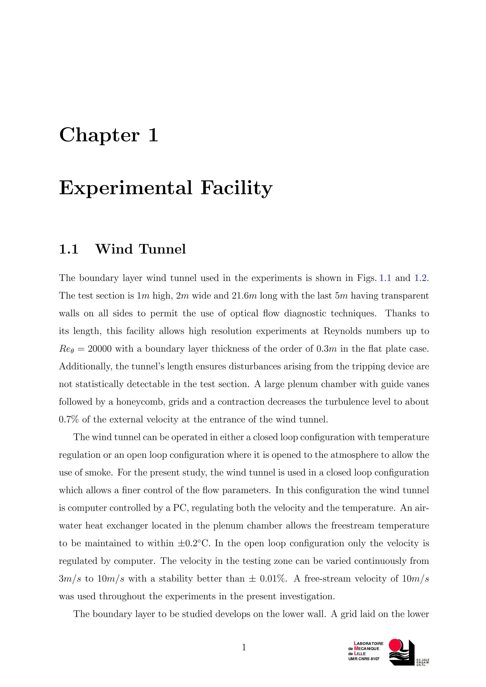
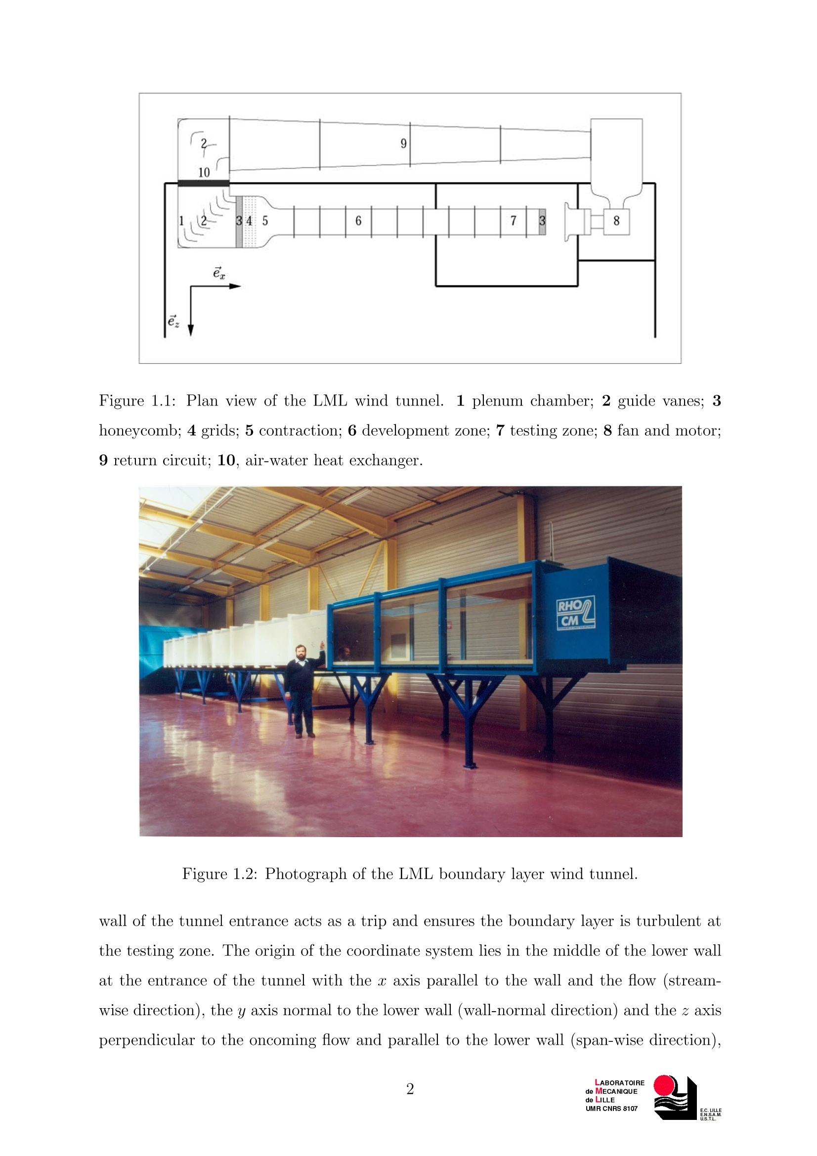
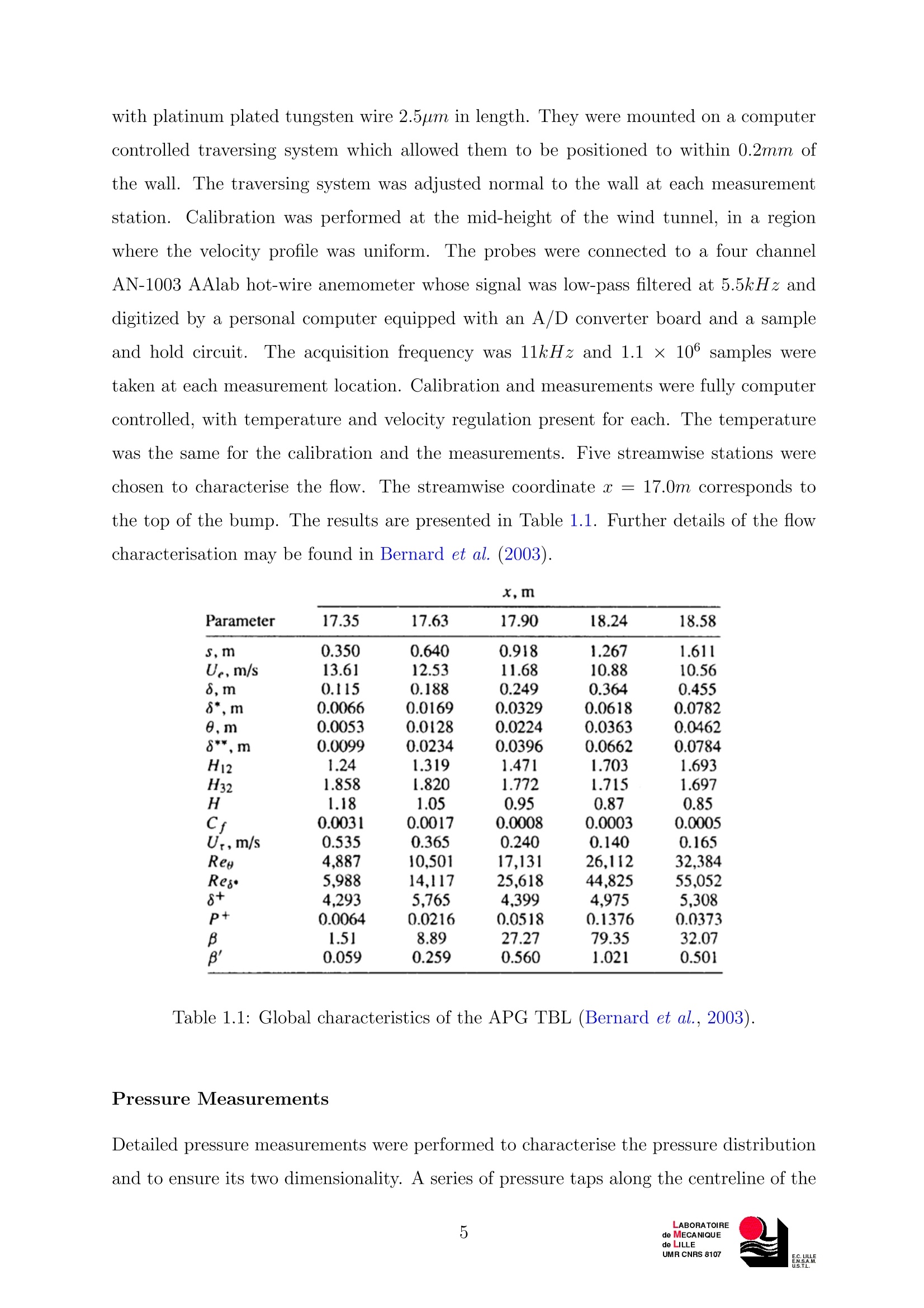
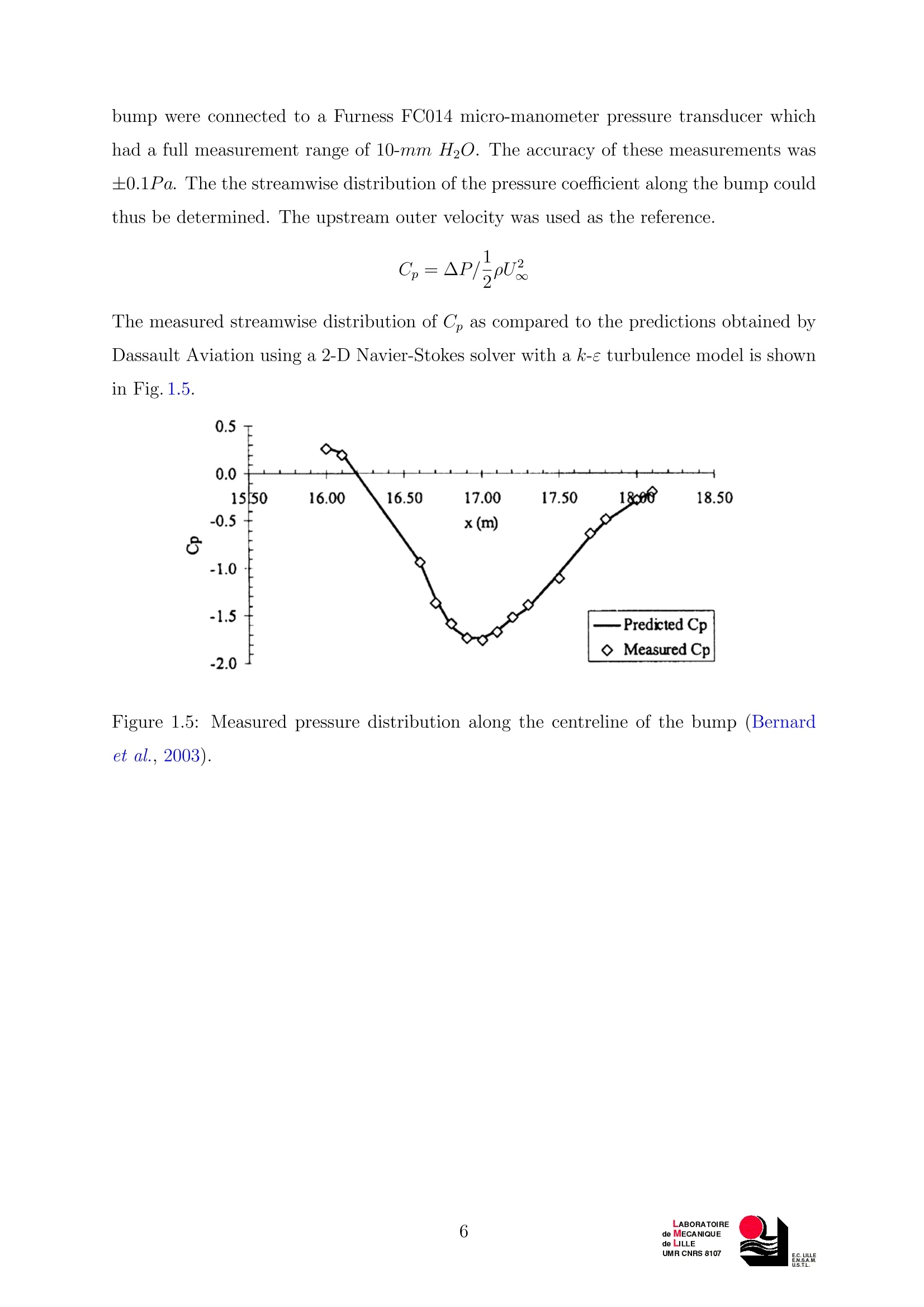
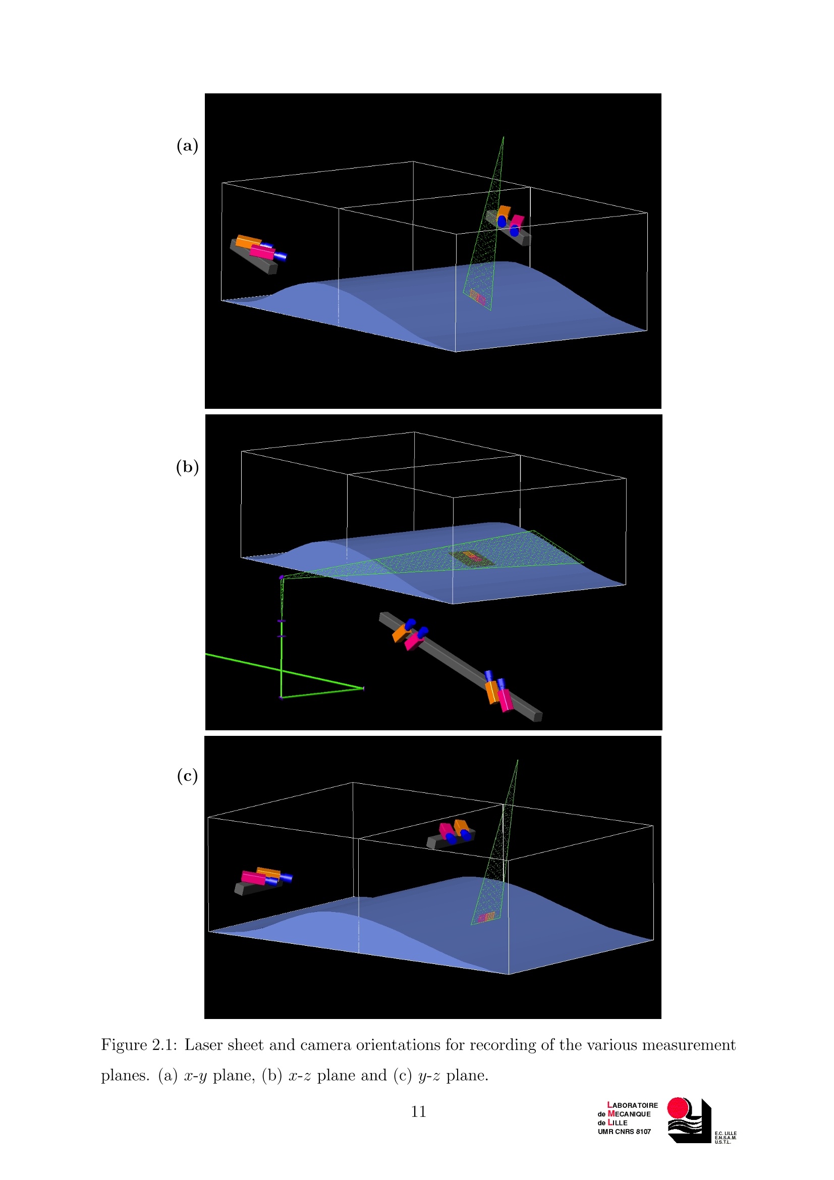
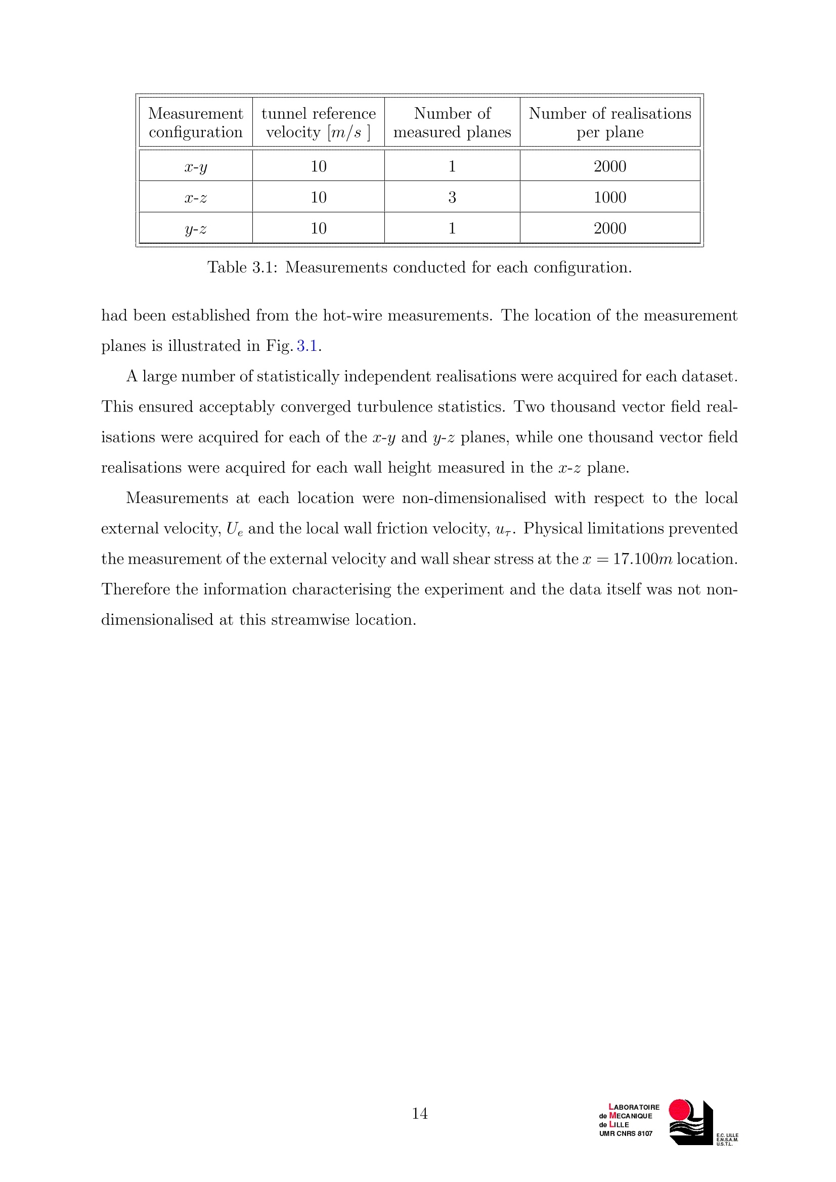
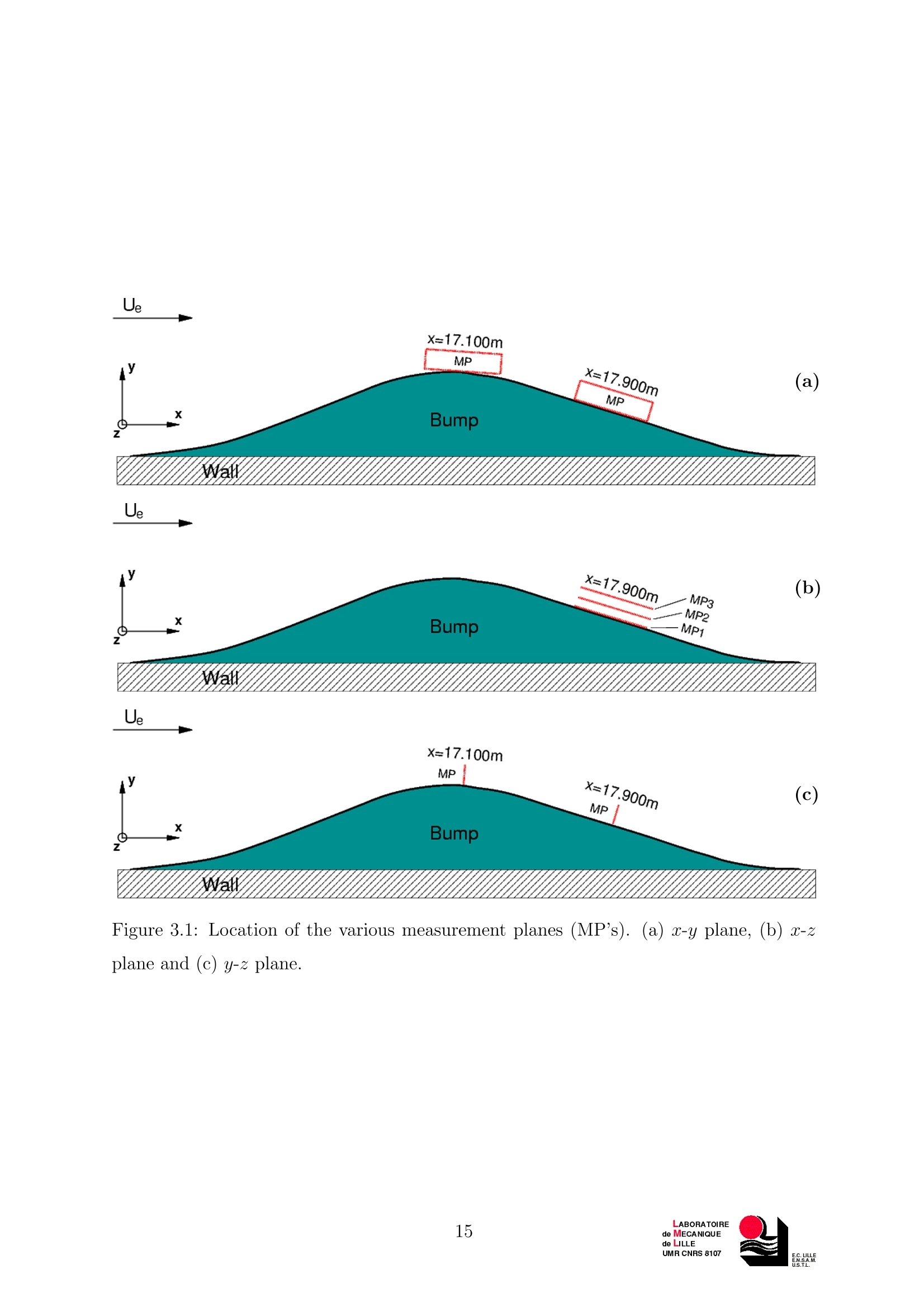
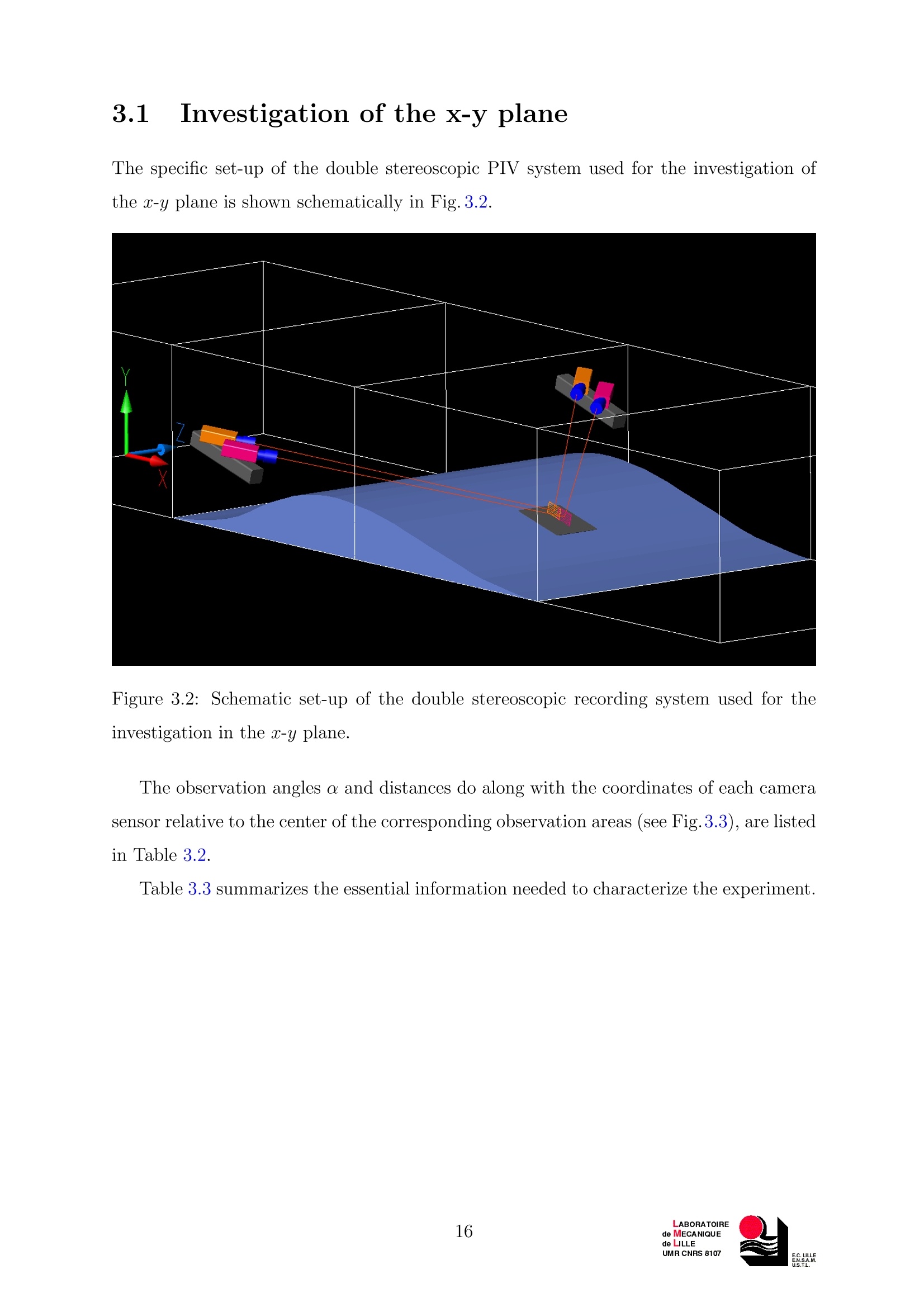
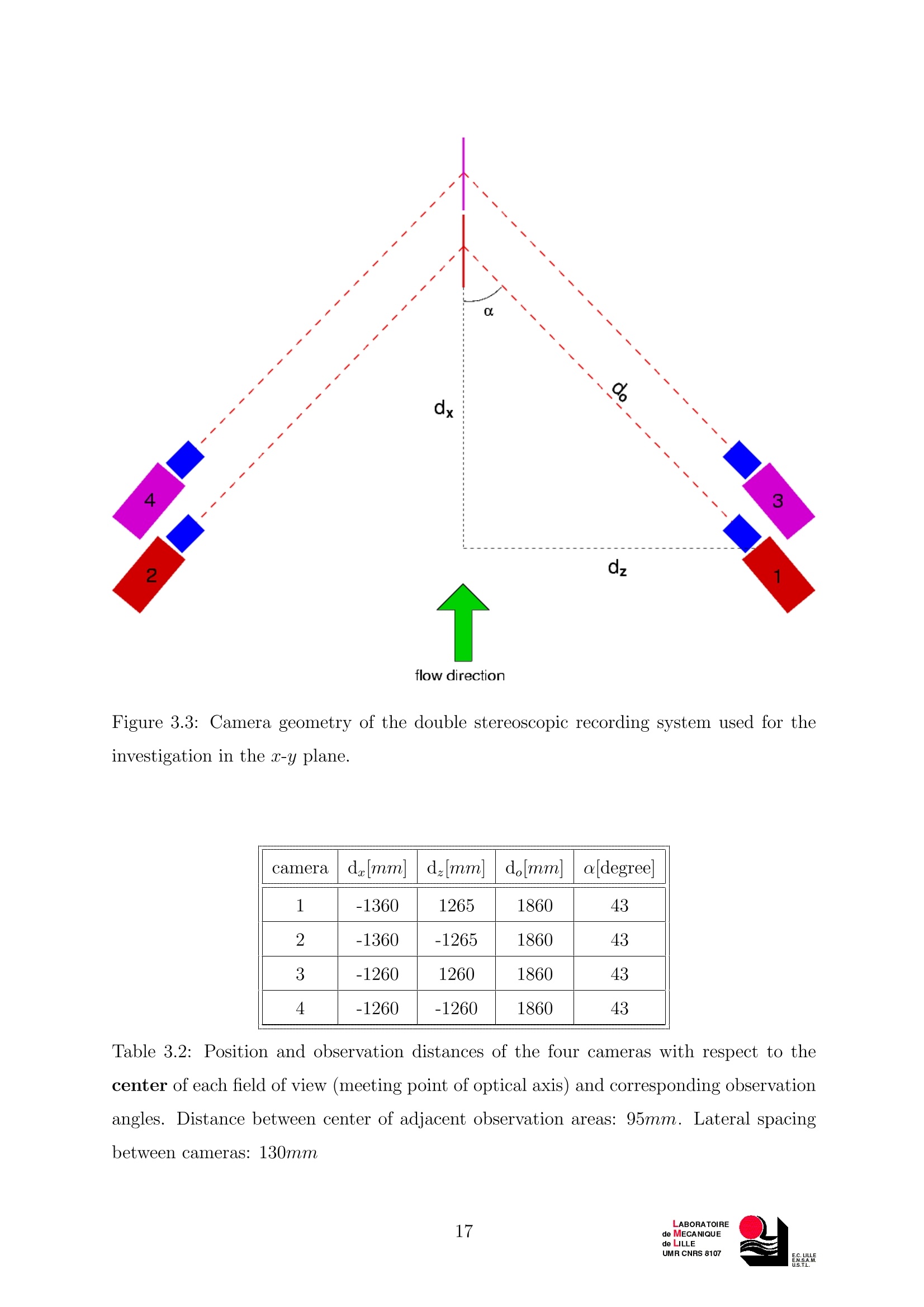
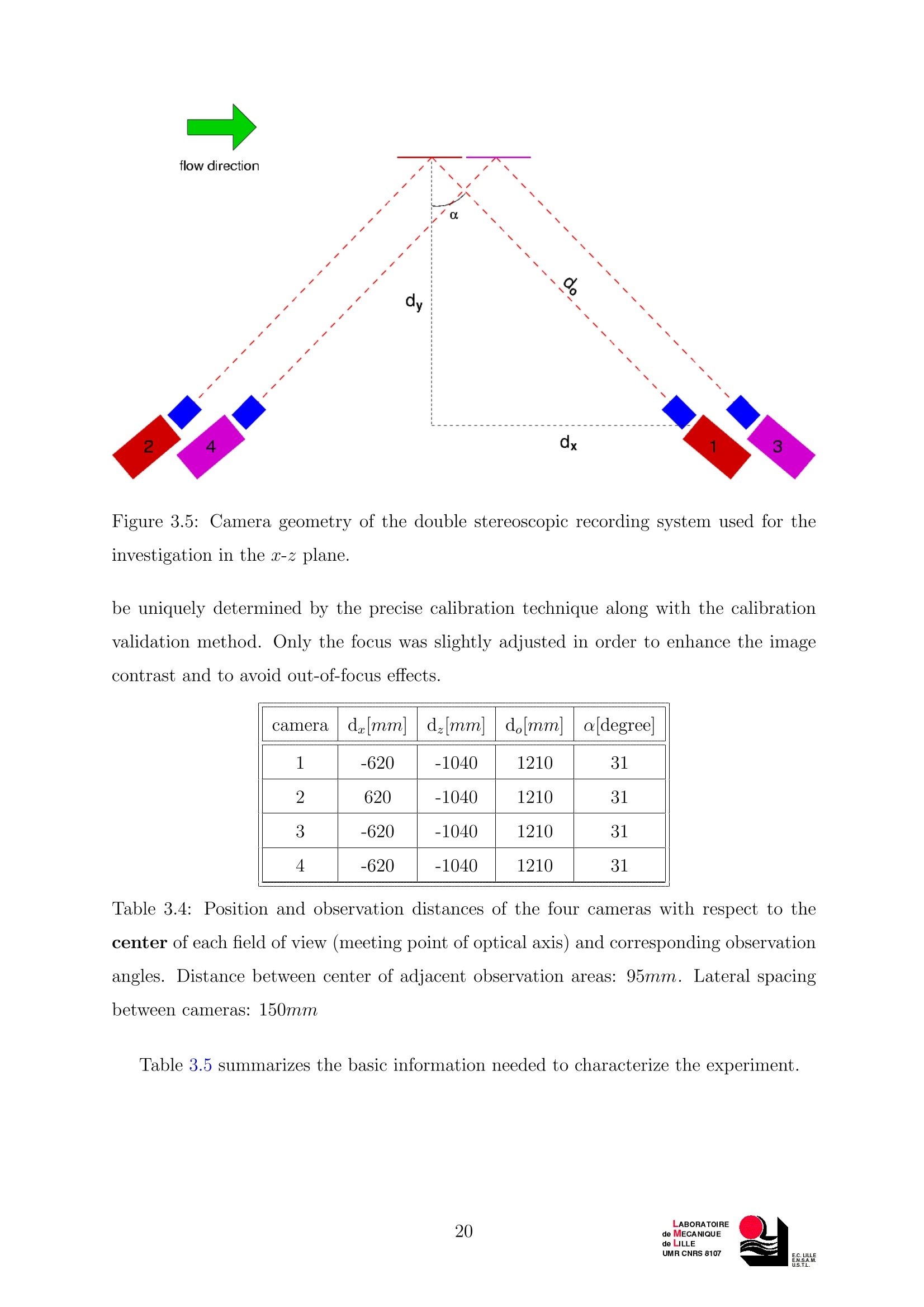
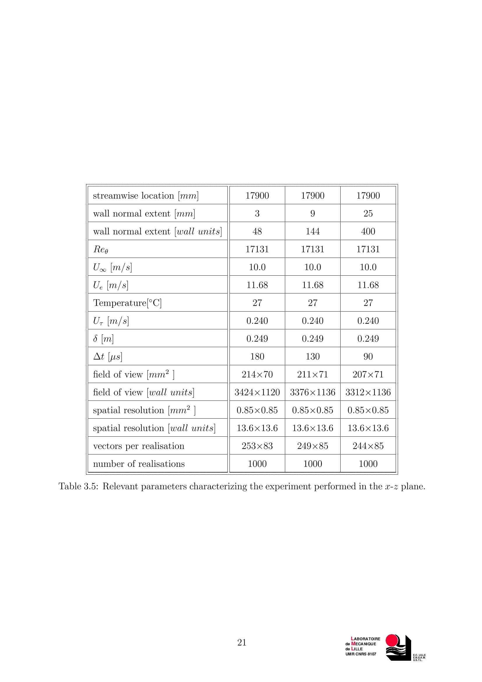
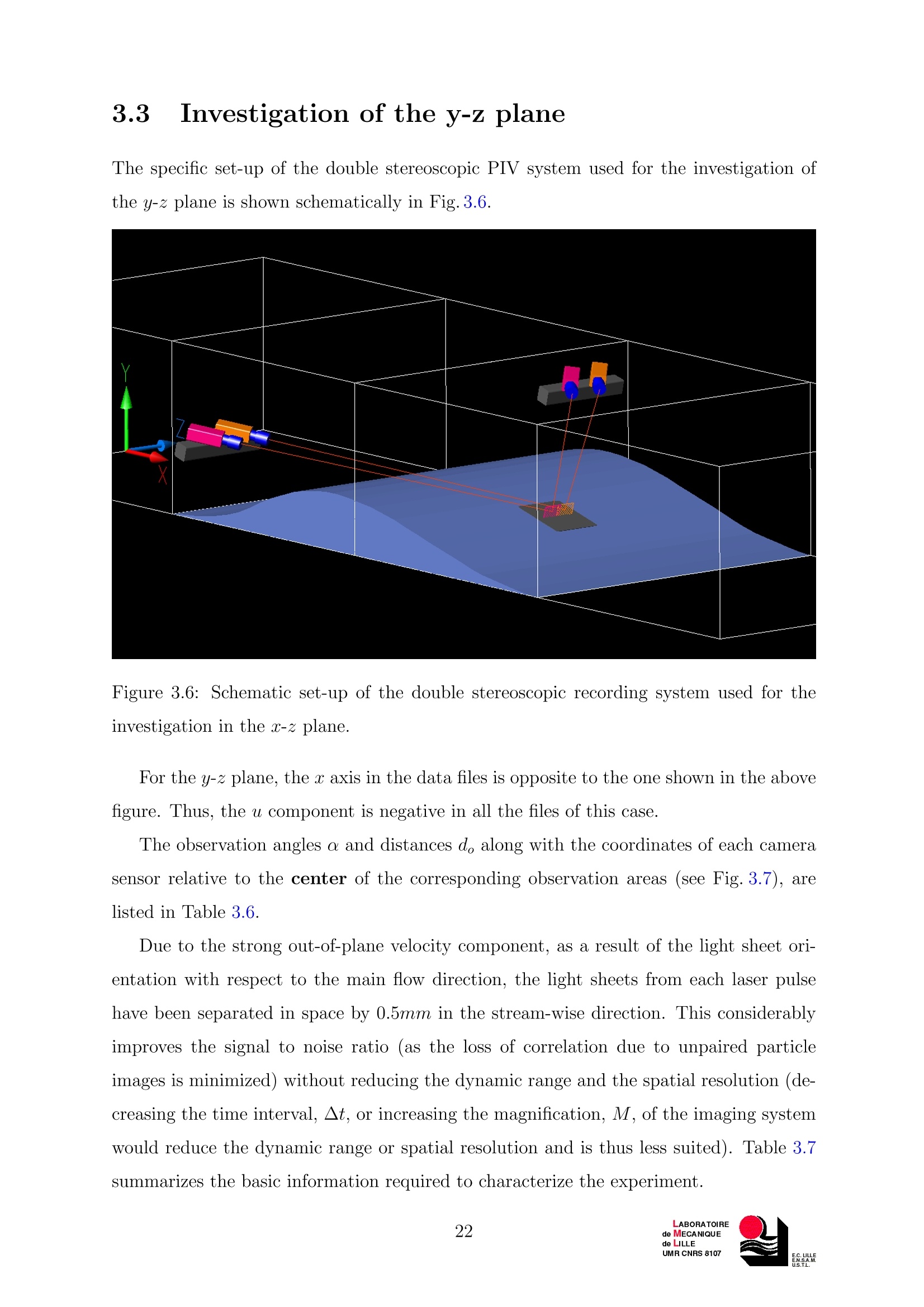
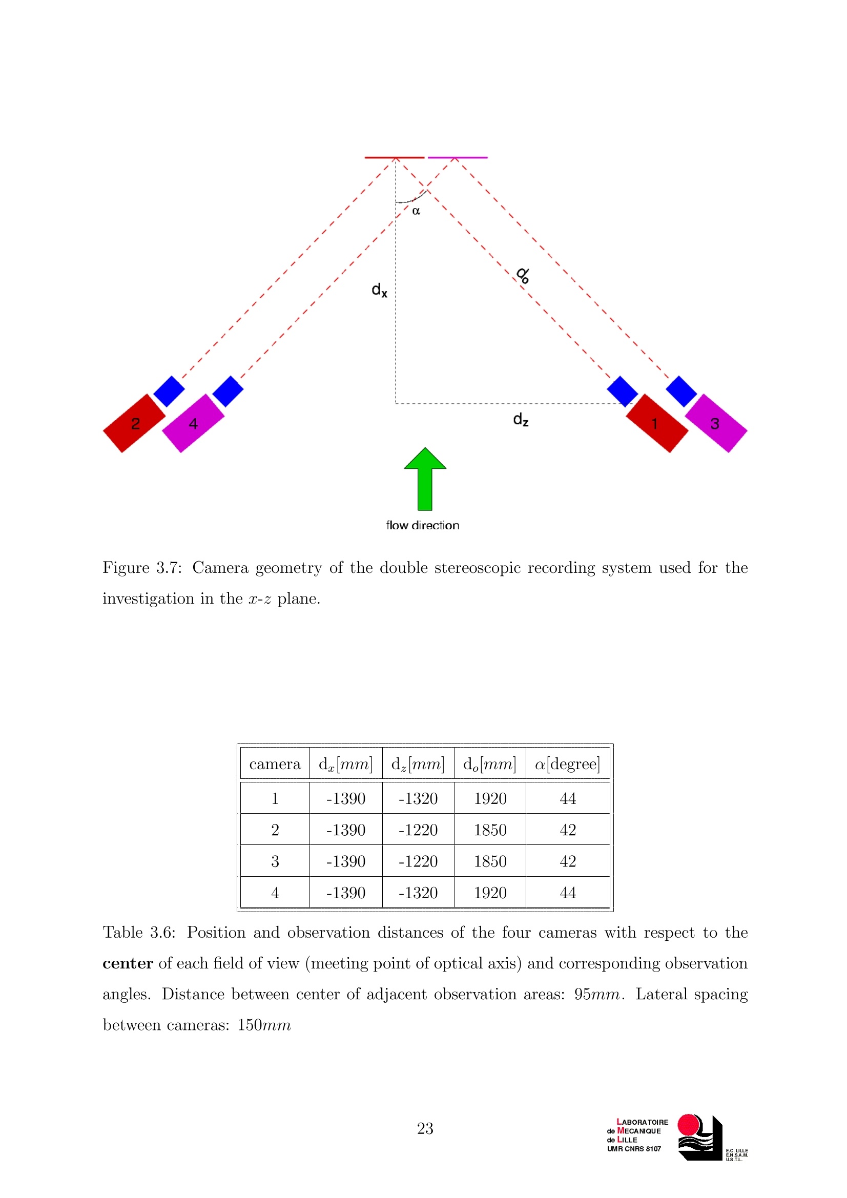
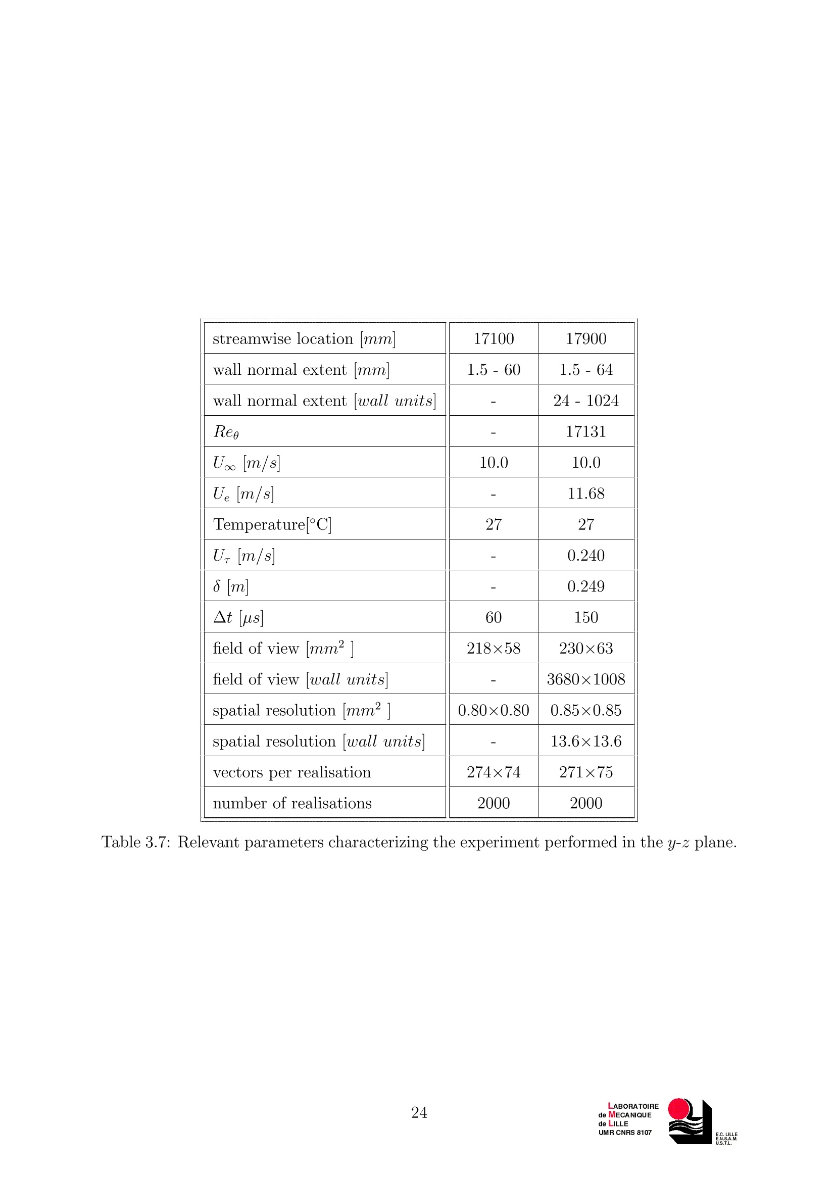
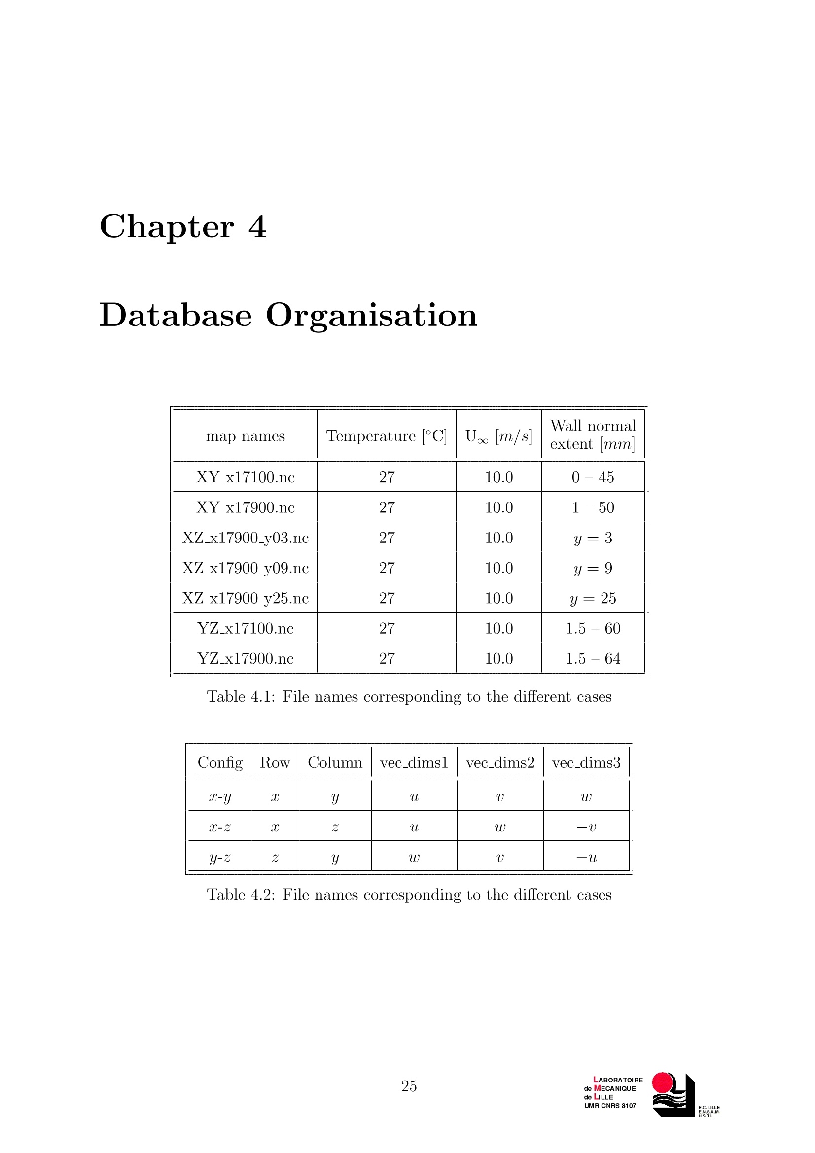
INVESTIGATION OF NEAR WALLTURBULENCE STRUCTURE OF AN APGTBL USING DOUBLE SPIV Correspondants ：Stanislas， M.1 Foucaut， J.M.I Kostas， J. ( Laboratoire de Mecanique de Li l le， UMR CNR S 8107， Boule v ard Paul Langev i n， Cite S c ient i fique，59 655 Villeneuve d'Ascq， F rance ) Contents Nomenclature iii Motivation V 1LExperimental Facility 1 Wind Tunnel 1 APG Turbulent Boundary Layer Flow 3 1.2.1 APG Flow Characterisation 4 2Stereo Particle Image Velocimetry (SPIV) 7 2. Laser system 72 Camera system.. 8 2.3 Stereo image recording 9 2.4 Stereo PIV calibration and processing . 10 3 Experimental Details 13 . IInvestigation of the x-y plane 16 Investigation of the x-z plane 19 Investigation of the y-z plane 22 4Database Organisation 25 Bibliography 26 5GUL Nomenclature Reference frame Longitudinal coordinate y Normal coordinate Transversal coordinate S-y，S-2， y-2 Names of PIV planes corresponding to the principal planes of thereference frame Fluid parameters p Density Kinematic viscosity T lemperature P Pressure u Velocity vector Vorticity vector Wall turbulence parameters UReference velocity External velocity Wall friction velocity Cf Skin friction coefficient H Shape parameter EN.S.A.M Boundary layer thickness * Displacement thickness 0 Momentum thickness Taylor micro-scale Re Reynolds number based on boundary layer thickness Res* Reynolds number based on displacement thickness Re0 Reynolds number based on momentum thickness Re Reynolds number based on Taylor micro-scale 十 Wall unit scaled value (...+=...ur/u) PIV parameters Observation angles of the stereoscopic cameras d. Distance between camera and object plane along the axis d Distance between camera and object plane alongx dy Distance between camera and object plane along y d. Distance between camera and object plane along z ATime interval between laser pulsesAA AA Temporal separation between velocity fields Spatial separation between light sheets along c Spatial separation between light sheets along y Spatial separation between light sheets along z EN.S.A.M Motivation One of the fascinating phenomena of natural science which has gripped the attention ofmany scientists is the problem of turbulence. Besides the ubiquitous variety and beautyof turbulent phenomena， the inherent fascination and attraction are strongly connectedwith the enormous difficulties associated to its physical and mathematical understanding.As a general solution is out of reach， the properties of different idealized flows with simplegeometries are being examined experimentally and numerically. Since its discovery by Prandtl， the boundary layer has been a subject of growing in-terest and is still an active subject of research. Due to both its fundamental and technicalinterest， the fully developed turbulent boundary layer in a nominally zero pressure gradi-ent (ZPG) has been examined extensively. A flow of equal importance and perhaps morewidely observed in practice is the turbulent boundary layer (TBL) in the presence of anadverse pressure gradient (APG). This flow has not received the same attention as theZPG TBL due to its increased complexity and the necessity of firstly understanding theZPG situation. One basic characteristic of turbulence is that it varies in space and time. Thus， toassess its physics in a deterministic approach， one needs to characterize both of theseaspects.. This is possible with a numerical approach (DNS and LES) but requires a highspeed holographic technique， for example， to obtain the same results on the experimentalside， which presently is not technologically feasible. The majority of experimentally gath-ered knowledge on both ZPG and APG TBL’s has been limited by the capabilities of singlepoint measurement probes and flow visualization. The former technique is quantitativebut point wise while the latter is spatial but only qualitative. Standard PIV， despite its limitations (it is 2D2C and not resolved in time) has givennew insight into the spatial and statistical approaches of studying turbulence. The de-velopment of high quality CCD cameras and Nd-YAG lasers over the past 5 years， have provided opportunity for a progressive development of the technique， particularly in ob-taining the third component of the velocity vector via the stereo method. Furthermore，the improvement in the accuracy， spatial resolution and user friendliness of PIV systemsis such that turbulent flow investigations can now be easily conducted. The main attraction of PIV is that by providing both spatial and quantitative (instan-taneous velocity maps) information， it brings a completely new experimental insight intoturbulence. This new approach can be put in parallel with the DNS and LES approacheson the numerical simulation side. For this reason， the Laboratoire de Mecanique de Lille(LML) has performed an experiment in a purposely designed boundary layer wind tunnel.A multi-plane stereo PIV technique was used to investigate the complex spatio-temporalflow structure of wall turbulence and will give access to quantities which are of funda-mental importance for the statistical description of turbulence and the study of coherentstructures. An investigation of the near wall turbulent structure of an adverse pressure gradientturbulent boundary layer was performed usinga 4-camera stereo PIV system. The exper-iment was carried out during August 2004 and April 2005， principally by J.M. Foucaut， J.Kostas and M. Stanislas of LML (Kostas et al.， 2005). The resulting database consists ofPIV measurements performed at Reg= 15000 in all the principal planes of the boundarylayer (a-y，-z， y-z). The present document describes the experimental methodology anddatabase in detail. EN.S.A.M Chapter 1 Experimental Facility 1.1 Wind Tunnel The boundary layer wind tunnel used in the experiments is shown in Figs.1.1 and 1.2.The test section is 1m high， 2m wide and 21.6m long with the last 5m having transparentwalls on all sides to permit the use of optical flow diagnostic techniques.Thanks toits length， this facility allows high resolution experiments at Reynolds numbers up toReg =20000 with a boundary layer thickness of the order of 0.3m in the flat plate case.Additionally， the tunnel’s length ensures disturbances arising from the tripping device arenot statistically detectable in the test section. A large plenum chamber with guide vanesfollowed by a honeycomb， grids and a contraction decreases the turbulence level to about0.7%of the external velocity at the entrance of the wind tunnel. The wind tunnel can be operated in either a closed loop configuration with temperatureregulation or an open loop configuration where it is opened to the atmosphere to allow theuse of smoke. For the present study， the wind tunnel is used in a closed loop configurationwhich allows a finer control of the flow parameters. In this configuration the wind tunnelis computer controlled by a PC， regulating both the velocity and the temperature. An air-water heat exchanger located in the plenum chamber allows the freestream temperatureto be maintained to within ±0.2°C. In the open loop configuration only the velocity isregulated by computer. The velocity in the testing zone can be varied continuously from3m/s to 10m/s with a stability better than ±0.01%. A free-stream velocity of 10m/swas used throughout the experiments in the present investigation. The boundary layer to be studied develops on the lower wall. A grid laid on the lower Figure 1.1： Plan view of the LML wind tunnel. 1 plenum chamber； 2 guide vanes； 3honeycomb； 4 grids； 5 contraction； 6 development zone； 7 testing zone； 8 fan and motor；9 return circuit； 10， air-water heat exchanger. Figure 1.2： Photograph of the LML boundary layer wind tunnel. wall of the tunnel entrance acts as a trip and ensures the boundary layer is turbulent atthe testing zone. The origin of the coordinate system lies in the middle of the lower wallat the entrance of the tunnel with the s axis parallel to the wall and the flow (stream-wise direction)， the y axis normal to the lower wall (wall-normal direction) and the z axisperpendicular to the oncoming flow and parallel to the lower wall (span-wise direction)， see Fig. 1.4. Measurements are conducted in a stationary reference frame relative to theaboratory.Further details about the wind-tunnel and flow characteristics， like shapeparameter， skin friction coefficient and strength of the wake component， can be found inCarlier & Stanislas (2005). 1.2 APG Turbulent Boundary Layer Flow An adverse pressure gradient (APG) is generated using a 2-D bump attached onto thelower wall of the tunnel. It is the same bump used throughout the AEROMEMS project.The shape was computed by Dassault Aviation using a 2-D Navier-Stokes solver with ak-e turbulence model. The objective was to approach separation without reaching it inorder to prevent the flow becoming 3-D. Figure 1.3： Schematic of the bump designed to produce the APG flow. Figure 1.3 illustrates the bump design. It consists of 3 main parts. The first is theconverging part， constructed from 2mm thick steel sheet. A longitudinal adjustment ofthis part of the bump relative to the centre part of the model is possible. ThiTshis centreportion is made from wood covered with a thin steel sheet and is connected to a flataluminium plate further downstream in the divergent part of the bump. Within thisaluminium plate there exists an opening designed to accept models and other measurementdevices (e.g. sensors， glass window，etc.). The third part of the bump consists ofa flexiblesheet of PVC that is shaped to obtain a smooth transition with the wind tunnel floor.The bump surface is painted black and is equipped with pressure taps along the bump’s EN.S.A.M longitudinal centreline. This permits a direct measurement of the stream-wise pressuregradient. A diagram of the bump mounted in the wind tunnel is shown in Fig.1.4. Furtherdetails of the design， manufacturing and mounting of the bump in the wind tunnel maybe found in the AEROMEMS I final report (Bernard et al.， 2000). Details of the flowquality may also be found in the same report and Bernard et al. (2003). Figure 1.4： The wind tunnel and bump in the laboratory reference frame. 1.2.1 APG Flow Characterisation The following well established flow diagnostic techniques were used to characterise theAPG TBL flow ： 1. A single component hot-wire anemometry was used to characterise the basic flow. 2. Surface pressure taps along the centreline of the bump were used to characterise thepressure gradient distribution along the bump. Hot-Wire Anemometrv In the present study， the principal technique for characterising the basic flow was hot-wireanemometry. Only singe wire probes were used. They were manufactured by AUSPEX EN.S.A.M with platinum plated tungsten wire 2.5um in length. They were mounted on a computercontrolled traversing system which allowed them to be positioned to within 0.2mm ofthe wall. The traversing system was adjusted normal to the wall at each measurementstation. Calibration was performed at the mid-height of the wind tunnel， in a regionwhere the velocity profile was uniform. The probes were connected to a four channelAN-1003 AAlab hot-wire anemometer whose signal was low-pass filtered at 5.5kHz anddigitized by a personal computer equipped with an A/D converter board and a sampleand hold circuitt..TIhe acquisition frequency was 11kHz and 1.1 × 10° samples weretaken at each measurement location. Calibration and measurements were fully computercontrolled， with temperature and velocity regulation present for each. The temperaturewas the same for the calibration and the measurements. Five streamwise stations werechosen to characterise the flow.. The streamwise coordinate x = 17.0m corresponds tothe top of the bump. The results are presented in Table 1.1. Further details of the flowcharacterisation may be found in Bernard et al. (2003). X，m Parameter 17.35 17.63 17.90 18.24 18.58 s， m 0.350 0.640 0.918 1.267 1.611 Ue， m/s 13.61 12.53 11.68 10.88 10.56 8，m 0.115 0.188 0.249 0.364 0.455 8*， m 0.0066 0.0169 0.0329 0.0618 0.0782 0，m 0.0053 0.0128 0.0224 0.0363 0.0462 8**，m 0.0099 0.0234 0.0396 0.0662 0.0784 H12 1.24 1.319 1.471 1.703 1.693 H32 1.858 1.820 1.772 1.715 1.697 H 1.18 1.05 0.95 0.87 0.85 Cf 0.0031 0.0017 0.0008 0.0003 0.0005 Ur，m/s 0.535 0.365 0.240 0.140 0.165 Reg 4，887 10，501 17，131 26，112 32，384 Reo 5，988 14，117 25，618 44，825 55，052 8+ 4，293 5，765 4，399 4，975 5，308 p+ 0.0064 0.0216 0.0518 0.1376 0.0373 1.51 8.89 27.27 79.35 32.07 0.059 0.259 0.560 1.021 0.501 Table 1.1： Global characteristics of the APG TBL (Bernard et al.，2003). Pressure Measurements Detailed pressure measurements were performed to characterise the pressure distributionand to ensure its two dimensionality. A series of pressure taps along the centreline of the bump were connected to a Furness FC014 micro-manometer pressure transducer whichhad a full measurement range of 10-mm H20. The accuracy of these measurements was±0.1Pa. The the streamwise distribution of the pressure coefficient along the bump couldthus be determined. The upstream outer velocity was used as the reference. The measured streamwise distribution of C，as compared to the predictions obtained byDassault Aviation using a 2-DNavier-Stokes solver with a k-e turbulence model is shownin Fig.1.5. Figure 1.5： Measured pressure distribution along the centreline of the bump (Bernardet al.，2003). Chapter 2 Stereo Particle Image Velocimetry(SPIV) A multi-plane， multi-camera， stereo PIV technique was used in the present study toacquire planar velocity fields in the x-y， s-z and y-zplanes of the flow. This technique isreliable， robust and relatively easy to implement. It is based on standard PIV equipmentand evaluation procedures， so that available PIV systems can be easily extended. It makespossible the measurement of all three velocity components in a plane and has been shownin various experiments to be well suited for measuring， with high accuracy， a variety offundamentally important fluid mechanical quantities. The multi-plane stereo PIV system consists of a two pulse laser system delivering twoidentically polarized pulses， two pairs of high resolution progressive scan CCD cameras inan angular imaging configuration with Scheimpflug correction and an appropriate combi-nation of optics to generate a light sheet at the measuring location. Particle seeding isachieved with commercially available smoke generators placed just upstream of the faninlet. 2.1 Laser system The LML laser system used was a BMI PVL special series 5000 with four cavities. Theoutput energy is approximately 300mJ per pulse， per cavity at a wavelength of 532nm.The pulse repetition frequency is adjustable between 10Hz and 15Hz. The laser can beoperated in either a 4 oscillator mode or a 2 oscillator， 2 amplifier mode (which effectively EN.S.A.M Type BMI special series 5000 Number of cavities 4 Lasing material Nd：YAG Transversal mode TEM00 Pulse durationns <5 Output energy perpulse mJ 0-600 Frequency [Hz] 10-15 Table 2.1： Main characteristics of LML laser system. doubles the energy output per pulse， but yields a poorer beam quality). For the currentset of experiments， the laser was operated in the 4 oscillator mode as there was sufficientlight available and the beam quality was considerably better than for the 2 oscillator， 2amplifier mode. An appropriate combination of cylindrical and spherical lenses was used to form alight sheet approximately 0.5mm thick and 0.5m wide at the measurement location (seeFig. 2.1). The light sheet was directed towards the test-section with high energy mirrorsoptimised for 532nm. All these elements could be rotated and translated to adjust thelaser sheet in the selected plane. 2.2 Camera system Four Peltier cooled high resolution digital cameras were used to record the particle images.They have a progressive scan sensor technology combined with a low read-out noise of thecamera-interface board yielding a high signal to noise ratio. Each camera was capable ofacquiring images in cross-correlation mode (with an inter-frame time as small as 500ns)with a 12 bit dynamic range. In the present experiment， an acquisition frequency of 4Hzfor double image acquisition was utilised. The field of interest was imaged using f#4200mm and f#2.8 105mm Micro Nikkor lenses. The aperture was adjusted from f#5.6to f#16 in order to adjust the depth-of-focus and to minimize the optical aberrationsintroduced by the 10mm glass-walls of the wind-tunnel. Each camera was connected to aScheimpflug adapter in order to precisely adjust the angle between the image， object andmain plane of the lens so that a uniformly focused image resulted. ENS.A.M Type LaVision Sensicam LaVision ImagerIntense Pixel numberpicels 1280×1024 1376×1040 Pixel size [[um21 6.7×6.7 6.4×6.4 Sensor size[mm21 8.6×6.9 8.8×6.7 Sensor temperatureC -12 -12 Dynamic range bits 12 12 Frequency.[Hz] 8 10 Transfer interline interline Table 2.2： Main characteristics of cameras. The entire wind tunnel was seeded using a commercially available smoke generator.This produced a high concentration of mono-disperse poly-ethylen-glycol (PEG) tracerparticles with a mean diameter of the order of 1um. Seeding inhomogeneities quicklydisappeared due to mixing after the smoke had completed several circuits of the windtunnel. Any diffuse wall reflections were removed by cleaning the tunnel windows withappropriate liquids and pressurized air while the wind-tunnel was operating at a moderatespeed. 2.3 Stereo image recording The particle images are recorded by means of the CCD cameras in an angular imagingconfiguration. The camera positions were adjusted to try to maximise the angle betweenthem， whilst still achieving an unobstructed field of view. The four cameras were mountedon an extruded aluminium beam support that was tilted to the horizontal so that it wasparallel to the bump surface at the observation region. The resulting stereo PIV layout wassymmetrical about a line perpendicular to the bisector of the field of view (see Fig.2.1). Due to the oblique viewing direction and the limited depth of focus of the lens， theimage plane， the main plane of the lens and the object plane need to intersect along a com-mon line (Scheimpflug condition) in order to obtain focused particle images everywherewithin the image plane. Therefore， each camera lens must be connected to a specially de-signed Scheimpflug-adapter. The axis of rotation coincides with the centerline of the CCDsensor to ensure that all particle images along this axis remain in focus under rotation. This simplifies the installation of the system and the focusing process since the imagelocation of the centerline in object space and the opening angle between correspondingcamera pairs remains constant under Scheimpflug angle adjustment.. jFor magnificationand field of view adjustments (necessary for maximizing the amount of stereo informa-tion) all Scheimpflug-adapters are mounted on a two-axis linear translation stage whichallows high precision translations by thumb screws. In order to simplify the adjustmentprocedure without restricting the flexibility of the system the left and right recordingsystems can be connected to different base-plates with individual rotation stage. Unfortunately， the Scheimpflug condition has the side effect of introducing a strongperspective distortion which has to be carefully determined to ensure that the interroga-tion windows from each pair of stereoscopic records correspond to the same flow regionsand the magnification is constant for all image positions. 2.4 Stereo PIV calibration and processing In order to extract the third velocity component with any degree of accuracy from thestereoscopic images of each camera pair， the stereo PIV system must first be calibrated. Geometric back projection based on geometric optics can be used. However， it requiresexact knowledge of the imaging parameters such as the lens focal length， the anglesbetween the various planes and the nominal magnification factor. The geometric opticexpressions do not incorporate non-linearities such as lens distortions and are sensitiveto small variations in each parameter. A more robust method is the warping approachincorporating the Soloff technique (Soloff et al.， 1997)， which is used here. This techniquehas the advantage of performing back-projection and stereo reconstruction in a single stepwith the further advantage of not requiring any knowledge of geometrical parameters ofthe optical arrangement which can be prone to measurement inaccuracies hence affectingthe reconstruction. A calibration plate consisting of a regular array of accurately positioned markers (inthis case cross markers) is aligned so that it coincides as close as possible with the centerof the light sheet plane. To facilitate this it was glued onto a flat aluminium plate， whichwas itself attached to a 3-axis micrometer translation stage. This ensured a very accuratepositioning and movement of the grid in the desired direction. Once the calibration plate (a) (c) Figure 2.1： Laser sheet and camera orientations for recording of the various measurementplanes. (a) s-y plane， (b) ac-z plane and (c) y-z plane. was precisely aligned with each light sheet its image was recorded at a number of planestranslated in the out of plane direction (including the zero position) with each of the fourcameras. A projection function can then be determined that allows one to map each pointwithin the deformed image plane to the undeformed object plane， where the magnificationfactor is constant across field of view. Simplified stereoscopic equations can then be applied to calculate a 2D3C velocity fieldfrom a pair of 2D2C velocity fields since the magnification factor is now constant. In thecurrent set of measurements stereoscopic reconstruction of the three velocity componentswas performed using a 3 plane Soloff analysis. The local misalignment between the the laser sheet and the calibration grid arisingfrom imprecise placement of the target can be accounted for by using the method of(Coudert & Schon， 2001). By performing a cross-correlation analysis between the de-warped images acquired at the same time from each camera pair a displacement fieldcorresponding to the misalignment (translation， rotation or deformation) can be deter-mined. This can then be used to correct the vector field calculated with the misalignedgrid. The particle image processing was performed using the PIVGML software developed atLML. The images from each camera were processed with a standard multi-grid algorithmWwith discrete window offset. The final interrogation window size was 32 × 32 picelswith 50% overlap. For sub-pixel accuracy two 1-D Gaussian fits in two directions wereused to determine the position of the correlation peak. The final size of the interrogationwindows was 32×32 pixels with an overlapping of 50%. EN.S.A.M Chapter 3 Experimental Details The experiments were performed at a nominal tunnel velocity of U..= 10m/s. In allcases the two camera systems were adjusted so that the corresponding velocity maps wereadjacent to one another. This was done in order to extend the field of view whilst retaininga good spatial resolution required for investigating the turbulent structures. The fields ofview of each camera pair were slightly overlapped with one another to ensure continuityof data throughout the extent of the entire image region.The temporal and spatialseparations between the velocity maps (Ar and▲x， Ay， Az respectively) were all zerofor each measurement orientation. The time interval between laser pulses， At， was chosen as a compromise between max-imising the dynamic range of the measurement (i.e. maximising the particle displace-ment) and ensuring particles remained within the light sheet during this time period， thusyielding a high success rate of particle image correlations during the PIV analysis. Thepulse separation times chosen， yielded a nominal particle displacement of approximately10pisels. The synchronisation of laser pulses and cameras， timing control and image ac-quisition were performed with the LaVision Da Vis PIV software and computer hardware.Image sets were stored directly to hard disk during acquisition. They were then archivedonto DVD for future processing. Measurements were conducted in all the principal planes of the boundary layer， x-y，x-z， and y-z. Two streamwise locations were measured for the s-y and y-z planes whilethe presence of only one optical access window on the bump restricted measurements toone streamwise location for the a-z plane. Three plane heights were measured for the xc-zplane. The furthest from the wall corresponded to the peak in turbulence intensity which Measurementconfiguration tunnel referencevelocitym/s Number ofmeasured planes Number of realisationsper plane -y 10 1 2000 C-Z 10 3 1000 y-2 10 1 2000 Table 3.1： Measurements conducted for each configuration. had been established from the hot-wire measurements. The location of the measurementplanes is illustrated in Fig.3.1. A large number of statistically independent realisations were acquired for each dataset.This ensured acceptably converged turbulence statistics. Two thousand vector field real-isations were acquired for each of the s-y and y-z planes， while one thousand vector fieldrealisations were acquired for each wall height measured in the s-z plane. Measurements at each location were non-dimensionalised with respect to the localexternal velocity， Ue and the local wall friction velocity， ur. Physical limitations preventedthe measurement of the external velocity and wall shear stress at the s =17.100m location.Therefore the information characterising the experiment and the data itself was not non-dimensionalised at this streamwise location. EN.S.A.M Wall Figure 3.1： Location of the various measurement planes (MP’s). (a) ax-y plane， (b) -zplane and (c) y-z plane. 3.1 Investigation of the x-y plane The specific set-up of the double stereoscopic PIV system used for the investigation ofthe a-y plane is shown schematically in Fig.3.2. Figure 3.2： Schematic set-up of the double stereoscopic recording system used for theinvestigation in the c-y plane. The observation angles a and distances do along with the coordinates of each camerasensor relative to the center of the corresponding observation areas (see Fig.3.3)， are listedin Table 3.2 Table 3.3 summarizes the essential information needed to characterize the experiment. Figure 3.3： Camera geometry of the double stereoscopic recording system used for theinvestigation in the -y plane. camera drmm dzmm dmm o degree 1 -1360 1265 1860 43 2 -1360 -1265 1860 43 3 -1260 1260 1860 43 4 -1260 -1260 1860 43 Table 3.2： Position and observation distances of the four cameras with respect to thecenter of each field of view (meeting point of optical axis) and corresponding observationangles. Distance between center of adjacent observation areas： 95mm. Lateral spacingbetween cameras： 130mm EN.S.A.M streamwise locationmm 17100 17900 wall normal extentmm 0-45 1-50 wall normal extentwall units - 16-800 Reo 17131 U.。m/s 10.0 10.0 Uem/s 一 11.68 TemperatureC 27 27 Um/s - 0.240 5[m] - 0.249 At us 30 70 field of view r[mm²1 152×45 195×49 field of viewwall units - 3120×784 spatial resolution [mm²1 0.75×0.75 0.85×0.85 spatial resolutionwall units - 13.6×13.6 vectors per realisation 204×62 230×59 number of realisations 2000 2000 Table 3.3： Relevant parameters characterizing the experiment performed in the s-y plane. C.4 3.2 Investigation of the x-z plane The specific set-up of the double stereoscopic PIV system used for the investigation ofthe s-z plane is shown schematically in Fig. 3.4. Figure 3.4： Schematic set-up of the double stereoscopic recording system used for theinvestigation in the c-z plane. The observation angles a and distances do along with the coordinates of each camerasensor relative to the center of the corresponding observation areas (see Fig. 3.5)， for theplane y=9mm， are listed in the Table 3.4. Mounting the light sheet generating optics before the final 90 degree mirror (whichwas itself mounted onto a linear traversing stage) allowed a relatively easy adjustment ofthe light sheet height above the bump surface. It was important to ensure the light sheetwas parallel to the bump surface. This was checked by measuring the light sheet heightrelative to a fixed reference point on the tunnel frame on entering and exiting the workingsection. The light sheet height above each end of the bump window was also checked. Anangle of no more than 0.1 degrees was considered acceptable across the bump window. Due to the small spatial separation between the different light-sheet planes it was notnecessary to move any camera when changing measurement position as all effects could EN.S.A.M Figure 3.5： Camera geometry of the double stereoscopic recording system used for theinvestigation in the s-z plane. be uniquely determined by the precise calibration technique along with the calibrationvalidation method. Only the focus was slightly adjusted in order to enhance the imagecontrast and to avoid out-of-focus effects. camera dr mm dzmm dmm a degree 1 -620 -1040 1210 31 2 620 -1040 1210 31 3 -620 -1040 1210 31 4 -620 -1040 1210 31 Table 3.4： Position and observation distances of the four cameras with respect to thecenter of each field of view (meeting point of optical axis) and corresponding observationangles. Distance between center of adjacent observation areas： 95mm. Lateral spacingbetween cameras： 150mm Table 3.5 summarizes the basic information needed to characterize the experiment. streamwise locationmm| 17900 17900 17900 wall normal extentmm 3 9 25 wall normal extentwall units 48 144 400 Ree 17131 17131 17131 U.。m/s 10.0 10.0 10.0 U m/s 11.68 11.68 11.68 TemperatureC 27 27 27 U， m/s 0.240 0.240 0.240 5[m] 0.249 0.249 0.249 At us] 180 130 90 field of view[mm²1 214×70 211×71 207×71 field of viewwall units 3424×1120 3376×1136 3312×1136 spatial resolution [mm²] 0.85×0.85 0.85×0.85 0.85×0.85 spatial resolution twall units 13.6×13.6 13.6×13.6 13.6×13.6 vectors per realisation 253×83 249×85 244×85 number of realisations 1000 1000 1000 Table 3.5： Relevant parameters characterizing the experiment performed in the x-z plane. 3.3 Investigation of the y-z plane The specific set-up of the double stereoscopic PIV system used for the investigation ofthe y-z plane is shown schematically in Fig. 3.6. Figure 3.6： Schematic set-up of the double stereoscopic recording system used for theinvestigation in the s-z plane. For the y-z plane， the a axis in the data files is opposite to the one shown in the abovefigure. Thus， the u component is negative in all the files of this case. The observation angles a and distances d， along with the coordinates of each camerasensor relative to the center of the corresponding observation areas (see Fig. 3.7)， arelisted in Table 3.6. Due to the strong out-of-plane velocity component， as a result of the light sheet ori-entation with respect to the main flow direction， the light sheets from each laser pulsehave been separated in space by 0.5mm in the stream-wise direction. This considerablyimproves the signal to noise ratio (as the loss of correlation due to unpaired particleimages is minimized) without reducing the dynamic range and the spatial resolution (de-creasing the time interval， ▲t， or increasing the magnification， M， of the imaging systemwould reduce the dynamic range or spatial resolution and is thus less suited). Table 3.7summarizes the basic information required to characterize the experiment. EN.S.A.M Figure 3.7： Camera geometry of the double stereoscopic recording system used for theinvestigation in the a-z plane. camera da mm dz[mm] d.mm o degree 1 -1390 -1320 1920 44 2 -1390 -1220 1850 42 3 -1390 -1220 1850 42 4 -1390 -1320 1920 44 Table 3.6： Position and observation distances of the four cameras with respect to thecenter of each field of view (meeting point of optical axis) and corresponding observationangles. Distance between center of adjacent observation areas： 95mm. LIateral spacingbetween cameras： 150mm EN.S.A.M streamwise location.mm 17100 17900 wall normal extentmml 1.5-60 1.5-64 wall normal extentwall units 一 24-1024 Reo - 17131 U.。m/s 10.0 10.0 Uem/s - 11.68 Temperature°C 27 27 U， m/s - 0.240 m - 0.249 it us 60 150 field of view[mm²1 218×58 230×63 field of viewwall units - 3680×1008 spatial resolutio1n[mm²1 0.80×0.80 0.85×0.85 spatial resolutionwall units 二 13.6×13.6 vectors per realisation 274×74 271×75 number of realisations 2000 2000 Table 3.7： Relevant parameters characterizing the experiment performed in the y-z plane. sC.W Chapter 4 Database Organisation map names Temperature C U.o m/s Wall normalextentmml XY_x17100.nc 27 10.0 0-45 XYx17900.nc 27 10.0 1-50 XZ_x17900_y03.nc 27 10.0 y=3 XZ_x17900_y09.nc 27 10.0 y=9 XZ_x17900_y25.nc 27 10.0 y= 25 YZx17100.nc 27 10.0 1.5-60 YZx17900.nc 27 10.0 1.5-64 Table 4.1： File names corresponding to the different cases Config Row Column vec_dimsl vec_dims2 vec_dims3 c-y y W XC-Z -U y-z y W U 一u Table 4.2： File names corresponding to the different cases EN.S.A.M Bibliography BERNARD， A.， DUPONT， P.， FOUCAUT， JJ.， & STANISLAS，， M. (2000). Identifi-cation and assessment of flow actuation and control strategies. Technical ReportFREP/CN18/MS001101 CNRS-DR18. BERNARD， A.， DUPONT， P.， FOUCAUT， J.， & STANISLAS， M. (2003). Deceleratingboundary layer： a new scaling and mixing length model. AIAA J. 41(2)， 248-255. CARLIER， J. & STANISLAS， M. (2005).E xIperimental study of eddy structures in aturbulent boundary layer using particle image velocimetry. J. Fluid Mech. 535， 143-S—188. COUDERT， S. & SCHON， J. (2001). Back-projection algorithm with misalignment cor-rections for 2D3C stereoscopic PIV. Meas. Sci. Technol. 12， 1371-1381. ( KOsTAS， J .，FOUCAUT， J.， & STANISLAS， M.(20 0 5). Ap p lication of double SPIV on the near wall turbulence structure of an a dverse pressure gradient turbulent b o undarylayer. In 6th International Symposium on PI V Pas a dena， Cali f ornia. ) SOLOFF， S.， ADRIAN， R.， & LIu， Z. (1997). Distortion compensation for generalizedstereoscopic particle image velocimetry. Meas. Sci. Technol. 8， 1441-1454. E.N.S.A.M LABORATOIREde MECANIQUEde LILLEUMR CNRS i