


方案详情
文
The aim of this work was to understand the physical requirements as well as to develop
methodology required to employ Time Resolved Digital Particle Image Velocimetry
(TRDPIV) for measuring high speed, high magnification, near wall flow fields. Previous
attempts to perform measurements such as this have been unsuccessful because of
both limitations in equipment as well as proper methodology for processing of the data.
This work addresses those issues and successfully demonstrates a test inside of a
transonic turbine cascade as well as a high speed high magnification wall jet.
From previous studies it was established that flow tracer delivery is not a trivial task in a
high speed high back pressure environment. Any TRDPIV measurement requires
uniform spatial seeding density, but time-resolved measurements require uniform
temporal seeding density as well. To this end, a high pressure particle generator was
developed. This advancement enhanced current capability beyond what was previously
attainable. Unfortunately, this was not sufficient to resolve the issue of seeding all
together, and an advanced data reconstruction methodology was developed to
reconstruct areas of the flow field that where lost do to inhomogeneous seeding. This
reconstruction methodology, based on Proper Orthogonal Decomposition (POD), has
been shown to produce errors in corrected velocities below tradition spatial techniques
alone. The combination of both particle generator and reconstruction methodology was
instrumental for successfully acquiring TRDPIV measurements in a high speed high
pressure environment such as a transonic wind tunnel facility.
This work also investigates the development of a turbulent wall jet.
方案详情

By Samuel G.Raben Thesis submitted to the Faculty of the Virginia Polytechnic Institute and State Universityin Partial Fulfillment of the Requirements for the Degree of Master of Science In Mechanical Engineering Dr. Pavlos P. Vlachos Co-chairman Dr. Wing F. Ng Co-chairman Dr. Karen A. Thole Dr. Kenneth S. Ball April 28*,2008 Blacksburg, Virginia Keywords: Particle Image Velocimetry, Proper Orthogonal Decomposition, DataReconstruction, Wall Jet, High Magnification, Near Wall Copyright 2008, Samuel G. Raben By Samuel G. Raben (ABSTRACT) The aim of this work was to understand the physical requirements as well as to developmethodology required to employ Time Resolved Digital Particle Image Velocimetry(TRDPIV) for measuring high speed, high magnification, near wall flow fields. Previousattempts to perform measurements such as this have been unsuccessful because ofboth limitations in equipment as well as proper methodology for processing of the data.This work addresses those issues and successfully demonstrates a test inside of atransonic turbine cascade as well as a high speed high magnification wall jet. From pre)vrieovuIsO UsSt:udies it was established that flow tracer delivery is not a trivial task in ahigh speed high back pressure environment.L.Any TRDPlV measurement requiresuniform spatial seeding density, but time-resolved measurements require uniformtemporal seeding density as well. To this end, a high pressure particle generator wasdeveloped. This advancement enhanced current capability beyond what was previouslyattainable. Unfortunately, this was not sufficient to resolve the issue of seeding alltogether, and an advanced data reconstruction methodology was developed toreconstruct areas of the flow field that where lost do to inhomogeneous seeding. Thisreconstruction methodology, based on Proper Orthogonal Decomposition (POD), hasbeen shown to produce errors in corrected velocities below tradition spatial techniquesalone. The combination of both particle generator and reconstruction methodology wasinstrumental for successfully acquiring TRDPIV measurements in a high speed highpressure environment such as a transonic wind tunnel facility. This work also investigates the development of a turbulent wall jet. This experimenthelped in demonstrating the capability of taking high speed high magnification TRDPIVmeasurements.This experiment was very unique in that it is one of only a fewexperiments that studied the developing region of these jets. The Reynolds numberranged for this experiment from 150-10,000 which corresponded to velocities of 1 -80m/s. The results from this experiment showed good agreement with currently publishedtime averaged data. Using scaling laws for fully developed jets a new scaling law wasfound for the developing region of the jet that could be applied to all Reynolds numbersin this study. A temporal investigation was also carried out using the temporalcoefficients from POD. A vortex identification scheme was also applied to all of theReynolds numbers showing clear trends as Reynolds number increased. This work is dedicated to the Memory of Patrick Leung.Forever in our memories. l would like to first thank my parents for their love and for supporting both my academicas well as my many extracurricular activities.. While working together was not alwayseasy they never let me give up and that, in large part, is why I am here today. I want tothank my little brother for our countless conversations that keep me thinking, like what’smy favorite math equation. I would also like to thank Jaime for her love and support.Without youI would be lost. I want to thank my cat Riot for waking me up bright andearly so thatI can get into the lab and get lots of work done. I want to thank mycommittee:Dr. Vlachos for taking a chance on me and helping me into graduate school,Dr. Ng for lending his time as well as recourses to help further my education, Dr. Tholeyour example of excellence has had a strong effect on me, Dr. Ball for making time towork with me as his schedule is nothing short of packed. I would also like to thank all ofmy lab mates in AEThER Lab. I would also like to thank so of those I have worked within other labs: Steve, Trey, and Shakeel. I would also like to thank Mike “Rockstar”Ruocco for giving me all too good reasons to take off and take a stress break. Youhave been like a brother to me and I will never forget the times we have had and lookforward to the times we will. I also thank all of those that have come and gone or that Ihave forgotten. TABLE OF CONTENTS .Table of Contents.5.. .iv Table of Figures .. .VI Table of Tables . ..X 1. Gappy Data Reconstruction:..mm 1 1.A. Introduction:mm m 1 1.B. Nomenclature:. 2 1.C. Proper Orthogonal Decomposition and Reconstruction Methodology:..... 2 1.C.IDNS Data and Data Removal:. 2 1.C.II Proper Orthogonal Decomposition: . 3 1.C.IIIEverson-Sirovich Method. 4 1.C.IV Venturi-Karniadakis Method.mmm 5 1.D. Convergence Criteria .... 6 1.D.i Everson - Sirovich Method . 6 1.D.II Venturi -Karniadakis Method. 6 .1.D.IIl Continuity Based Convergence Criteria (CBCC).).. 8 1.E.Results 9 1.E.I Gappy Percentage and Size Resultss. 9 1.E.Il Field Error Analysis.. 13 1.F. Application to Experimental Data.. 16 1.F.I.Experimental Setup.. 16 1.F.II. Results. 18 .1.G Conclusions . .22 2. Wall Jet.... 23 2.A. Introduction 23 2.B. Nomenclature..... 24 2.C. Experimental Setup. 25 2.D. Proper Orthognal Decomposition...... .26 2.E. Vortex Identification. 29 2.F. Results and Discussion .mm. 29 2.F.I Time Averaged Analysis 29 2.F.II Proper Orthogonal Decomposition:.. 33 2.F.III Vortex Identification on POD Reduced Fields. 37 2.G. Conclusion... 38 3. References: 40 Appendix A: Low Speed Cascade Test.. m-44 A.1.Introduction .mm 44 A.2. Nomenclature... 44 A.3. Experimental Methodology....... 45 A.3.i Experimental Facility..... 45 A.3.Il Instrumentation. 47 A.3.III Inlet and Test Conditions .mmi 48 A.4 Results 48 A.5 References. 56 TABLE OF FIGURES Figure 1. The Four stages of the data reconstruction: a) True field, b) Gaps are createdin field, c) A mask is created of all of the gappy locations, d) The field is reconstructed.using the Venturi-Karniadakis method.. 3 Figure 2. Convergence for E-S method determined by equation 9. The arrow denotesthe maximum mode number... 7 Figure 3. Demonstration of the V-K convergence method or 11% 3x3 gappy DNS data.The arrow locates the deviation from the ‘True'spectrum.... 7 Figure 4.. Convergence criteria for the V-K method using a reduced form of thecontinuity equation. The arrow indicated the minimum residual from equation 31........t8 Figure 5. Eigenspectra for the corresponding converged minimum from Figure 4.The'True' solution is shown to help illistrate divergence.. 9 Figure 6. Residual determined from the CBCC with gappyness spacing's of a) 1x1, b)3x3, c) 5x5 and d) NxM. All Residual values are normalized with their maximum valueto produce a range of 0-1.. The Circles indicate the minimum for each gappyness level.10 Figure 7. Eigenspectrumsfromthe CBCC determined optimum modes; ofreconstruction with different gappyness spacing's a) 1x1, b) 3x3, c) 5x5, d) NxM. .......12 Figure 8. Continued. Eigenspectrums from the CBCC determined optimum modes ofreconstruction with different gappyness spacing's a) 1x1, b) 3x3, c) 5x5, d) NxM. ....... 13 Figure 9. Error comparison for the CBCC determined optimum construction comparedto the field containing the lowest L2 error. .. 14 Figure 10. Error Differences between the CBCC reconstruction and the reconstructionwith the lowest L2 error..... 15 Figure 11. Diagram of the cascade configuration. A) shows blade orientation withrespect to incident flow while B) shows laser placement and the shadow created do tooptical constraints.. 17 Figure 12. New high pressure Laskin nozzle seeder designed to overcome the highworking pressure of the transonic cascade tunnel.... .m18 Figure 13. Instantaneous camera images show areas of low seeding density and acorresponding velocity field illustrating the loss of correlation.The (0,0) point in C)locates the stagnation point...... 19 .Figure 144 This is an instantiations shot of a vortex moving approaching the stagnationpoint. The average velocity has been subtracted off.The axis is normalized so that(0,0) is the stagnation point of the blade.... 20 Figure 15. Here an extreme case of low seeding is shown in blue with theinstantaneous stream lines of the reconstructed flow field shown over top......20 Figure 16. Vortex location over time. applied to instantaneous cascade data. CircleSize is a measure of circulation normalized with maximum circulation value found......21 Figure 17. Plot of spectral density for the temporal coefficient produced from POD. Thelines show power for each mode normalized against the maximum value for the totalspectrum.. 21 Figure 18. Experimental Setup.The red box represents the field of view of the camerawhile the green line is the laser plane entering from the right. . 25 Figure 19. Example instantiations image for Re 750. Here larger structures are seen to.develop within a few slot heights of the jet exit... 26 Figure 20. Cumulative energy from POD. A) Cumulative energy for All Modes.Cumulative excluding the 1st mode ..... Figure 21. This figure shows the location of discrete vortices from Re =10000. TTheclose circles () represent vortices found using instantaneous flow field while the opencircles (0) represent the vortices found using the POD reconstructed field ...... 29 Figure 22. Time average velocity profiles for different Reynolds numbers at differentX/H locations:A) X/H=3, B)X/H=5, C)X/H=7,D)X/H=10. Figure D) also shows andempirically derived self similar profile for the jet. ... mmm..30 Figure 23. Diagram showing the three vertical locations used for scaling. The top andbottom regimes are the locations where the U velocity is one half the maximum...........31 Figure 24. Plot of velocity profiles at X/H= 11 for all Reynolds numbers.These plotsuse a log scale on the Y axes and are scale using a) Yo and b) Ybotiom 31 Figure 25. Log plot of scaling the formula given in Equation (23) to a polynomial fit tothe Yi locations. The black line in the figure represents the line fit from Barenblatt etalT.he minimum shown by all of these curves corresponds to a horizontal location ofX/H =4.5. 32 Figure 26. Contour Plots of the Stream wise POD modes and their correspondingprojection coefficients for Re= 750; A)Mode 2, B) Mode 3, C) Mode 4. . ..33 Figure 27. Magnitude contours of the 2d, a), and 7h, b), spatial modes for Reynoldsnumbers: 750, 1000, 7500 and 100000, top to bottom.. 34 Figure 28. Contour plots of spectral density for the temporal coefficients of Re=A) 200,B) 1000, C) 10000. The contour shows power for each individual frequency normalizedagainst the maximum value for each Reynolds number.... 35 Figure 29. Contour plot of maximum frequency at each mode versus Reynolds 150 -10000. The contour values have been normalized with 1kHz provide values from 0-1. ..36 Figure 30. Vortex locations for 4 different Reynolds numbers: a) 150, b) 750, c) 2000,d)10000. 37 Figure 31. Surface plots of the vertical and horizontal histogram information. This plotshows that at lower Reynolds numbers vortices are seen close to the wall but asReynolds number increase they move towards the shear layer.. 38 Figure 32. An illustration of the large-scale low-speed tunnel with vane corner testsection..... 45 Figure 33. A top view of the combustor simulator and vane test section, as well as theDPIV data acquisition areas... 46 Figure 34. A DPIV image of seeded flow at the vane stagnation region, for the 19% Tucase... 47 Figure 35. Profiles of (a) inlet mean velocity and (b) inlet turbulence levels, measuredat X/C=-0.33 upstream of the vane stagnation... 48 Figure 36. Contours of vorticity plotted for consecutive timesteps (a)-(I) (continued onnext page).... ..50 Figure 37. Mean streamwise (U) and pitchwise (V) velocity measurements at the vanestagnation, obtained with the DPIV system for 19% Tu (a, b) and 4% Tu (c, d),.compared to Radomsky & Thole at 19.5% Tu (e,f) [1]..... ..52 Figure 38. Streamlines calculated from mean DPIV velocity measurements at 19% and4% inlet Tu, compared to streamlines calculated from Radomsky & Thole at 19.5% Tu[1].. 53 Figure 39. Streamwise (a) and pitchwise (b) mean velocities along a line extendingupstream from the vane stagnation..... ..53 Figure 40. Contours of normalized Reynolds stresses for (a) DPIV measurements at19% Tu, and (b) Radomsky & Thole [1] at 19.5% Tu.... 54 Figure 41S.treamwise and pitchwise velocity fluctuations along a line extendingupstream from the vane stagnation... ..55 Figure 42.Normalized Reynolds stresses along a pitchwise line at X/C= -0.06 (seeFigure 10)....... ..56 TABLE OF TABLES Table 1. Experimental Parameters. 25 Table 2. Number of modes required to reconstruct 99% of the cumulative energy w/and w/o the 1st Mode.m■■ 28 Table 3. Dominant Temporal mode with corresponding frequency for all 9 Reynoldsnumbers.. 36 Table 4. Vane Geometry and Flow Conditions. 46 Table 5. DPIV Test Matrix for Large-Scale Low-Speed Tunnel.. 48 1.GAPPY DATA RECONSTRUCTION: Due to difficulties associated with measurements made in a high backpressuretransonic cascade tunnel an advanced data reconstruction methodology was developedand implemented. The method utilizes Proper Orthogonal Decomposition to determinethe correct values of missing data. 1.A.INTRODUCTION: Erroneous measurements, data recovery,and reconstruction are common with almostall experimental data sets [1]. With the growth of techniques such as Particle ImageVelocimetry (PIV) or Magnetic Resonance Velocimetry (MRV), data is recorded withhigh spatiotemporal resolution [2]. Such data sets are always subject to experimentalerror as well as processing error and therefore usually need validation [3, 4].Advancements in PlV processing has helped to reduce errors due to correlations, butinhomogeneous seeding and varying image intensity will still produce incorrectmeasurements [5-7]. The most common form of validation is a simple linearly weightedspatial validation where individual vectors are compared with their neighbors and, ifneeded, replaced by a linear combination of those surrounding vectors [7]. Simpletemporal as well as advanced nonlinear temporal validation methods have also beenimplemented [8].1.While both methods help to produce higher accuracy data, theirindependence from each other limits their effectiveness. For temporal validation to beeffective the time scale of the validation window must be on the same order as the scaleof physical events in the flow.. More advanced spatial validation methods have beendeveloped such as Kriging, which is a form of linear least squares estimator, but againdoes not contain any temporal information in its replacement [9]. With the growth of computational power, more advanced validation techniques arebecoming feasible. Proper Orthogonal Decomposition (POD) is a mathematical methodfor producing reduced order representations of infinite dimensional systems. Properlycalculated, these reduced order representations have been shown to produce betterestimations of the missing data even, compared to spatial techniques such as Kriging[10-13]. Everson and Sirovich first proposed the idea of using POD to reconstructmissing or“Gappy”data in 1995 [11]. Here, images of a face were reconstructed usingtwo different methods. The first method was a reconstruction based on information froma complete solution and the second was a method independent of the ‘true’solution.Following this, Venturi and Karniadakis advanced the methodology by producing aniterative procedure (V-K method) based on the Everson method that reduced error byan order of magnitude [13]. Their method, however, depended on knowledge of the‘true’ or complete field, which renders the implementation impractical for validation ofexperimental fields. The work described herein proposes an approach for taking advantage of the V-Kmethod without any a priori information about the true solution. First DNS data will beartificially made gappy trhough a data removal tool. Having a true field for comparisonwill allow for an evaluation and error analysis on the method. Second, this method will be applied to gappy PlV data from a high speed turbine cascade experiment. This datahas gaps due to an inability to maintain homogenous seeding with sufficient density. 1.B.NOMENCLATURE: M(x,y;t) Mask locating correct (0) and bad data (1). U(元) Single Velocity field, (x,y) at a single time step. (又) POD eigenfunction determined using Karhunen- Loeve Decomposition. Eigenspetra produced from POD. POD eigenfunction determined using method of snapshots as) Projection coefficient associated with the method of snapshots Ensemble average over time L2 normalization, square root of the sum of the squares. Maximum point wise value. 1.C.PROPER ORTHOGONAL DECOMPOSITION AND RECONSTRUCTIONMETHODOLOGY: 1.C.IDNS DATA AND DATA REMOVAL: In order to test the proposed methodology, data from a DNS simulation of a turbulentboundary layer was used [14]. This data was chosen due to its high spatio-temporalresolution.The data was generated as artificial PIV image from the 2005 PIV challenge[14] therefore serving as an excellent benchmark case. The resolution per vector was0.195 wall units, with a Reynolds number of 640. The Reynolds number was based onfrictional velocity and channel half height. The temporal resolution was adjusted suchthat out-of-plane motion was one-half the laser plane thickness. Additional informationon the experimental parameters can be found in Stanislas et al [14]. Starting with a complete flow field, noise was added to simulate errors common to PIVand MRV measurements. The noise values were randomly generated and range from0-5% of the U and Vvelocity scale. The noise was normally distributed with zero biasand standard deviations of 0.1 and 0.005 for U and V respectively. Normally distributednoise is common in PIV results [7]. Next, random pieces of data were removed to create the “Gappy”flow field. Fields with 5%, 11%,20%,50%, and 80% gappynesswere produced with gap sizes of 1x1, 3x3, 5x5, and NxM. For NxM gap sizes, data wasremoved in random rectangular shapes with sizes ranging from 1 to 5. This approachexplores the effectiveness of the method against isolated as well as clustered badvectors.Therefore we simulate experimental measurements where clusters of badvectors resulting from loss of correlation because of insufficient seeding or poor signal-to-noise, will be of variable sizes and shapes. While bad vector detection is of equal importance to vector replacement, it is beyondthe scope of this work. Here, it will be assumed that all bad vectors have been correctlyidentified and only good measurements remain. Locations of all bad points will bestored as shown by Equation 1. This is the same assumption made by Everson et aland Venturi et al for their reconstruction [11, 13]. Figure 1 shows the four different phases of the reconstruction process: true initial field,gaps are created, their corresponding mask is obtained, and the field is reconstructed. Figure 1. The Four stages of the data reconstruction: a) True field, b) Gaps are created infield, c) A mask is created of all of the gappy locations, d) The field is reconstructed using theVenturi-Karniadakis method. For completeness, the basics of Proper Orthogonal Decomposition is described below,for more information please see [1, 11, 13, 15,and 16]. 1.C.IIPROPER ORTHOGONAL DECOMPOSITION: The basic formulation of POD starts with the Fredhom, Equation 2. To apply POD to discrete data, as would be done with PIV or MRV data, the equationmust be discretized, as shown in Equation 3. Here, Ci is the two point correlationtensor which is an ensemble average over the total number of frames or snapshots,Equation 4. To minimize computation time, the method of snapshots is used [17]. The methodassumes that the eigenfunctions created in Equation 3 are a linear combination of theflow field snapshots multiplied by a corresponding projection coefficient. Appling the method of snapshots, Equation 5, to Equation 3, a reduced eigenvalueproblem is produced, Equation 6. 11 Because of the orthogonality of the eigenfunctions, Equation 5 can be rearranged tosolve for the reconstructed flow field, where S is the number of snapshots used inreconstruction (Equation 8). 1.C.IIIEVERSON-SIROVICHMETHOD Both of the methods, Everson - Sirovich and Venturi - Karniadakis, described in thissection base their reconstructions on the above POD procedure with changes only tothe initial condition of the field and final reconstruction methodology. The Everson -Sirovich (E-S) method for reconstruction consists of the following steps [11]: a) Begin with time average values as initial guesses at M(x,y;t)=0 to producesU(x,y;t) for S number of snapshots; b) Perform POD on U(x,y;t) to produce S spatial modes with correspondingprojection coefficients; c) Select N number of modes to use in reconstruction; d) Using Equation 8, reconstruct the field using the determined number of modes;Uw(x,y;t)=Xa(t))(x,y) N Overwrite previous guess with the newly constructed field;U(x,y;t)=Uw(x,y;t) only if M(x,y;t) e) If the solution has converged stop, i.e. the eigenspectra has stopped changing,otherwise return to step b. The condition for complete convergence for this method will be discussed later..Thismethod has been shown to rely heavily on using the time averaged values as the initialcondition [13]. Nevertheless, this method provides an optimal reconstruction without a-priori knowledge of the true'eigenspectrum of the field [1, 13]. 1.C.IV VENTURI-KARNIADAKIS METHOD Venturi and Karniadakis have proposed a method that is independent of initial guess aswell as produces higher accuracy, based on the E-S method. For brevity this methodwill be referred to as the V-K method and consists of the following steps [13]: a) Perform the standard E-S method employing only two modes (N=2) in thereconstruction: b) Using the converged results from the previous step (N=2) as a new initial guess,repeat the E-S method now using 3 modes (N=3) in the reconstruction. c) Proceed similarly for the nthiterationn untilthecurrentsection offtheeigenspectrum stops changing. In using the converged information from the previous mode, Venturi and Karniadakishave increased the resolvable number of modes by sometimes as much as an order ofmagnitude. This method is however more computationally expensive. Anotherdrawback to the method is its lack of convergence criteria suitable for experimentaldata.This method requires knowledge of the true solution in order to achieveconvergence. It should be mentioned that there are a few limitations to both the E-S and V-K methods.Both methods cannot resolve an area obstructed in every snapshot [13]. While forsymmetric fields this can sometimes be handled [18] this method in particular is not setup to do so. These methods also have the constraint that a snapshot cannot be missing[13]. In either of these cases, reconstruction of the missing information is not possible. 1.D.CONVERGENCE CRITERIA This section will discuss the convergence criteria for both the E-S method and V-Kmethod as well as propose the use of the continuity equation to provide an experimentalconvergence criterion for the V-K method. 1.D.IEVERSON-SIROVICH METHOD Venturi and Karniadakis, set forth a convergence criterion for optimal reconstruction forthe E-S method such that it is applicable to experimental data [1, 13]. Convergence isdetermined by summing the eigenspectra produced from the method using differentmodes for reconstruction. Withbeing the jih eigenvalue from M-modes of reconstruction and a1?? is jiheigenvalue from the true'solution. This equation will produce normalized results basedon the “true’solution. Using just the numerator in Equation 9, Equation 10, a maximumvalue indicating the optimum resolvable mode will still be found corresponding to theoptimum reconstruction. This selection is based on the notion that Equation 9 willapproach the ‘True’ solution (em=1) from the bottom without overshoot meaning thatthe maximum value from Equation 10 will represent the optimum reconstruction. Figure2 shows Equation 10 applied to 11% 3x3 gappy DNS data. It can be seen that themaximum number of resolvable modes for this method is 4. Using this number ofmodes does not produce the lowest reconstruction error. Errors in reconstruction will bediscussed in the Results section. 1.D.IIVENTURI-KARNIADAKIS METHOD Venturi and Karniadakis demonstrated the maximum number of resolvable modes fortheir method by finding the deviation of the reconstructed eigenspectrum from the ‘True’ spectrum. BEecause the V-K method is independent of initial guess it provides themaximum number of resolvable modes [13]. Figure 3 shows and example of V-Kconvergence with the optimum number of modes being 15. Deviation from the ‘True’ Figure 2. Convergence for E-S method determined by equation 9. The arrow denotes themaximum mode number. Figure 3. Demonstration of the V-K convergence method or 11% 3x3 gappy DNS data.The arrow locates the deviation from the ‘True'spectrum. spectrum is not robustly defined by the V-K method. Because the optimumreconstruction should contain the lowest error, the optimum mode in this analysis usingthe V-Kmethod was found by determining the field with the lowest L2 error.Thespectrum from the 12" mode of reconstruction does diverge before the 15 mode isreached but that is a consequence of only using 12 modes in the reconstruction. Using experimental data, this ‘True’spectrum will not be known and therefore cannot beused in determining convergence. It is possible to generate a 'True'eigenspectra fromDNS but a complete DNS solution must be computed accurately to represent the exactdata set [19]. A robust definition for deviation is also required for this method in order tobe applicable. 1.D.III CONTINUITY BASED CONVERGENCE CRITERIA (CBCC) Fields commonly encountered in planar PIV as well as MRV are nearly 2-D in natureand should obey the continuity equation. These experimental 2-D fields will not becompletely divergence free because experimental error and stray vectors will in turncause derivative values to contain a certain amount of error. These factors should beconsistent with image processing algorithm and therefore should be independent of anygaps in the field. The formulation of the continuity equation in a 2-D incompressible flowIS: where u and v are the Cartesian velocity components in the x and y directionsrespectively. R is the residual produced by experimental error stray vectors and themissing out-of-plane velocity gradients. This equation is applied after each mode is converged in the V-K method (in betweensteps a) and b)). Gaps in the data will produce large discontinuities in the velocity fieldwhich will lead to high localized velocity gradients and an increased residual. Throughminimization of this residual over the entire field the optimum number of modes to use inthe V-K method of reconstruction is determined. Figure 4 shows a plot of the residual 1 Figure4. Convergence criteria for the V-K method using a reduced form of the continuityequation. The arrow indicated the minimum residual from equation 31. values as the mode number is increased using the V-K Method. All of the residualvalues have been normalized against their maximum value for easier comparison.While the mode number found from the continuity equation does not exactly match thatof the V-K method it will be shown that the error is within experimental uncertainty andthere for can be considered maximally resolved. Figure 5 shows the eigenspectra fromthe converged result plotted against the ‘true’solution. The errors associated with thisnew convergence criteria will be discussed in the next section. Figure 5. Eigenspectra for the corresponding converged minimum from Figure 4. The 'True’ solution isshown to help illistrate divergence. 1.E.RESULTS 1.E.IGAPPY PERCENTAGE AND SIZE RESULTS In order to robustly test the applicability of the CBCC, a wide range of gappy fieldswhere tested. As mentioned, fields with 5%, 11%, 20%, 50%, and 80% gappynesswere produced with gap sizes of 1x1, 3x3,5x5, and NxM. Grid size NxM was tested tohelp simulate experimental data. As mentioned, by minimizing the residual from the two dimensional continuity equationthe maximum number of experimental reconstruction modes can be found. From Figure6, it can be seen that the minimum residual value falls within the first 40 modes for 5%to 50% gappyness. The 80% gappyness case does not demonstrate a true minimumand as a result will not to work with this criterion. Eighty percent gappy is a very difficultcase as only 20% of all possible points are in fact good measurements.With a lowertotal number of bad points it can be understood that a higher number of resolvable modes would be found. This is because the discontinuities in space and time are lessfrequent for larger gappyness cases.The number of resolvable modes decreasesslightly, also when the grid spacing increases.This is attributed to the increased spread Figure 6. Residual determined from the CBCC with gappyness spacing’s of a) 1x1, b) 3x3,c)5x5 and d) NxM. All Residual values are normalized with their maximum value to produce arange of 0-1. The Circles indicate the minimum for each gappyness level. of bad information to the surrounding points during the reconstruction. For the NxMcase the number of resolvable modes is the same as the 3x3. This is understandableas the mean value of the NxM block sizes is 3x3.This shows that limitations onreconstruction will be gappyness percentage and average grid size with gap uniformityof having less of an effect. Figure 6. Continued. Residual determined from the CBCC with gappyness spacing’s of a) 1x1, b) 3x3,c) 5x5 and d) NxM. All Residual values are normalized with their maximum value to produce a range of0-1. The Circles indicate the minimum for each gappyness level. Figure 7 shows the different eigenspetra plotted against the “true’solution as done byVenturi and Karniadakis [13]. It can be seen that the eigenspetra stay attached untilthey reach the CBCC optimum mode of reconstruction.The deviation seen at theCBCC determined mode is different than the deviation discussed by Venturi andKarniadakis.This divergence is due solely to the fact that only a selected number ofmodes were used in reconstruction and there a deviation will be seen at that particularmode number. These CBCC determined modes can reconstruct the flow with errors onthe other or below experimental error. These errors will be discussed in the nextsection. Figure 7. Eigenspectrums from the CBCC determined optimum modes of reconstructionwith different gappyness spacing’s a) 1x1, b) 3x3, c) 5x5, d) NxM. Mode Number Figure 8. Continued. Eigenspectrums from the CBCC determined optimum modes ofreconstruction with different gappyness spacing’s a) 1x1, b) 3x3, c) 5x5,d)NxM. 1.E.II FIELD ERROR ANALYSIS When evaluating the errors due to reconstruction two reconstruction fields were used.The first field was the reconstructed field determined by the CBCC as mentioned above.The second was the field that contained the lowest L2 error. The lowest L2 error was found by comparing each reconstructed field to the true solution. The optimumreconstructed field would be by definition the field with the lowest error when comparedto the true solution. Errors were calculated using Equations 12 and 13. These valueswere normalized by the velocity magnitude of the field in order to produce a percenterror.. Using these two fields will help to determine how close CBCC gets to a trueoptimal reconstruction. Figure 9 shows a side by side comparison of error values found from the CBCC and thetrue optimum field. These values are seen to be comparable both in L2 error andmaximum error. The 5x5 gappy spaced fields do show large values in both L2 error aswell as maximum point wise error. Figure 10 shows the difference between these twofields.With less than one percent difference between the two fields this is belowexperimental error commonly found with PIV and MRV images.This demonstrates thatwhile the CBCC may not find the true optimum mode it can be trusted withinexperimental error. Figure 9. Error comparison for the CBCC determined optimum construction compared to thefield containing the lowest L2 error. Figure 9. Continued. Error comparison for the CBCC determined optimum constructioncompared to the field containing the lowest L2 error. NxM Figure 10. Error Differences between the CBCC reconstruction and the reconstruction withthe lowest1 2 errar 1.F.APPLICATION TO EXPERIMENTAL DATA This reconstruction method will now be applied to experimental time resolved PIVmeasurements. An attempt was made to perform PlV measurements inside of a highspeed, high pressure transonic wind tunnel.Current seeders cannot provide thevolume of seed to produce the uniformity that is required to make complete andaccurate measurements.. What this experiment did provide was an excellent data setfor reconstruction using the aforementioned method. The following section will discussexperimental parameters as well as results after the reconstruction was preformed. 1.F.I. EXPERIMENTAL SETUP Experiments inside the transonic turbine cascade where preformed. Here flow enters aturbine cascade that was designed to replicate the first stage of a gas turbine. The flowenters at Mach 0.2 or 80 m/s and exits Mach 0.8. A square bar turbulence gridupstream of the test section is used to generate 12% free stream turbulence.Theturbulence gird bar spacing and width where both 0.75 inches. The turbulencecharacteristics where found using at hot wire. This turbine cascade isSVwellcharacterized and has been used for many experiments where high speed highcompression flow is desired. Pressure taps along the pitch of the cascade are used tocharacterize the inlet flow while a pitot tube is used to measure static and dynamicpressure inside the center of the tunnel. Tunnel Temperature is also recorded at theinlet in order to fully characterize the flow. Only this one flow condition was tested at thestagnation region of the center blade of a transonic cascade was studied.. The turbineblade cord length was 2.75 inches. As mentioned, all measurements in this study were preformed with Time ResolvedDigital Particle Image Velocimetry (TR-DPIV) using a kHz Nd:YAG dual head laser.The use of a dual head laser allows for a reduction in the laser pulse separation tovalues as low as 50 ns. This capability is imperative to allow for high magnificationmeasurements to be taken at high speeds.The laser plane was delivered through aglass window directly above the center blade illuminating the top and in front of theblade but did not allow for illumination underneath the blade as shown in Figure 11. APhotron UItima APX-RS digital camera capable of sampling at 2500,000 frames persecond was utilized for data collection.The resolution for this study was set to1024x512 which allowed for a flow sampling rate of 3kHz. A pulse separations wascalculated and was determined to be 3ps based on the 14 rule imposed by the DPIVoptimum interrogation window size with a magnification of 55 microns/pixel. The inletvelocity was 80 m/s resulting in a Reynolds number 266,000, based on cord length. All TRDPIV images were processed using an in-house PIV code and utilized a RobustPhase Correlation (RPC) technique [7] coupled with a second-order discrete windowoffset technique [35]. The RPC method provided higher accuracy over standard cross correlation techniques by using dynamic phase-only filters along with an a priori spectralenergy filter. It also has the advantage of greatly reducing peak-locking effects versusstandard cross-correlation techniques. B) Figure 11. Diagram of the cascade configuration. A) shows blade orientation with respect toincident flow while B) shows laser placement and the shadow created do to optical constraints. In order to generate seed in a high speed high back pressure environment such as this,a new seeder was designed. The seeder again used a Laskin nozzle submerged inDiethylhexel sebacate (DHS), but this time the seeder was constructed so that theparticle generation chamber could be pressurized above the working tunnel pressure.Figure 12 shows an exploded view of the new seeder with all of its major components labeled. The estimated droplet size was 1.0um. Considering the fluid properties, weestimated that the Stokes number was on the order of 1x10for a velocity of 80 m/s.While this seeder was an improvement over other trials an inability to uniformly seed thetest section required the use of the gappy reconstruction methodology described in thenext section. Figure 12. New high pressure Laskin nozzle seeder designed to overcome the highworking pressure of the transonic cascade tunnel. 1.F.II.RESULTS As mentioned, due to the high working pressure and high speed found in the transonictunnel, an inability to uniformly seed the region on interest produced gaps randomly insome of the images.These gaps produced areas of incorrect velocity and had to beremoved and replaced. Figure 13 shows two different instantaneous snap shot (A,B)where low seeding density was present and a flow field showing the resulting loss ofcorrelation (C). Figure 15 shows an extreme case where almost 50% of the instantaneous field wascorrupted due to low seeding.The streamlines in this figure show the reconstructed velocity direction. While this specific frame was subject a high loss of correlation, thiswas not the average but it did provide a good example for the power of the newlydeveloped convergences criteria. A) Inconsistencies in seeding uniformity produced areas that were not able to Figure 13. Instantaneous camera images show areas of low seedingdensity and a corresponding velocity field illustrating the loss of correlation.The (0,0) point in C) locates the stagnation point After reconstruction, this experiment has also shown the ability to capture instantaneousvortices in the upstream section of the turbine cascade.Figure 14 shows aninstantaneous vortex generated from the turbulence grid moving towards the stagnationregion. Figure 16 shows the location of a few of the vortices located throughout the testsection. This figure helps to validate the hypothesis that the grid up stream of the testAnsection is generating homogeneous turbulence. Figure 14 This is an instantiations shot of a vortex moving approaching the stagnation point.The average velocity has been subtracted off. The axis is normalized so that (0,0) is thestagnation point of the blade. Figure 15. Here an extreme case of low seeding is shown in blue with the instantaneousstream lines of the reconstructed flow field shown over top. Apreliminary investigation of frequency information was also preformed on thisreconstructed data set. A Power Spectral Density was performed on the temporal PODcoefficients.. This analysis again shows that most dominant temporal information iscontained in the lower, higher energy modes.i. A previous study preformed in thiscascade with a similar turbulence generator (bar grid with a bar dimension of 0.80inches) has shown that generated vortices have a dominate frequency between 600and 700 Hz [20]. This is in good agreement with the results shown in Figure 17. This demonstration helps to further validate the time resolved nature of the results obtainedin this study. Figure 16. Vortex location over time. applied to instantaneous cascade data. Circle Size is ameasure of circulation normalized with maximum circulation value found. Figure 17. Plot of spectral density for the temporal coefficient produced from POD. The linesshow power for each mode normalized against the maximum value for the total spectrum. 1.G CONCLUSIONS This work has demonstrated an experimental convergence criteria for the method setforth by Venturi and Karniadakis for gappy data reconstruction using Proper OrthogonalDecomposition.Through the minimization of the residual produced by the twodimensional version of the continuity equation the optimal reconstruction mode numbercan be determined. As shown by Venturi and Karniadakis, their iterative procedure fordata reconstruction produced higher accuracy results as compared toto linearinterpolation as well as other POD based reconstruction methods.. This convergencecriteria has been applied to both a complete flow field with artificial gaps as we as anexperimental data set with an unknown true solution. Making this method applicable toexperimental data will greatly increases its worth. A tool of this nature could be widelyused many PlV and MRI experiments 2.WALL JET In order to better understand the difficulties associated with making high speed nearwall high magnification TR-DPIV/measurements, a bench top experiment of aturbulence wall jet was undertaken. This experiment provided high sampling frequency(kHz rate) with speeds approaching 80 m/s and with high resolution of 18 um/pixel.This experiment is not only unique in its acquisition technique but was one of very fewexperiments that tries to understand the spatial and temporal development of a wall jetin its developing region, 0 -10 slot heights from the nozzle exit. 2.A.INTRODUCTION A wall jet is created when a fluid moving over a wall exceeds the velocity of the freestream. The applications for these jets are wide ranging and are commonly seen inheating and cooling applications such as gas turbine blade cooling [21, 22]. These jetscan be broken down into three distinct regimes: near wall boundary layer, mixing layer,and outer shear layer [23]. While shear flows have been studied extensively both spatially and temporally [24, 25],wall jets have not been investigated to this degree. Strong anisotropic characteristics ofthe flow and the coexistence of multiple length scales and extreme velocity gradientshave made conventional experimental methods inadequate for resolving such flows.While previous studies typically allow for either spatial or temporal resolution, this studyinvestigates the transitional wall jet with high spatial and temporal resolution. Previous investigations, have provided a great deal of information on the basicdevelopment of these jets, including that of Launder and Rodi who published aninclusive summary of work done before 1981 [21]. Chun and Schwarz showed thecritical Reynolds number of wall jets to be 57 [26]. With this knowledge, we mayassume that for many engineering applications almost all wall jets will either betransitional or fully turbulent.While wall jets within transitional Reynolds numbersimpose more challenges to analyze, fully developed turbulent wall jets have beenshown to be self-similar allowing for scaling parameters to be applied across a largerange of Reynolds numbers[27,28]. An empirical formulation of the downstream profileof a fully developed jet was set forth by Schneider but this study was limited in Reynoldsnumber and focused only on far downstream locations, avoiding the developmentalregion [28]. While research was been done on fully developed wall jets only a limited amount isknow about the transition to turbulence. |Bajura and Catalano have shown that thetransition process for wall jets contains multiple stages which rely heavily on vortexformation and coalescences between the inner and outer regions of the jet [29]. Thisinformation is again limited to the downstream locations as the authors only study lateralpositions of X/H= 18-180 (lateral distance over jet slot height). Additionally, the works by Gogineni et al. and Gogineni and Shih investigatedtransitional wall jets both numerically as well as through the use of PIV [30 ,31]. Theseworks helped showing the impact of vortex formation inside as well as outside of theouter shear layer. Although this study was limited to one Reynolds number, resultsclearly showed vortex pairing across the shear layer which led to break up and turbulenttransition of the jet [301. Proper Orthogonal Decomposition (POD) has been widely used in dynamical systemsmodeling and in the analysis of turbulent flows.POD is a mathematical tool thatgenerates a low dimensional representation of infinite dimensional systems [17, 32].Reducing highly spatially and temporally resolved complex flow fields in this way can bevery beneficial for developing an understanding of the underling physics. It has beenused to study both near wall and turbulence shear environments with great success [33,34]. In this study, wall jets with Reynolds numbers from 150-10,000 were studied. Throughthe use of POD in combination with vortex identification schemes, the dynamics ofdeveloping transitional wall jets were investigated. 2.B.NOMENCLATURE U(x) Single Velocity field, (x,y) at a single time step. p(x)POD eigenfunction determined using Karhunen-Loéve Decomposition. Eigenvalue produced from Karhunen- Loéve Decomposition. POD eigenfunction determined using method of snapshots. as) Projection coefficient associated with the method of snapshots. Ensemble average over time. H Wall jet slot height. Jet exit velocity. Upper vertical location for which U(x)=Uo/2 at a given x Lower vertical location for which U(x)= Uo/2 at a given x S,Symmetric and anti-symmetric velocity gradient tensor, respectively. det(.) Determinate of a matrix. 2.2.3 Eigenvalues from the a, vortex identification scheme. 2.C.EXPERIMENTALSETUP This experiment was conducted using a jet with a slot height of 2 mm and an aspectratio of 18.5:1 (jet width/ height). A total of nine different Reynolds numbers weretested ranging from 150-10,000.The Reynolds numbers were based on the slotheight and nozzle exit velocity. Table 1 shows each Reynolds number andcorresponding exit velocity. The mid-spanwise plane of the jet was investigated,focusing on a 4 mm x 20 mm field of view (2Hx10H). Figure 18 shows a schematic ofthe test setup. Table 1. Experimental Parameters. ReynoldsNumber let ExitVelocity SamplingRate Pulse Separation 150 1.10 m/s 1000 Hz 65 us 200 1.49 m/s 1000 Hz 47 us 750 5.63 m/s 1000 Hz 12 us 1,000 7.51 m/s 1000 Hz 9 us 1,500 11.25 m/s 1000 Hz 6 us 2,000 14.95 m/s 2000 Hz 5 us 5,000 37.47 m/s 2000 Hz 2 us 7,500 56.20 m/s 2000 Hz l us 10,000 75.44 m/s 2000 Hz 0.92 us Figure 18. Experimental Setup. The red box representsthe field of view of the camera while the green line isthe laser plane entering from the right. All measurements in this study were preformed with Time Resolved Digital ParticleImage Velocimetry (TR-DPIV) using a kHz Nd:YAG dual head laser. The use of a dualhead laser allows for a reduction in the laser pulse separation to values as low as 50 ns.This capability is imperative to allow for high magnification measurements to be taken athigh speeds. An IDT XS-5 CMOS digital camera with kHz sampling was utilized fordata collection..To achieve the required sampling rate, the resolution was set to256x1280 for all cases.The flow fields for the lower Reynolds numbers (Re=150 -Re=1500) were sampled at 1 kHz while cases for higher Reynolds numbers (Re=2000-Re=10000) were sampled at 2 kHz. Pulse separations were calculated depending onthe flow speed and the 14 rule imposed by the DPIV optimum interrogation window sizeand were found to be between 65 us -920 ns for the Reynolds numbers stated above.Seeding was generated using a Laskin nozzle with Diethylhexel sebacate (DHS). Theestimated seeding density was 20 particles per 32 pixel window with an approximatedroplet size was 1.0pm. Considering the fluid properties, we estimated that the Stokesnumber was on the order of 1x10 to 1x10for velocity ranges of 1 -75 m/s. Figure 19shows and instantaneous images from a Re =750. Seeding in the flow above the shearlayer was not possible due to its quiescent nature. Figure 19. Example instantiations image for Re 750. Here larger structures are seen to developwithin a few slot heights of the jet exit. All TRDPIV images were processed using an in-house PIV code that utilized a RobustPhase Correlation (RPC) technique [7] coupled with a second-order discrete windowoffset technique [35]. The RPC method provided higher accuracy over standard crosscorrelation techniques by using dynamic phase-only filters along with an a priori spectralenergy filter that increased the signal to noise ratio of the image.It also has theadvantage of greatly reducing peak-locking effects versus standard cross-correlationtechniques. The resulting fields were validated by a median filter for each point using5x5surrounding points.m Bad vectors where replaced usingaa weightedlinearinterpolation. Once vector fields were estimated, the data was post-processed usingstandard analysis tools such as statical analysis of first and second order moments ofthe velocity field, vorticity estimation, spectra etc..1In addition Proper OrthogonalDecomposition as described in following sections was implemented in order to helpreveal the underlying dynamics of the flow. 2.D.PROPER ORTHOGNAL DECOMPOSITION For completeness, a short review of Proper Orthogonal Decomposition is includedbelow, for more information please see [11,15, and 16]. The basic formulation of PODstarts with the Fredholm Equation (2). To apply POD to discrete velocimetry data, the equation must be discretized, bymethods shown in Equation (3). Here, C is the two point correlation tensor which isensemble averaged over the total number of frames or snapshots as described inEquation (4). To minimize computational time, the method of snapshots is used [17]. This methodassumes that the eigenfunctions created with Equation (3) are a linear combination ofeach the flow field snapshots multiplied by a corresponding projection coefficient. By applying Equation (5), to Equation (3), the method of snapshots may be performedto obtain the reduced eigenvalue problem seen in Equations (6) and (19). Due to the orthogonality of the eigenfunctions, Equation (5) can be rearranged to solvefor the reconstructed flow field, where S is the number of modes used in reconstruction(Equation 8). Therefore the fields are decomposed into temporal and spatial modes describing theenergy and the structure of the flow respectively. Equation (21) represents how the individual energy of each mode is determined, where入 is the eigenvalue associated with the jih mode number. By ordering the modes andtemporal coefficients based on their individual energy, the relative dominance of eachmode can be determined as shown by Equation (21). Because the current study isinterested in the energy associated with each mode and its influence on turbulencetransition, the modes are organized by energy contribution. In order to create a reduced model the number of modes used in reconstruction will bedetermined by calculating a cumulative sum of the eigenvalues with respect to the totalsum. This cumulative sum value will provide the percent energy included in a particularmodel. For the present study, all of the Reynolds numbers were reconstructed so that99% of the total energy was captured. Figure 20 shows a plot of cumulative energy withrespect to mode number. What is important to note is the amount of energy containedin the first mode. The first mode strongly resembles the time averaged profile as theywill be the most predominate features of the flow. Table 2 shows the number of modesrequired for each Reynolds number to meet the 99% energy criterion with and withoutthe use of the first mode. Figure 20. Cumulative energy from POD. A) Cumulative energy for All Modes. B) Cumulativeexcluding the 1st mode Table 2. Number of modes required toreconstruct 99% of the cumulative energy w/and w/o the 1st Mode. ReynoldsNumber # of Modes Containing 99% ofthe Total Energy # of Modes Containing 99% TotalEnergy w/o 1st Mode 150 1 1366 200 1 1299 750 213 1254 1,000 158 1150 1,500 125 1107 2,000 729 1402 5,000 256 1349 7,500 378 1380 10,000 177 1338 2.E.VORTEXIDENTIFICATION In order to determine the location of vortices in the developmental region of the jet, thea,Vortex Identification Scheme (2-VIS) was performed on the data reduced by POD[36]. The criteria of a-VIS states that a vortex can be identified by the use of Equation(22), where S and are the symmetric and anti-symmetric parts of the velocity gradienttensor. A vortex is detected if a, the second lowest eigenvalue when ordered bymagnitude, is less than zero. This occurs when two positive eigenvalues of the localpressure Hessian exist.This method has been widely used and has shown to haveadvantages over many conventional local approach based methods [36]. Prior to applying 2,-VIS, the data was reduced through POD, in order to capture 99% ofthe total energy with the first mode subtracted (column 3 of Table 2).The number ofmodes required to capture this energy was determined by Equation (21). Removing thetime average or convective component of the flow dramatically assists in identifyingvortices among the different Reynolds numbers.Because this scheme is Galileaninvariant it is acceptable to remove the convective component [36]. Figure 21 showsthe a-VIS applied to an instantaneous frame (A) and a reconstructed frame (B) fromRe = 10,000. X/H Figure 21. This figure shows the location of discrete vortices from Re=10000. The closecircles (·) represent vortices found using instantaneous flow field while the open circles (o)renresent the vortices fouind iisina the POD reconstriicted field 2.F.RESULTS AND DISCUSSION In order to compare with previous works, the data was initially approached in a time-averaged manner. By non-dimensionalizing the velocity profiles with yi2 and the jetexit velocity with U, it can be seen that all profiles collapse to a single curve. Figure 22shows these velocity profiles at several downstream locations. These plots stronglyresemble previous findings for similar experiments [21, 27, 28,30, 37]. In part D) ofFigure 22 an empirical curve presented by Schneider is shown along with the timeaveraged velocity profiles of X/H= 10 [28]. Because Schneider’s work focused on thedownstream of the jet exit, good agreement is only seen with the last location of thisstudy. A numerical study by Levin et al. did investigate flow closer to the jet [38] inwhich the reported velocity profiles strongly resemble those of this study. Figure 22 shows all of the Reynolds number of this study except of the lowest two (Re =150 and 200). At this low of a Reynolds number the jet develops much more slowly andrequiring more than 12H before they demonstrate a self similar profile. Although time-averaged evaluations of wall jets are not the primary aim of this study, strongagreement with velocity profiles verifies that the experiment was successful in capturingthe true physics of the flow. Figure 22. Time average velocity profiles for different Reynolds numbers at differentX/H locations: A) X/H=3, B)X/H=5,C)X/H=7, D)X/H=10. Figure D) also showsand empirically derived self similar profile for the jet. As mentioned earlier, it has been purposed that wall jets are a triple layer structure withthe three regimes [23]. These regimes are: near wall boundary layer, mixing layer, andouter shear layer. These three regimes are defined using the velocity profile at eachlocation. Figure 23 shows a schematic of a typical velocity profile. The upper and lowerlocations where the velocity of the profile equals one half the maximum velocity areshown asY and Youom respectively. These two locations are what are used to divethe jet into its three regimes with the region between them being the mixing layer. Figure 23. Diagram showing the three vertical locations used for scaling. The top andbottom reaimes are the locations where the U velocitv is one half the maximum. These vertical locations along the profile can be used to scale the profiles. To helpillustrate the different length scales at play in this jet Figure 24 shows velocity profiles atX/H= 11 normalized with these two vertical length scales. Figure 24 A) shows theprofiles normalized using the Y height which shows good agreement in the upper Figure 24. Plot of velocity profiles at X/H= 11 for all Reynolds numbers. These plots use a log scaleon the Y axes and are scale using a) Yl and b) Y Bottom region but little agreement in the lower region. Looking at Figure 24 B) where now theprofiles have been normalized using Ybottom it can be seen that that the plots show betteragreement in the lower region but now show little agreement in the upper region. Thisshows that these jets cannot be scaled using a single length and there for each regionmay need to be investigated on its own. It has also been purposed that these Yy heights can be scaled over the length of the jet.Barenblatt et al was first to make this assertion and they claimed that both the top andbottom Y heights scaled as a power equations [23]. Equations (23) shows this scalingequations used for both top and bottom heights.For the analysis preformed byBarenblatt et al, they determined values for a and B based on downstream fully developregion of the jet, X/H = 20 -200.There study also consisted of only one Reynoldsnumber, Re=1500. Appling this scaling equation to the current data interesting results were found.Figure25 shows Equations (23) applied to all 9 Reynolds numbers using the Y" height, alongwith the empirically determined curve by Barenblatt et al. Good agreement between allof the Reynolds numbers can be seen from this figure which helps to show that scalingmay be Reynolds number independent. A minimum in also seen in all of the curves atLn(X/H)= 1.5 which corresponds to an X/H of 4.5. At this horizontal location the curvesbegin to demonstrate much more of the self similar behavior of fully developed jets. Figure 25. Log plot of scaling the formula given in Equation (23) to a polynomial fit to theYu locations. The black line in the figure represents the line fit from Barenblatt et al. Theminimum shown bv all of these curves corresponds to a horizontal location of X/H=4.5. 2.F.II PROPER ORTHOGONAL DECOMPOSITION: Spatial Analysis:Reducing the data by means of POD is beneficial for severalreasons. First, Proper Orthogonal Decomposition allows for a reduced order model tobe produced. These models most frequently contain reduced levels of noise as nose istypically in the higher energy spectrum and there for will be in the higher energy modes.Secondly, POD decouples the spatial and temporal information. This decoupling allowsfor the independent investigation of spatial or temporal dynamics without influence fromits counterpart. Figure 26 shows 3 spatial modes and their corresponding projectioncoefficients for Re =750.In this section the spatial structure of the flow field ispresented. Figure 26. Contour Plots of the Stream wise POD modes and their correspondingproiection coefficients for Re =750: A) Mode 2. B) Mode 3. C) Mode 4. Cseenfrom equation (20), all of the spatial information is contained in itheeigenfunctions,o, also referred to as the spatial modes.These spatial modes have dimensions of x,y, and mode number. As mentioned above, this study orders the PODmodes based on their individual energy. When this is done, the first mode in all casesis nearly identical to the time averaged flow field therefore it is the most dominant. As aresult, the second mode is the most dominant mode containing unsteady information.Comparing the second modes of all Reynolds numbers shows few differences fromcase to case. In fact, differences between the different modes do not begin to becomeapparent until the 7 mode. What this shows is that the first 5 unsteady spatial modes,while different with respect to differing mode numbers, appear to be independent ofReynolds number. Figure 27 shows mode 2 and mode 7 which corresponded to the first unsteady modeand the first mode in which a substantial difference between the Reynolds numbers can A) B) Figure 27. Magnitude contours of the 2d, a), and 7",b), spatial modes forReynolds numbers: 750, 1000,7500 and 100000, top to bottom. be seen, respectively. The contours in this plot correspond to velocity for each spatialmode. It is important to note that the information about the sign as well as magnitude ofthe spatial modes is contained in the temporal coefficient, at), and therefore should notbe considered when analyzing these plots. Temporal Analysis: For preliminary investigation of the temporal information gainedfrom POD, a Power Spectral Density (PSD) analysis was performed on each temporalcoefficient. Because the temporal coefficients have been decoupled from the spatialinformation, they provide a unique look at the frequency information contained insidethese flow fields. By observing the power spectrum for each of the temporal modes,dominant frequencies of each of the modes may be determined. Additionally, anevaluation of the relative power of each of the modes provides the dominance of eachof the different modes. Because the spatial and temporal modes have been reordered based on energy, it isunderstandable that the most dominant frequencies would be found in the lowernumbered modes (higher energy modes).). Figure 28 shows a contour plot of thefrequency information with respect to mode number for a Reynolds number of 200,1000 and 10000. The contour values shown have been normalized with respect to the Figure 28. Contour plots of spectral density for the temporal coefficients of Re= A) 200, B) 1000,C) 10000. The contour shows power for each individual frequency normalized against themaximum value for each Revnolds number. power from the dominant frequency for each Reynolds number. For lower Reynoldsnumber cases, spectral energy is contained in the lower frequencies and spreads tohigh frequencies as Reynolds number increases.It can be seen that the lower-numbered modes contain the most dominant frequencies and in fact mode numbersabove 30 provide only a small contribution. In an effort to consolidate the obtained data, Figure 29 shows a contour plot of dominantfrequencies for each mode while the absolute maximum frequencies for each Reynoldsnumber is listed in Table 3. Figure 29 helps to demonstrate that in addition to individualmodal frequencies, the number of modes carrying high frequency information alsoincreases with increased Reynolds number. Table 3. Dominant Temporal mode with correspondingfrequency for all 9 Reynolds numbers Reynolds Number Dominant Frequency Mode Number 150 25 2 200 24 1 750 369 2 1000 421 2 1500 321 2 2000 380 2 5000 618 2 7500 221 1 10000 196 1 10.9 0.8 10.6 Figure 29. Contour plot of maximum frequency at each mode versusReynolds 150- 10000. The contour values have been normalized with1kHz provide values from 0-1. It can be seen from Figure 29 that a dramatic rise in modal frequency occurs as theReynolds number transitions from 1500 to 2000. This is also interesting in that two ofthe three modes with increased frequency have shown to be Reynolds numberindependent, based on our spatial analysis. This helps to illustrate the importance ofusing POD because while spatial information in the lower modes does not appear tovery significantly differences in the temporal modes differ greatly. 2.F.III VORTEXIDENTIFICATION ON POD REDUCED FIELDS Figure 30 shows a portion of the vortices located by the a-VIS for four differentReynolds numbers: 150, 750, 2000 and 10000. It is interesting to note that for lowerReynolds number cases the majority of the vortices populate the region near the walland the outer shear layer. As the Reynolds number increases, this behavior reverses Figure 30. Vortex locations for 4 different Reynolds numbers: a) 150, b) 750, c) 2000, d)10000 and although the vortices present in the flow increase in numbers they now move awayfrom the wall into the mixing layer. This migration helps to show the dominance offluctuation in the shear layer over the near wall region. By plotting histograms of the vertical and horizontal location of the vortices, a betterrepresentation of the distribution can be seen. A surface plot of the distributions can beseen in Figure 31. This figure helps to further support the observation that the vorticesappear to move away from the wall at the exit of jet and coalesce in the mixing layer.This coalescence occurs in the same vertical location as the stagnation point located inthe first unsteady spatial mode. It should be noted that a step was located at the top ofthe jet exit as opposed to a fine edge. Having a step at the exit of the jet will create arecirculation region and is likely the reason for the vortices to appear around Y/H =1. Figure 31. Surface plots of the vertical and horizontal histogram information. This plot shows that atlower Reynolds numbers vortices are seen close to the wall but as Reynolds number increase theymove towards the shearlayer. 2.G.CONCLUSION Through the use of both TRDPIV measurements and POD analysis, a wall jet wasstudied through a wide range of Reynolds numbers. The time averaged data providedgood agreement with previous data published in literature which helps to establish abasis for comparison. Preliminarily investigation into the scaling of the developmentalregion of the jet was also accomplished showing that a power equation could be usedon the Yp. The spatial POD modes showed that some of the dominant structures inthe wall jet appear to be independent of Reynolds number. This independence is seenthrough the first 5 unsteady spatial modes which include more than 99% of the totalenergy of the flow based on equation (21). The temporal coefficients assist in the indication of the most dominant unsteady modesin the flowA.n interesting discovery in this analysis was that some of the Reynolds number independent spatial modes begin to play an important role temporally intransition as the Reynolds number grows. Through the use of vortex identification it was also possible to locate discrete vorticesand to determine how the congregation coalesces of these vortices changed asReynolds number was increased. The information obtained through this study aims toprovide a better understanding of transitions to turbulence in wall jets. 3.REFERENCES: [1] Murray NE, Ukeiley LS (2007) An Application of Gappy POD. Exp Fluids. 42:79-91. 21 Gunes H, Sirisup S, Karniadakis GE (2006) Gappy Data: To Krig or not to Krig? JComp Phys 212:358-382. [31 Nogueira J, Lecuona A, Rodriguez P (1997) Data Validation, False VectorsCorrection and Derived Magnitudes Calculation on PIV Data. Meas Sci Technol8: 1493-1501. [4] Vedula, P, Adrian RJ (2005) Optimal Solenoidal Interpolation of Turbulent VectorFields: Application to PTV and Super-Resolution PIV. Exp Fluids 39: 213-221. [5] Hart DP (1998) The Elimination of Correlation Errors in PIV. Processing, in 9thInternational Symposium onApplications ofLaserrTTechniquesto FluidMechanics. Lisbon, Portugal 1998. [6] Westerweel J (1994) Efficient Detection of Spurious Vectors in Particle ImageVelocimetry Data. Exp Fluids 16:236-247. [7] Eckstein A, Vlachos PP (2007) A Robust Phase Correlation DPIV. ProcessingAlgorithm for Time Resolved Measurements, in PIV Symposium. Rome, Italy. [81 Fore LB, Tung AT, Buchanan JR, Welch JW (2005) Nonlinear Temporal Filteringof Time-Resolved Digital Particle Image Velocimetry Data. Exp. Fluids 39:22-31 [91 Oliver MA and Webster R (1990) Kriging: A Method of Interpolation forGeographical Information Systems. Int J Geograph Inf Sys 4(3):313-332. 101 Druault P, Chaillou C (2007) Use of Proper Orthogonal Decomposition forReconstructing the 3D in-Cylinder Mean-Flow Field From PIV Data. ComptesRendus Mecanique 335:42-47. [111 Everson R, Sirovich L (1995) Karhunen-Loeve Procedure for Gappy Data. J ofOpt Soc of Am 12(8):1657-1664. [121 Venturi D (2006) On Proper Orthogonal Decomposition of Randomly PerturbedFields with Applications to Flow Past a Cylinder and Natural Convection Over aHorizontal Plate.J Fluid Mech 559:215-254. [13] Venturi D,Karniadakis GE (2004) Gappy Data and Reconstruction Procedures forFlow Past a Cylinder. J Fluid Mech 519:315-336. [141 Stanislas M, Okamoto K, Kahler CJ,Westerweel J. (2005) Main Results of theSecond International PIV Challenge. Exp Fluids. 39: 170-191. [15] Sirovich L (1989) Chaotic Dynamics of Coherent Structures. Physica D 37:126-145. [16] Zoldi SM, Greenside HS (1997) Karhunen-Loeve Decomposition of ExtensiveChaos. Phys Rev Let 78(9). [17] Sirovich L (1987) Turbulence andthe Dynamics of Coherent Structures I-//I.Quart App Math 45:567-571. [18] Ma X., Karniadakis GE, Park H, and Gharib M, (2003) DPIV- Driven FlowSimulation: A New Computational Paradigm. Proc R Soc. 459:547-565. [19] Gunes H, Rist U (2007) Spatial Resolution Enhancement/Smoothing of Stereo-Particle-Imagevelocimetry Data using Proper-Orthogonal-Decomposition-Basedand Kriging Interpolation Methods. Phys Fluids 19:1-19. [201 Nix AC, Diller TE, Ng WF (2004) Experimental Measurements and Modeling ofthe Effects of Large-Scale Free Stream7Turbulence on Heat7Transfer.PPmroceedings of ASME Turbo Expo, June 14-17,Vienna, Austria [211 Launder BE, and Rodi W (1983) The Turbulent Wall Jet- Measurements andModeling, Ann Rev Fluid Mech 15:429-459. [221 Chiriac, VA and Ortega A (2002) A Numerical Study of the Unsteady Flow andHeat Transfer in a Transitional Confined Slot Jet Impinging on an IsothermalSurface. Int. J of Heat & Mass Trans. 45: p. 1237-1248. [23] Barenblatt GI, Chorin AJ, and Prostokishin VM, (2005) The Turbulent Wall Jet: ATriple-Layered Structure and Incomplete Similarity. Proceedings of the NationalAcademy of Sciences,.102 (25). [241 Durbin P, and Wu X (2007) Transition Beneath Vortical Disturbances. Ann. Rev.of Fluid Mech. 39: p.107-128. [251 Williams DR, Fasel HF, and Hama FR (1984) Experimental Determination of theThree-Dimensional Vorticity Field in the Boundary Layer Transition Process. JFluid Mech.149: p. 179-203. [261 Chun DH, Schwarz (1967) Stability of the Plane Incompressible Viscous Wall JetSubjected to Small Disturbances, Phys. Fluids 10:991 [271 Amitay M, Cohen J (1997) Instability of a Two-Dimensional Plane Wall JetSubjected to Blowing or Suction, J. Fluid Mech 334:67-94. [281 Schneider ME, Goldstein RJ (1994) Laser Doppler Measurement of TurbulenceParameters in a Two-Dimensional Plane Wall Jet, Phys. Fluids 6(9):3116-3129. [291 Bajura RA, Catalano R (1975) Transition in a Two-Dimensional Plane Wall Jet,Fluid Mech. 70:773-799. [30] Gegineni S, Visbal M, Shih C (1999) Phase-Resolved PIV Measurements in aTransitional Plane Wall Jet: A Numerical Comparison, Exp. Fluids, 27:126-136. [311 Gogineni S, Shih C (1997) Experimental Investigation of the Unsteady Structureof a Transitional Plane Wall Jet, Exp Fluids, 2:121-129. [321 Berkooz G, Holmes P, Lumley JL (1993) The Proper Orthogonal Decompositionin the Analysis of Turbulent Flows, Ann. Rev. Fluid Mech. 25:530-575. [331 Aubry N, Holmes P, Lumley JL, Stone E (1988) The Dynamics of CoherentStructures in the Wall Region of a Turbulent Boundary Layer, J. Fluid Mech.192:115-173. [341 Delville J, et al. (1999) Examination of Large-Scale Structures in a TurbulentPlane Mixing Layer. Part 1. Proper Orthogonal Decomposition. J Fluid Mech,1999.391: p.91-122. [351 Scarano F, Riethmuller ML (1999) Iterative Mutigrid Approach in PIV ImageProcessing with Discrete Window Offset, Exp Fluids 26:513-523. [36] Jeong J, HussainF, (1995) On the ldentification of a Vortex, J. Fluid Mech.285:69-94. [371 Hall JW, Ewing D (2007) Three-Dimensional Turbulent Wall Jets Issuing fromModerate-Aspect-Ratio Rectangular Channels, AIAA J. 45(6):1177-1185. [38] Levin O, Chernoray VG, Lofdahl L, Henningson DS (2005) A Study of the BlasiusWall Jet, J. Fluid Mech.539:313-347. APPENDIXA: LOW SPEED CASCADE TEST A.1.INTRODUCTION This section of the report describes results from a proof-of-concept study to performtime-resolved flow field measurements in a turbine cascade using digital particle imagevelocimetry (DPIV). The results described here were generated in a large-scale lowspeed tunnel at Virginia Tech. Measurement capabilities developed in this conceptstudy will be applied to a high-speed transonic cascade at Virginia Tech, so thatsimultaneous measurements of surface heat transfer and spatio-temporally resolvedflow fields can be acquired. The specific tasks of the original proposed work are listed below. Task 1: Demonstrate that time resolved DPIV measurements deliver temporalresolution sufficient to resolve flow field structures with kHz time scales. Task 2: Demonstrate that time resolved DPIV measurements deliver spatialresolution sufficient to resolve the interaction of large scale turbulence withthe boundary layer on the surface of the blade. Task 3: Explore how close we can measure the velocity field near the blade surfacein order to resolve the boundary layers and the inherent eddies. A.2.NOMENCLATURE C True chord of stator vane Axial chord of stator vane DPIV Digital Particle Image Velocimetry LDV Laser Doppler velocimetry P Pitch of stator vane Re Inlet Reynolds number, Rein =CUin/v S Span of stator vane Tu Inlet turbulence intensity, relative to Uin =6.3 m/s uV Reynolds stresses x,Y,z Coordinate directions (streamwise, pitchwise, spanwise) U Streamwise velocity (aligned with X) V Pitchwise velocity (aligned with Y) A.3.EXPERIMENTAL METHODOLOGY The facility used to perform Time-Resolved DPIV measurements will be described first,followed by a discussion of the DPlV and Laser Doppler instrumentation and dataacquisition techniques. Finally, the test conditions for this proof-of-concept study will bepresented. A.3.1EXPERIMENTAL FACILITY Time-Resolved Digital Particle Image Velocimetry (TR-DPIV) measurements were takenin the large low-speed wind tunnel at Virginia Tech..IThis facility allows for high-resolution measurements at Reynolds numbers that match gas turbine engineconditions, although engine Mach numbers are not matched. However, the intent of thetunnel design is to provide for high spatial resolution of turbine heat transfer, which hasbeen shown to be relatively independent of Mach number, up to shock development.The closed-loop tunnel, depicted in Figure 32, is driven by an axial fan. The flow can besplit into a primary path and two secondary paths, located above and below the primarypath. The secondary paths are used to supply air for dilution or film cooling flow. In thisL..study, the high-momentum dilution jets used to generate freestream turbulence weresupplied by air from the secondary flow paths. Figure 32. An illustration of the large-scale low-speed tunnel with vane corner test section. After encountering the split, the primary flow passes through several conditioningscreens and enters a contraction section, with 45°symmetric contractions on the topand bottom of the section. The tunnel flow area remains constant downstream of thecontraction, up to the inlet of the vane test section. The vane test section consists ofone full vane and two half vanes, comprising two full vane flow passages as seen in Figure 33. The vanes are a linear extrusion of the midspan section of a PW6000turbine engine nozzle guide vane, scaled by a factor of 9 for high measurementresolution. Table 1 lists the geometric parameters of the vane. A flexible wall, as wellas bleeds and tailboards, ensure that the flow is symmetric through the two passages.Surface static pressure taps around the periphery of the center vane allow formeasurement of the vane static pressure coefficient, for correct positioning of theflexible wall and the bleeds. Figure 33. A top view of the combustor simulator and vane test section, as well as the DPIV dataacquisition areas. Table 4. Vane Geometry and Flow Conditions Parameter Dimension Scaling factor 9 Scaled vane chord (C) 59.4 cm Axial chord/chord (Cax/C) 0.48 Pitch/chord (P/C) 0.77 Span/chord (S/C) 0.93 Inlet Reynolds number (Rein) 2.2x10° Inlet mainstream velocity (Uin) 6.3 m/s Inlet, exit angle 0°,78° Inlet, exit Mach number 0.017,0.085 Freestream turbulence was generated by cross-stream injection of high-momentum jetsinto the primary flow path through simulated combustor liner dilution holes placedupstream of the vane test section, as illustrated in Figure 33. The dilution jet geometryand layout were developed for other studies in this wind tunnel, and were based onrealistic turbine engine geometries.. Two different dilution hole diameters were used togenerate jets injected perpendicular to the primary flow path direction. The holes wereplaced in an alternating pattern in the pitchwise direction on the top and bottom walls ofthe tunnel at 2.7 vane chords upstream of the vane stagnation location.Jets wereindividually controlled by valves to ensure uniform jet momentum flux ratios. A.3.IIINSTRUMENTATION A two-component Laser Doppler Velocimeter (LDV) was placed above the test sectionto measure streamwise and pitchwise velocity components entering the cascade, aswell as velocities at a point in the DPIV data field near the vane stagnation. A 350mmfocusing lens on the LDV produced a measurement volume with a length of 1.3 mm anda diameter of 90 pm. For LDV measurements, the flow was seeded with 1 pm-diameterolive oil particles. The seed was injected directly upstream of the axial fan so that itwould distribute evenly to the primary and secondary flow paths. Measured velocitieswere corrected for bias errors by the residence time weighting correction scheme. Eachof the mean and rms velocities captured by the LDV were averaged over 10,000 points,which took nominally 20 seconds to acquire. For the coincident velocity measurementpoint close to the vane (used to compare with the DPIV data), 25,000 data points wereobtained over a sampling time of approximately 35 seconds. Digital Particle Image Velocimetry (DPIV) was also used to measure the flow field. A50-watt laser illuminated a thin sheet of particles at the mid span of the vane. Using aseries of lenses, the laser beam was made to be 1 mm in thickness and 5 cm in width.The selected field of view of 5 cm by 10 cm was a compromise between desiredmagnification (based on estimated Kolmogorov length scale of 100 pm) and field of viewnecessary to capture the turbulence integral length scale (expected to be of the order ofthe dilution jet diameter.. The laser was directed into the side of the tunnel so that itilluminated the region upstream of the vane stagnation; see Figure 34. The laser wasdouble-pulsed at 1 kHz and synchronized with a high speed camera for 6 seconds ofdata acquisition time. The double-pulse separation time was 100 usec which allowedfor particles to move approximately 8-10 pixels per pulse. Six thousand independentflow field measurements were acquired for each case. The high speed camera was aCMOS digital camera with a resolution of 1280 x524 pixels. It was determined that thecamera should be placed at an angle to capture the most scattered light from particlesin the laser plane. Dewarping of the off-axis image to obtain correct streamwise andpitchwise velocities was performed with the use of a calibration plate and softwareprovided by LaVision. The flow was seeded with 1 pm-diameter olive oil particles, aswell as 1-5 pm-diameter Diethyl Hexal Sebacate (DHS) particles.The olive oil seedwas the same seed used for the LDV and was injected as mentioned above. The DHS Result of dewarping Figure 34. A DPIV image of seeded flow at the vane stagnation region, for the 19% Tu case. was injected upstream of the dilution jets via a tube inserted into the flowpath, so as tomaintain a densely seeded flowfield in the PIV acquisition region. A.3.III INLET AND TEST CONDITIONS The velocity and turbulence levels entering the vane cascade were characterized at0.33 vane chords upstream of the vane stagnation with the LDV. Figure 35 presentspitchwise profiles of velocity components entering the cascade for the two freestreamturbulence levels tested in this study. Note that the results are non-dimensionalized bythe nominal average inlet velocity to the cascade (Uin) of 6.3 m/s. V 0.4 Figure 35. Profiles of (a) inlet mean velocity and (b) inlet turbulence levels, measured at X/C=-0.33 upstream of the vane stagnation. Two streamwise turbulence levels were obtained for this study so that the spatio-temporal resolution of the DPIV system could be tested. The turbulence levels quotedin this study are the pitchwise average of the measured local turbulence levels acrossthe vane pitch (from vane to vane) at X/C=-0.33 upstream of the vane stagnation. Astreamwise turbulence level of 19% was obtained by opening the small and largedilution holes. For the lower turbulence level of 4%, the dilution jets were closed, butthe DHS seeder injection tube was left in the flowpath, since the additional seed wasnecessa obtain enough particles for the DPIV images. This is the reasturbulence levels are less uniform across the pitch for 4% Tu. At each turbulence level,DPIV measurements were taken both at the vane stagnation, and at a location 0.4 vanechords upstream of the vane. Table 5 lists the test matrix for this study. Table 5. DPIV Test Matrix for Large-Scale Low-Speed Tunnel Location Turbulence level Midspan,vane stagnation (X/C=0,Y/P=0,Z/S=0.5) 19% 4% Midspan, cascade inlet (X/C=-0.4, Y/P=0,Z/S=0.5) 19% 4% A.4 RESULTS The results presented here are organized according to the proposal tasks listed in theIntroduction. Task1: Demonstrate that time resolved DPIV measurements deliver temporalresolution sufficient to resolve flow field structures with kHz time scales. To test the temporal resolution of the DPIV system, flowfield measurements were takenat 1 kHz using the single-exposure double-pulsed laser technique described earlier.Figure 36 presents a sequence of instantaneous vorticity contours around the vanestagnation, for the 19% inlet Tu level. A noticeable region of high positive vorticity isconvected from the top left corner of Figure 36a toward the vane in subsequenttimesteps. Other regions of high-magnitude vorticity (both negative and positive) arealso convected through the flowfield. Task 2: Demonstrate that time resolved DPIV measurements deliver spatialresolution sufficient to resolve the interaction of large scale turbulence with theboundary layer on the surface of the blade. Full field measurements of the flow around the vane stagnation point were obtained withthe DPIV system and compared to the results of Radomsky & Thole [39], who used thesame vane geometry.Figure 37 presents contours of time-averaged results forstreamwise (U) and pitchwise (V) velocities around the vane stagnation point. Time-averaged streamwise velocity contours are similar for the DPIV measurements at bothturbulence levels tested in this study, and also compare well to Radomsky & Thole.Note a slight difference in pitchwise velocity between the DPIV measurements in Figure37b and d, and Radomsky & Thole’s measurements in Figure 37f. For pitchwisevelocity measurements on the pressure side of the stagnation point (above Y/C=0),velocity levels are about 0.1 V/Uin lower than those measured by Radomsky & Thole.Figure 39 shows streamlines calculated for the 19% Tu and 4% Tu cases, overlaid withstreamlines calculated from Radomsky & Thole. It is apparent that on the pressure sideof the vane stagnation (above Y/C=0), the DPIV measurements show less pitchwiseturning of the flow than Radomsky & Thole’s measurements. Note that in general, astagnation streamline has some slight pitchwise velocity as it approaches the vane.Streamlines on the pressure side of the stagnation streamline tend to have little or nopitchwise velocity component until close to the vane. The small pitchwise velocity forthese streamlines, relative to the higher streamwise velocity, may be difficult for theDPIV system to accurately resolve at the short double-pulsing separation time of 100psec used in this study, and more studies are planned to account for this. For a quantitative validation of the DPIV system, velocity components are also plotted inFigure 38 along a line beginning at the vane stagnation point and extending upstreamalong the X-coordinate direction. Again, from Figure 39b we can see that the DPIVmeasurements show slightly more negative pitchwise turning (i.e., less turning towardthe pressure side) than Radomsky & Thole, near the vane stagnation. However, notethat the trends are similar, and the DPIV measurements taken upstream agree well withthe trend of Radomsky & Thole. flow Figure 36, cont’d. Contours of vorticity plotted for consecutive timesteps (a)-(k). U/Uin: 0.0 0.1 0.20.30.40.50.6 0.7 0.8 V/Uin: -1.0-0.9-0.8-0.7-0.6-0.5-0.4-0.3-0.2-0.10.00.10.20.3 0.4 0.5 Figure 37. Mean streamwise (U) and pitchwise (V) velocity measurements at the vane stagnation,obtained with the DPIV system for 19% Tu (a,b) and 4% Tu (c, d), compared to Radomsky &Thole at 19.5% Tu (e, f) [1]. Figure 38. Streamlines calculated from mean DPIV velocity measurements at 19% and 4%inlet Tu, compared to streamlines calculated from Radomsky & Thole at 19.5% Tu [1]. Figure 39. Streamwise (a) and pitchwise (b) mean velocities along a line extending upstreamfrom the vane stagnation. The RMS of the velocity fluctuations at the 19%inlet turbulence level are shown inFigure 41, along the line extending upstream of the vane stagnation. Note that thestreamwise velocity fluctuations (Uurrmmss))1 have a lower magnitude and less of a rapidincrease around X/C=-0.03 as the vane is approached, for the DPIV measurementversus Radomsky & Thole. This disagreement could be caused by the lack of sufficientlaser intensity, which was a result of the wide field of view needed in this study and thedifficulty of densely seeding the flow. Also, note that the freestream turbulencegeneration method is different between this study (dilution jets) and that of Radomsky &Thole (a grid far upstream of thevane). In Figure 41, the pitchwise velocity fluctuations(Vrms)nmeasured by the DPlV syssytsetme ma gargeree ew ewlelll with Radomsky & Thole’smeasurements, for locations very close to the vane stagnation. Lesser agreement isfound upstream of X/C=-0.05, where the DPlV system shows higher fluctuatingpitchwise velocities than Radomsky & Thole. Figure 40 compares contours of normalized Reynolds stresses for DPIV measurementsin this study at 19% Tu, to Radomsky & Thole at 19.5% Tu. Although the contourshapes of the two data sets do not seem to have many similarities, the magnitudes ofReynolds stresses upstream of the vane are similar. This is illustrated further by Figure42, which shows normalized Reynolds stresses in the pitchwise direction, at a constantstreamwise (X/C=-0.06) location. At this location upstream of the vane, DPIV Reynoldsstress measurements show a similar trend to Radomsky & Thole’s findings. Figure 40. Contours of normalized Reynolds stresses for (a) DPIV measurements at 19% Tu,and (b) Radomsky & Thole [1] at 19.5% Tu. Figure 41. Streamwise and pitchwise velocity fluctuations along a line extending upstream fromthe vane stagnation. Task 3: Explore how close we can measure the velocity field near the blade surfacein order to resolve the boundary layers and the inherent eddies. In order to achieve sufficient intensity around the vane stagnation, the laser plane couldnot illuminate much of the suction side of the vane. A shadowing effect of the vanegeometric stagnation limited light intensity on the airfoil pressure side; i.e., the lasercould not illuminate much of the pressure side of the vane since it was blocked. Theseeffects did not allow us to achieve high-resolution measurements near the vane surface,for locations away from the stagnation point. Note that the stagnation point istheoretically the starting location of the vane surface boundary layer, so the region ofvalid DPIV data around the stagnation point was in a location of extremely smallboundary layer thickness. The expected boundary layer thickness would be less than0.001C (594 pm), based on boundary layer measurements taken by Radomsky & Thole[40] at locations farther along the pressure and suction surfaces of the airfoil.. Themagnification of the DPIV system (at 91.6 pm/pixel) would provide approximately sixpixels in the boundary layer, but cross-correlation of the PIV image pairs results in asingle measurement per 4 or 8 pixels. Higher magnification will probably be necessaryto resolve the boundary layer near the vane stagnation. However, at a distance s/C =0.15 from the vane stagnation along the pressure side, Radomsky & Thole [40]measured a boundary layer thickness of 8/C = 0.0034, which would correspond to 22pixels (4-6 data points) at the same magnification of 91.6 pm/pixel. Examination of Figure 34 shows another issue that may be detrimental for near-wallflow field measurements. Laser plane reflections from the surface of the vane madedata very close to the vane unusable (low signal-to-noise ratio). The vane was paintedflat black to minimize reflections, but as Figure 34 shows, the flat black paint did not completely attenuate the reflections. Sufficient laser intensity in the rest of the field ofview may help to lessen the effect of the reflections, or more likely, a new laser deliverytechnique needs to be developed. Y/C Figure 42. Normalized Reynolds stresses along a pitchwise line at X/C=-0.06 (see Figure 10). A.5 REFERENCES [391 Radomsky RW, and Thole KA, (2000) Flowfield Measurements for a HighlyTurbulent Flow in a Stator Vane Passage," J. of Turbomachinery, 22:255-262 [401 Radomsky RW, and Thole KA (2002) Detailed Boundary Layer Measurementson a StatorVaneiat ElevatedFreestream TurbulenceLevels,”JJ.Turbomachinery, 124:107-118. i iv
确定


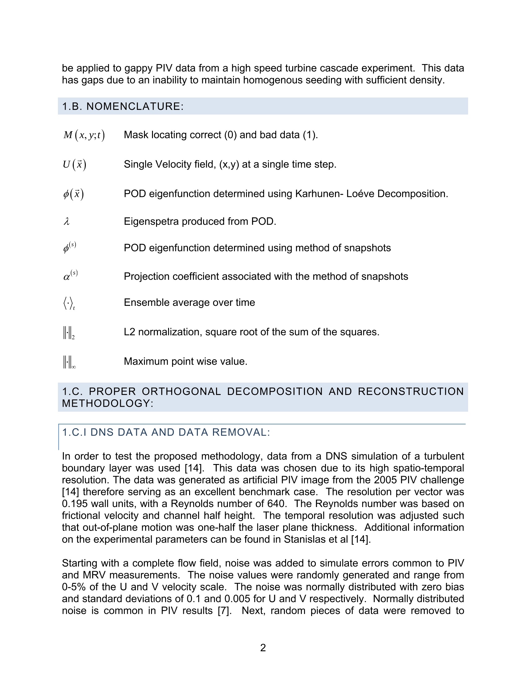
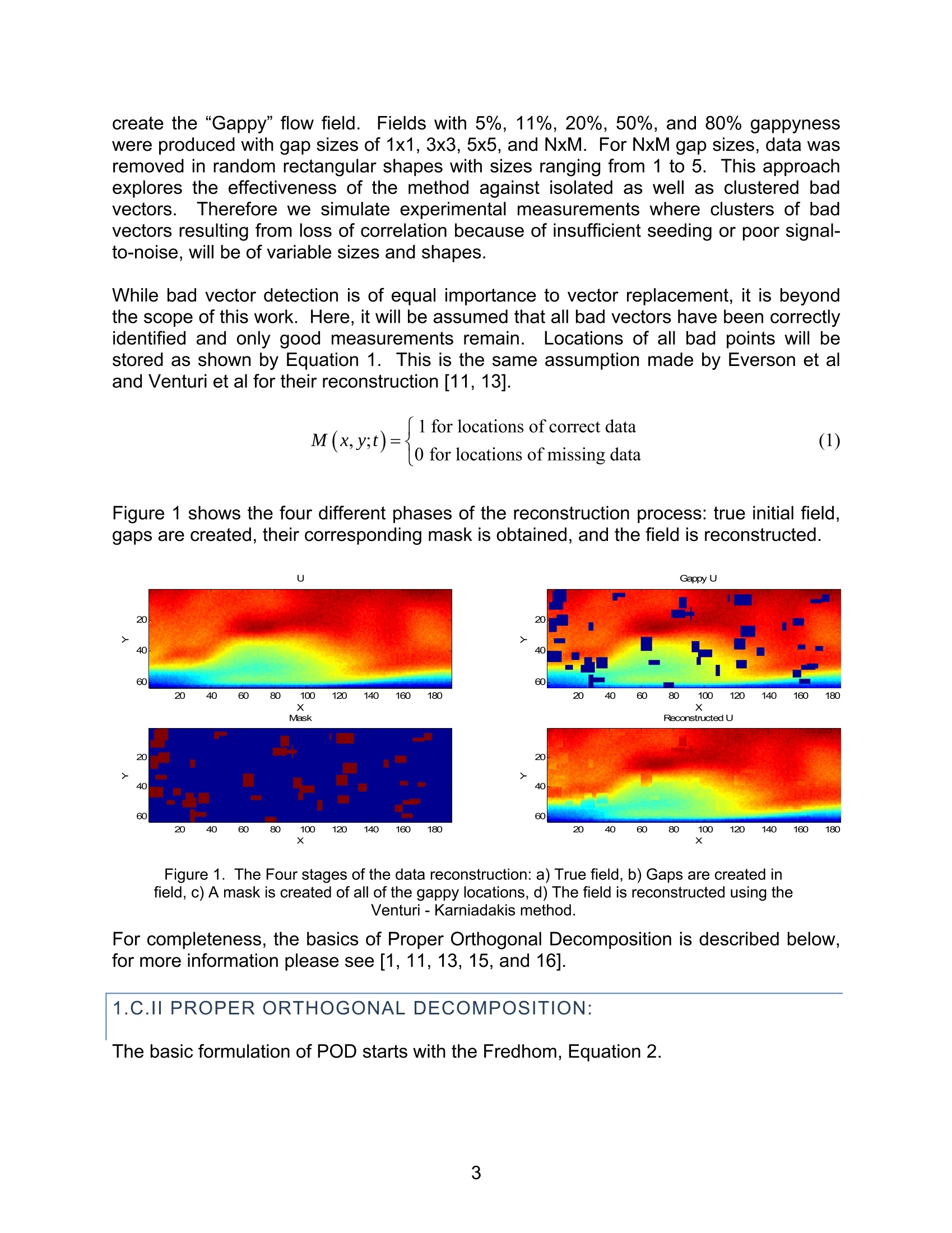
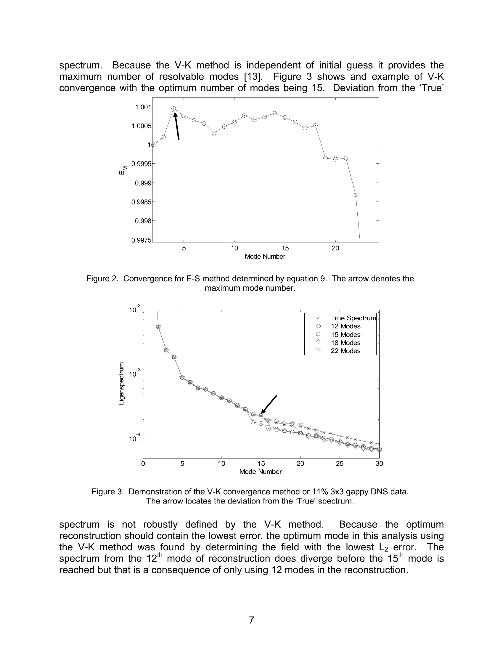

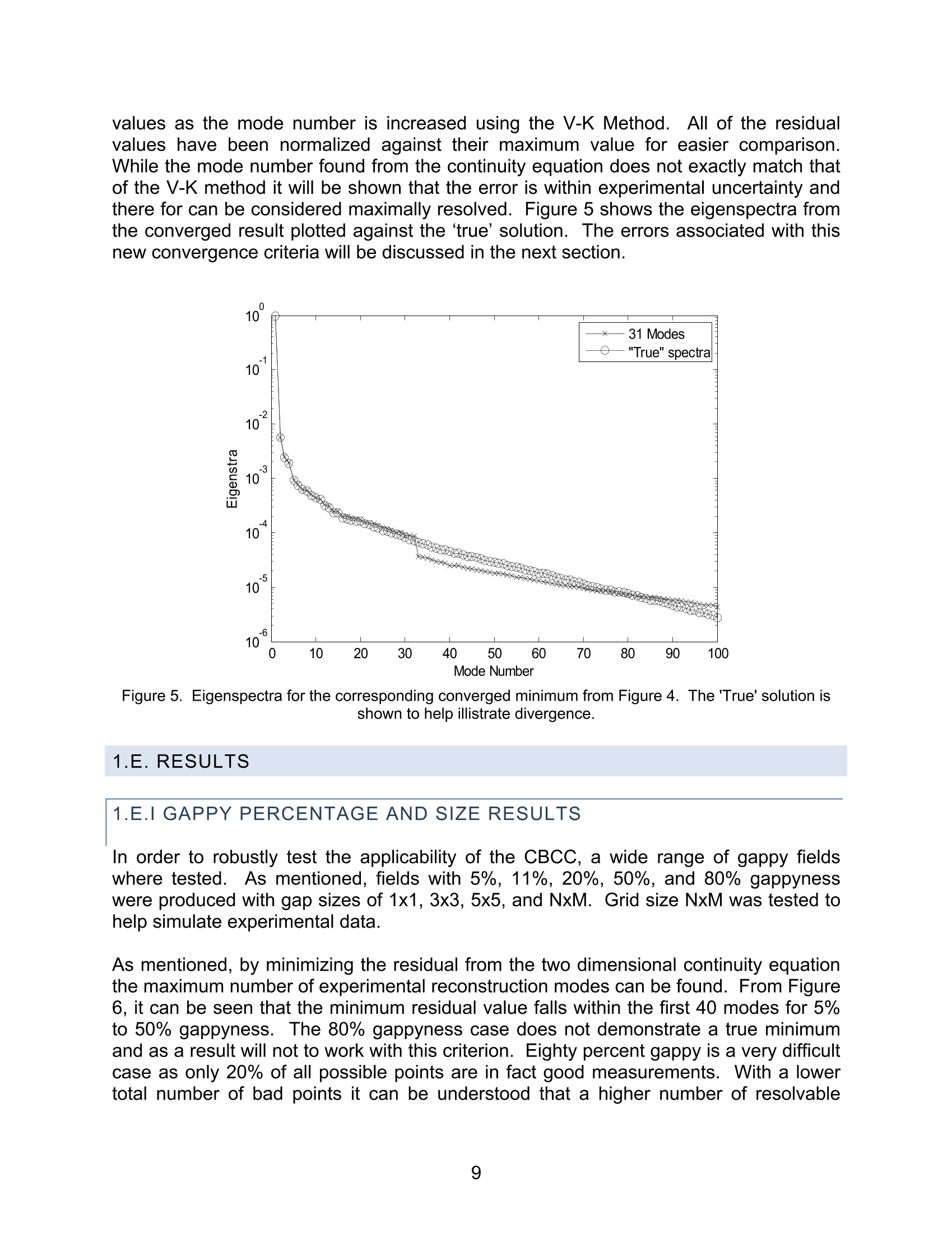
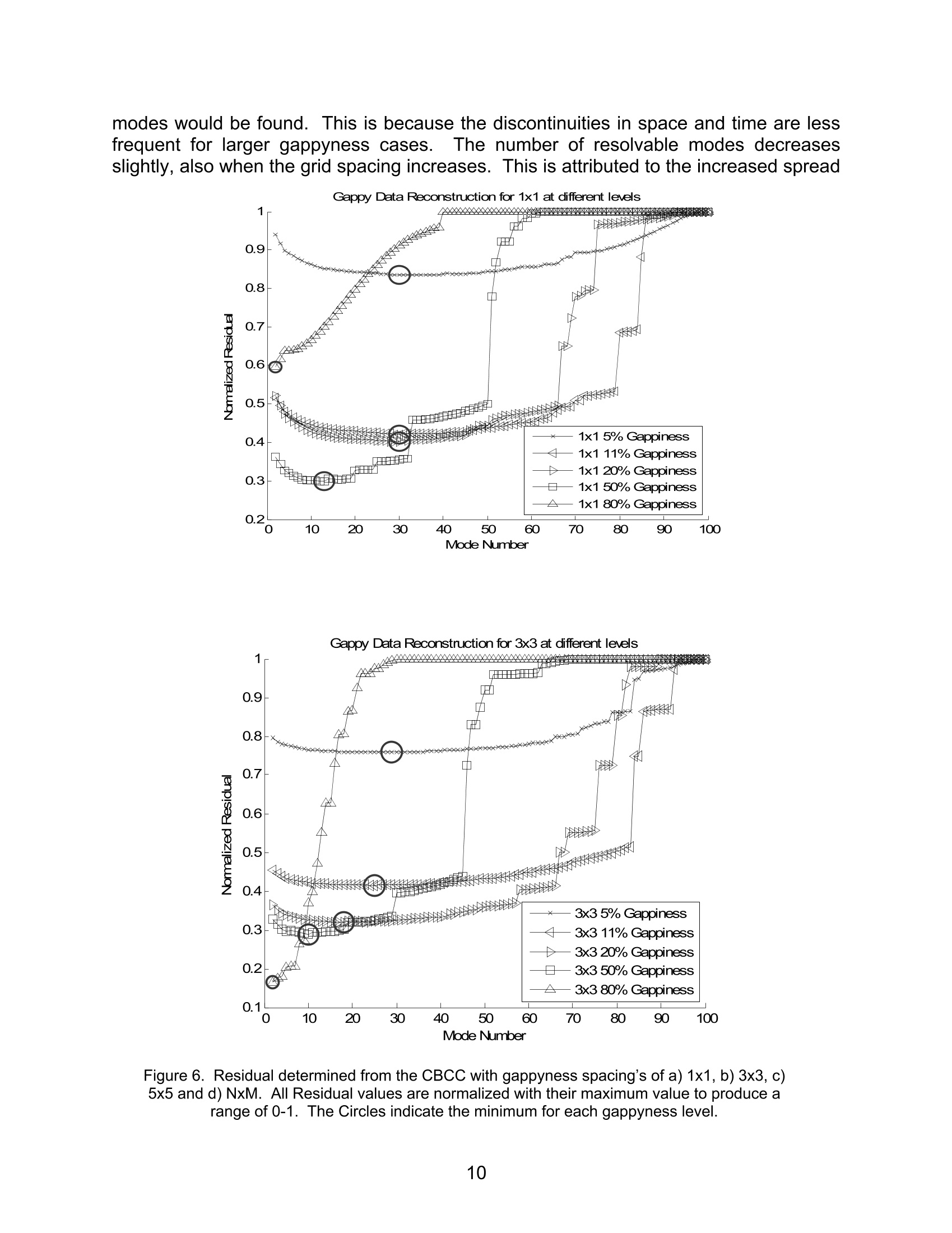
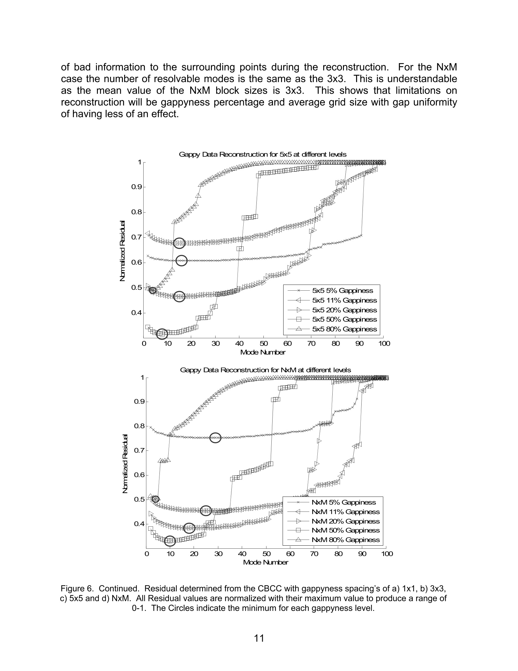
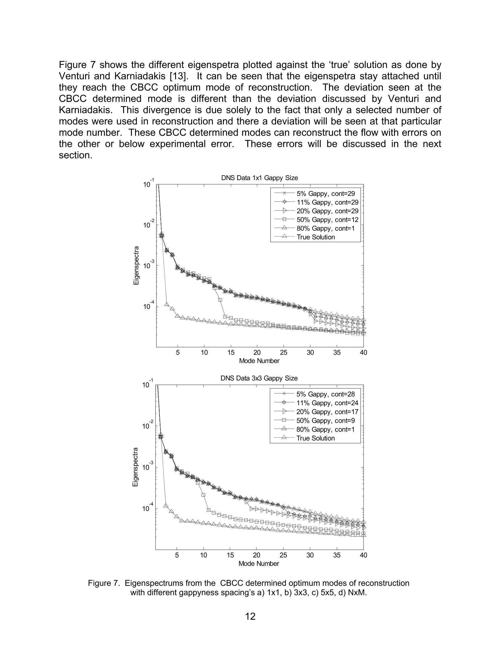
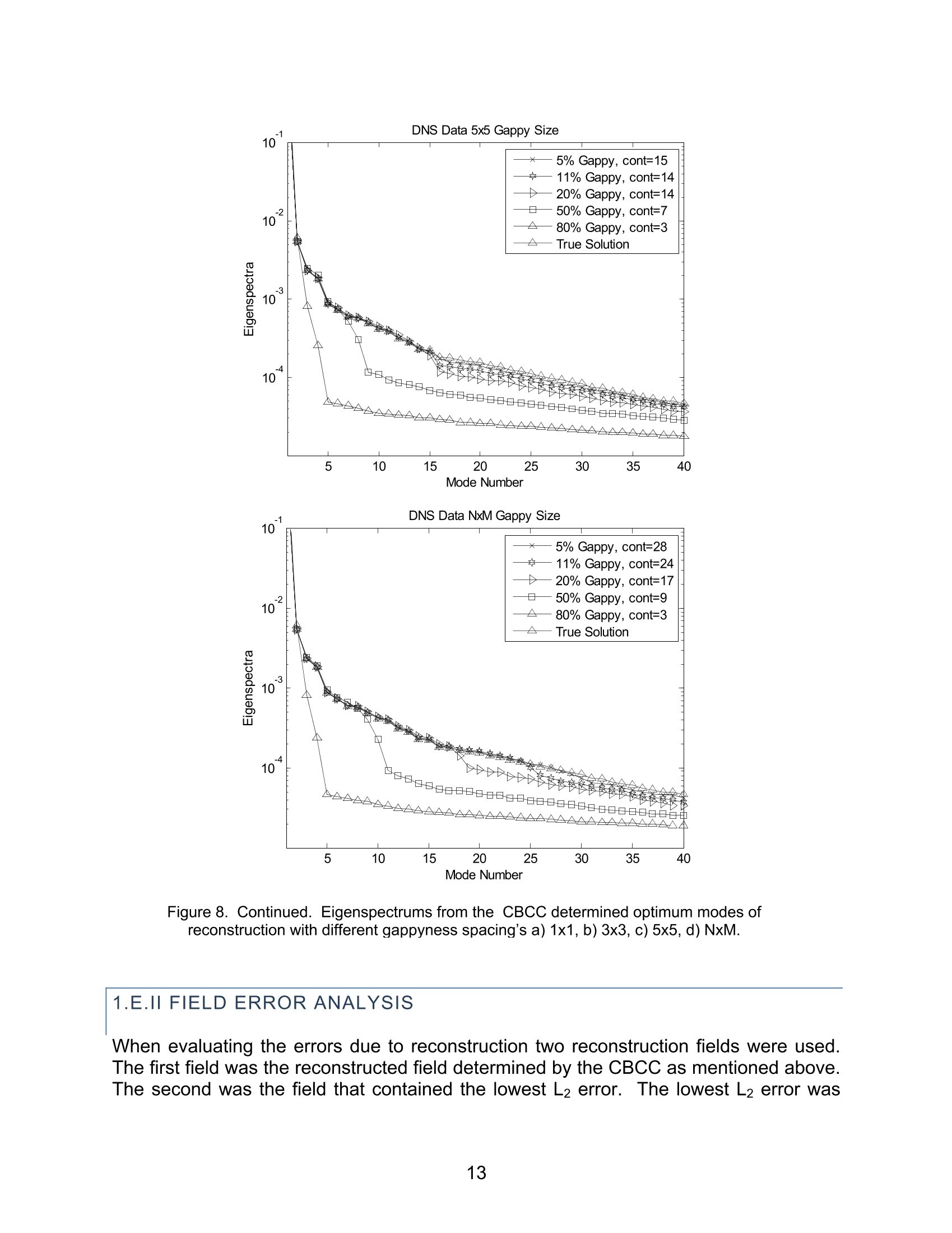
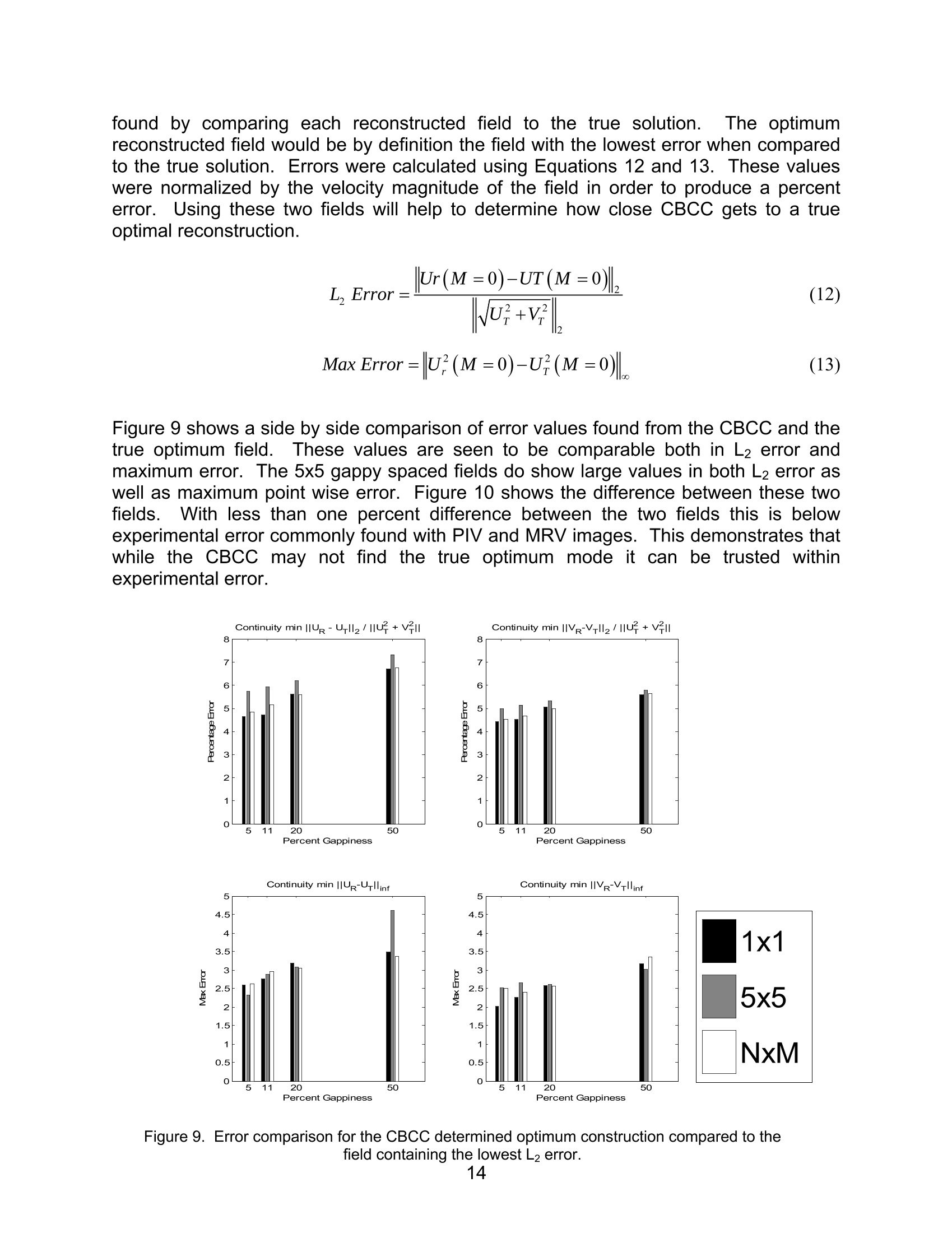

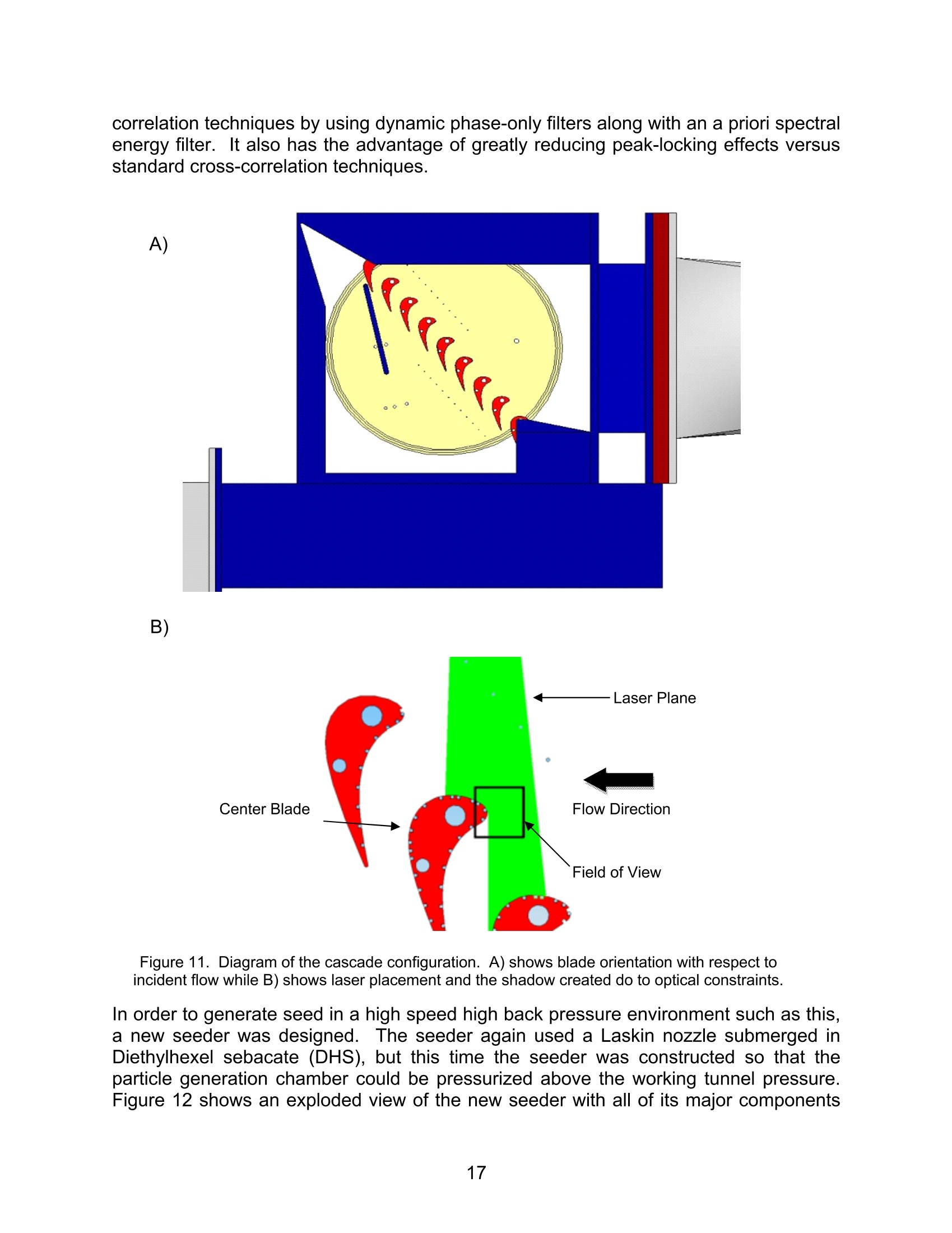
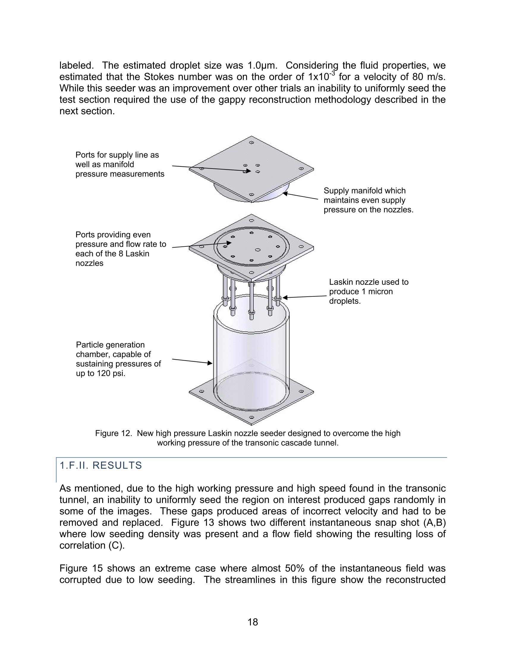
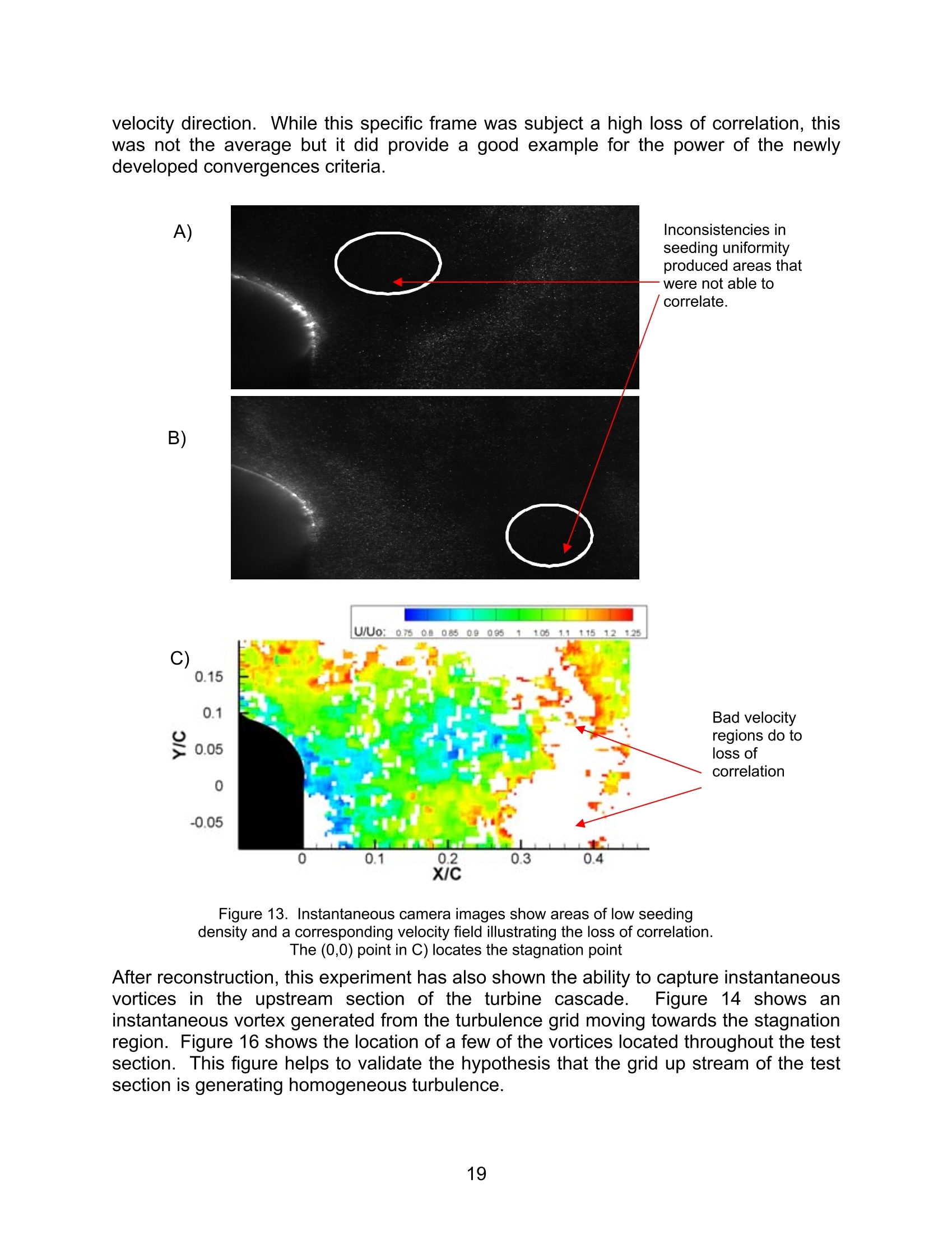
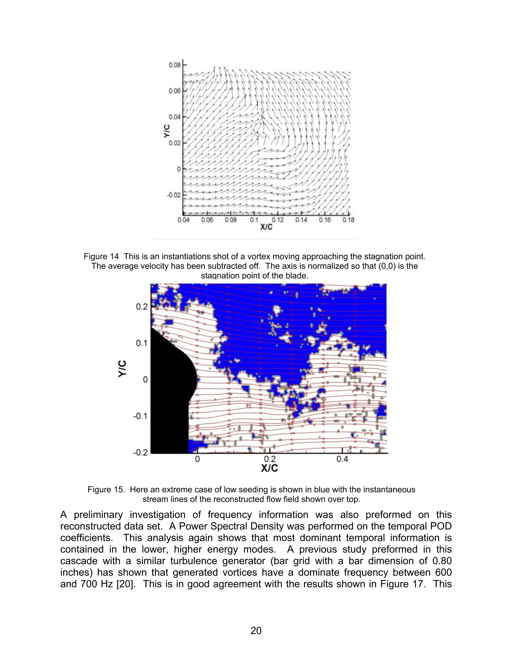
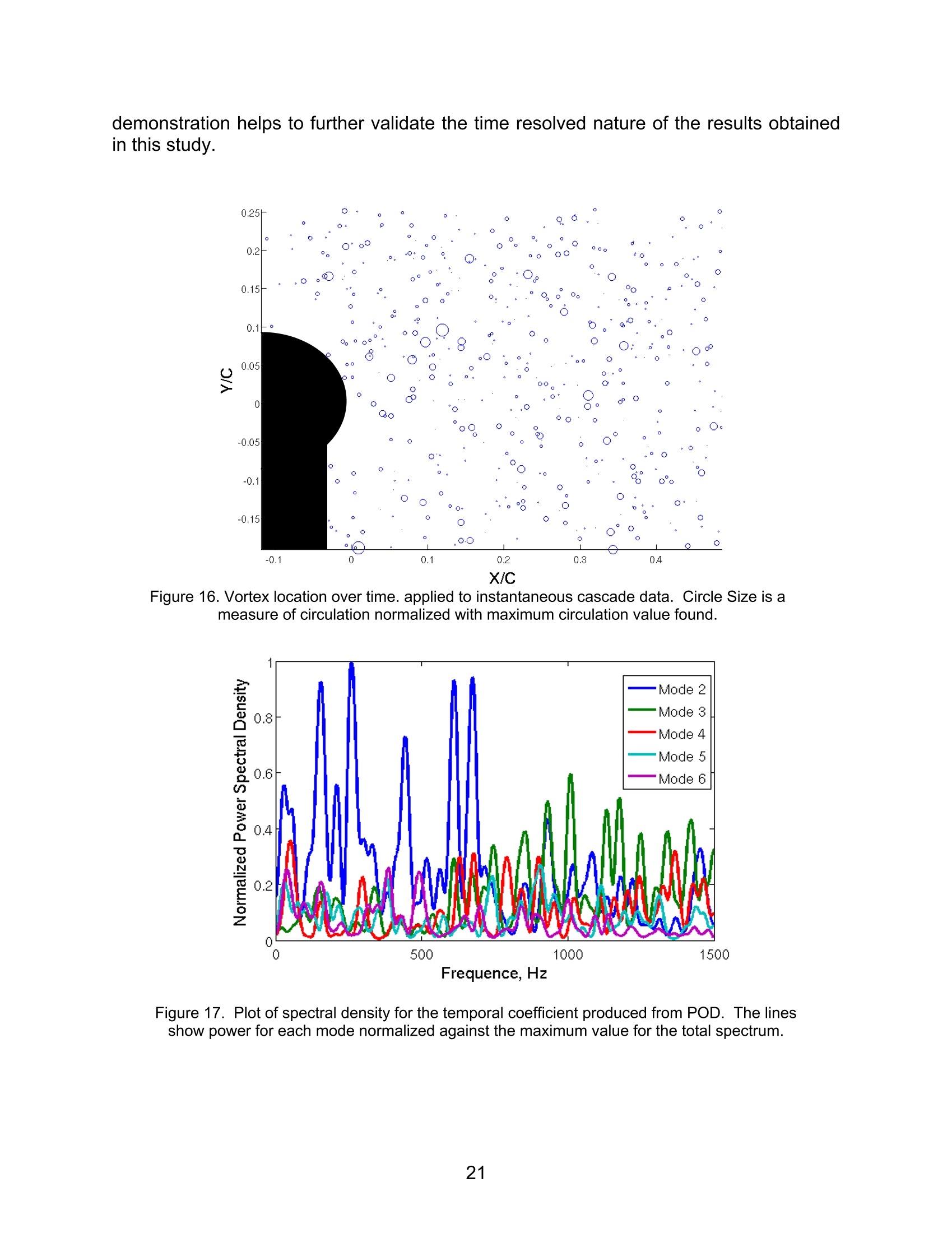

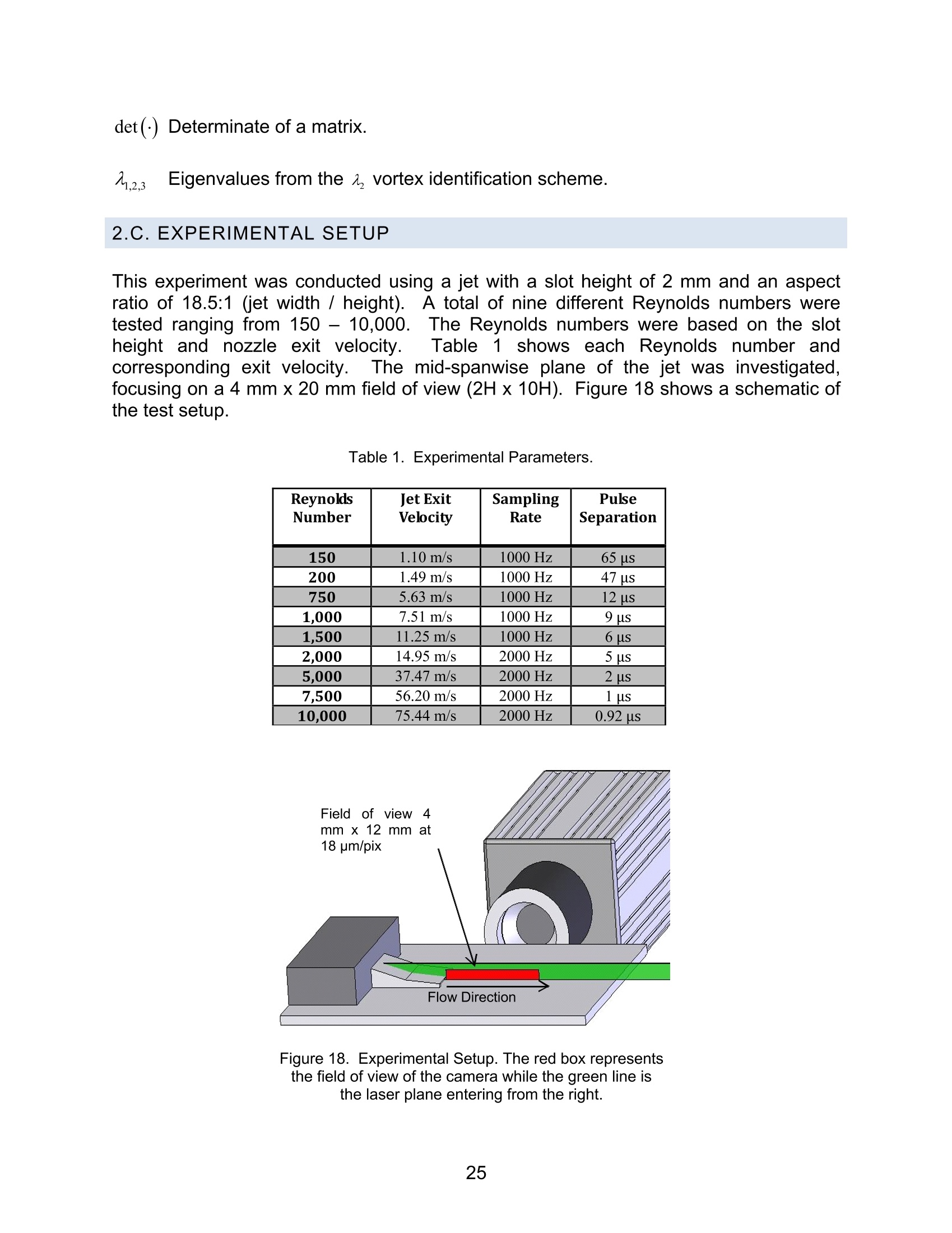
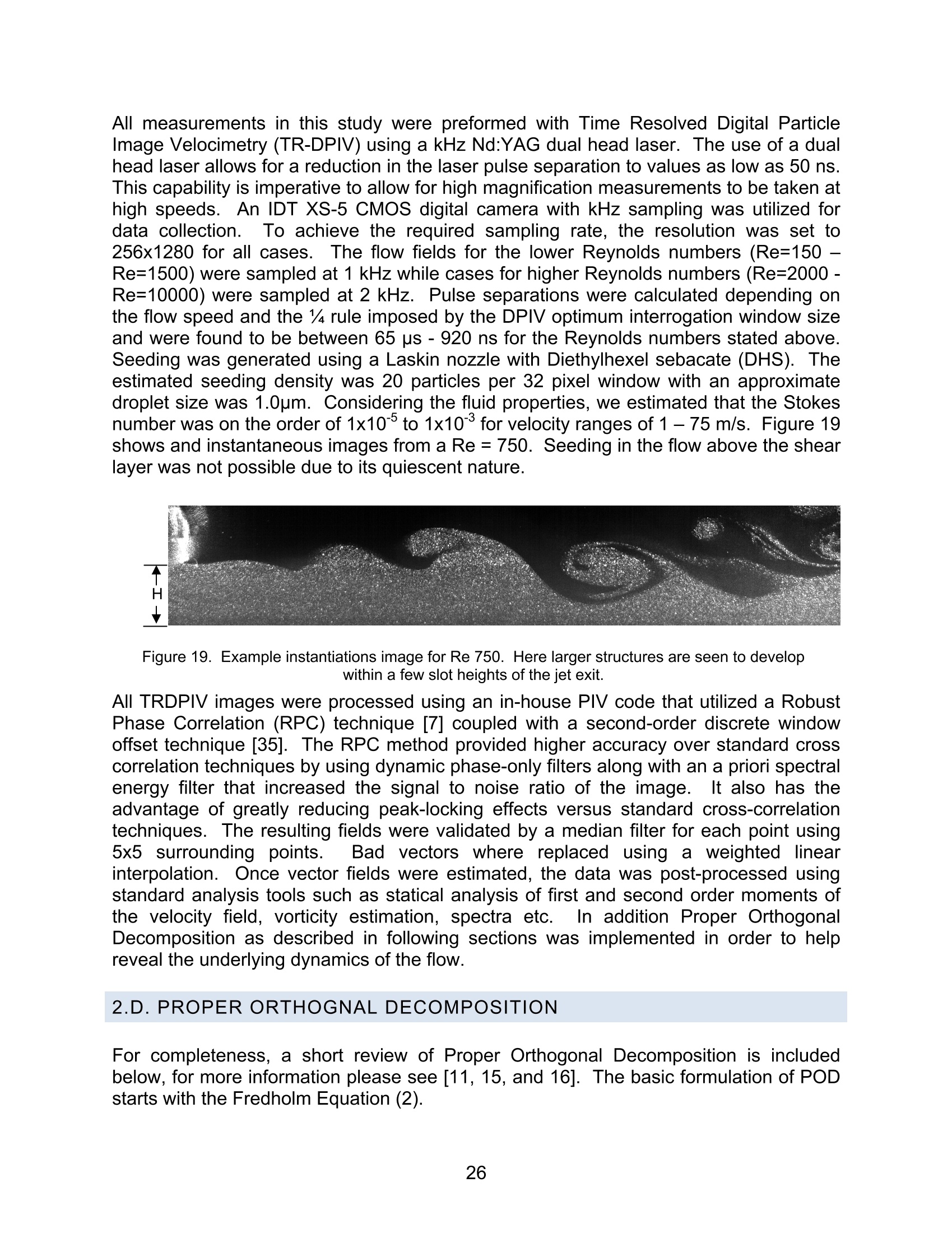
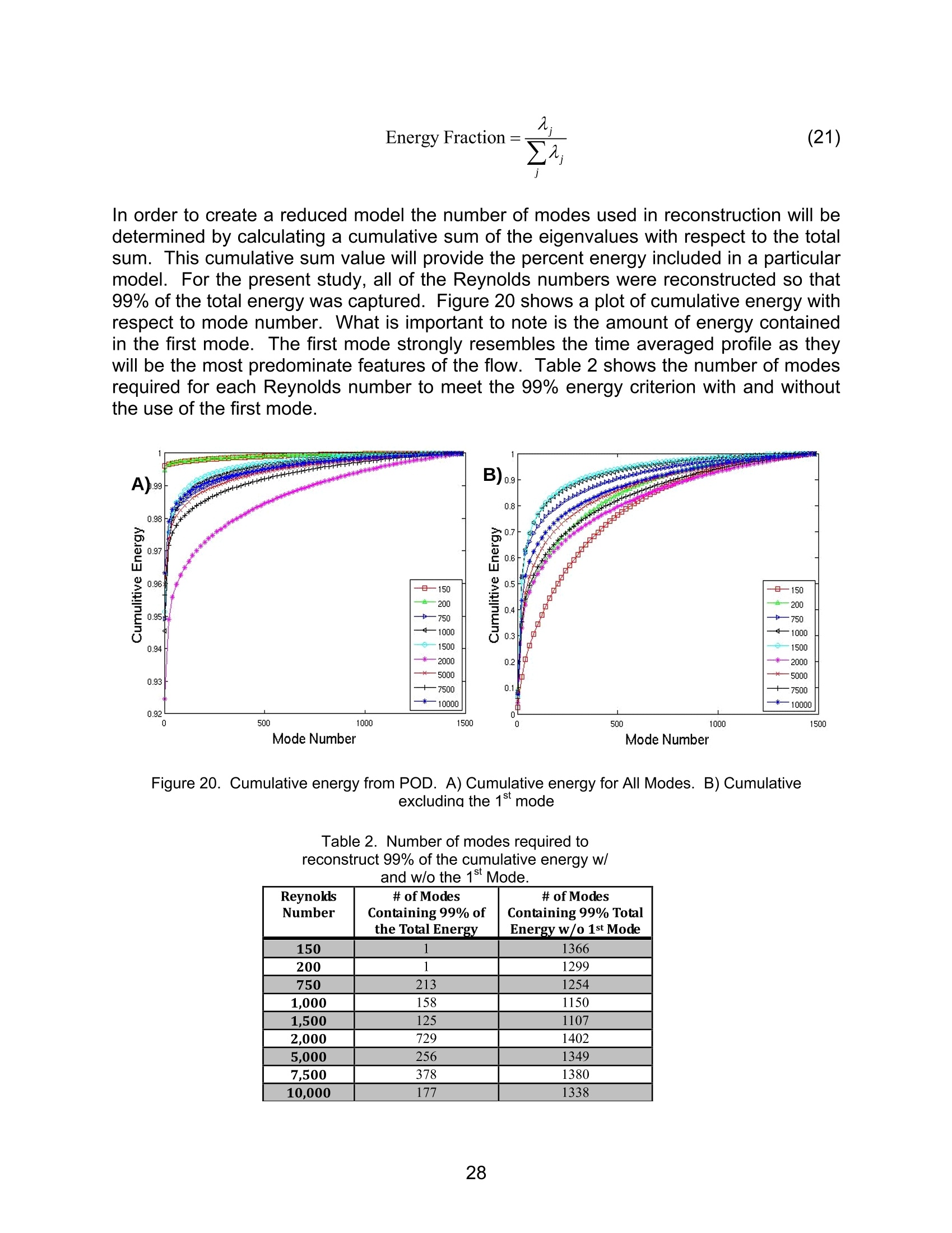
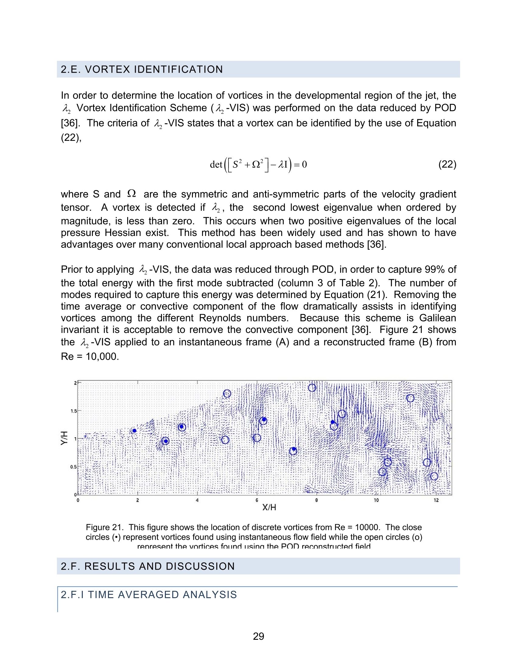
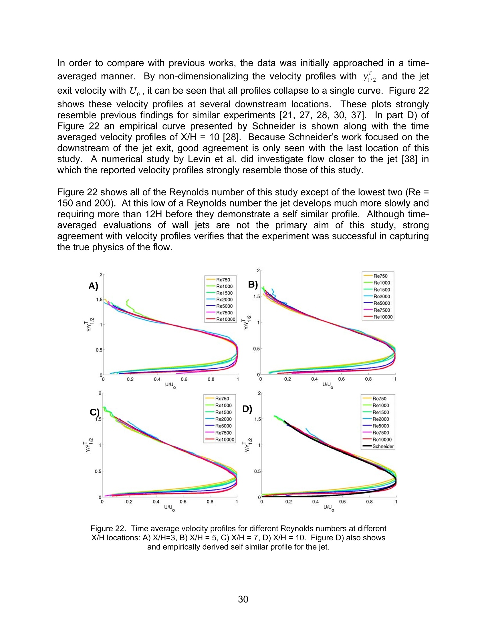
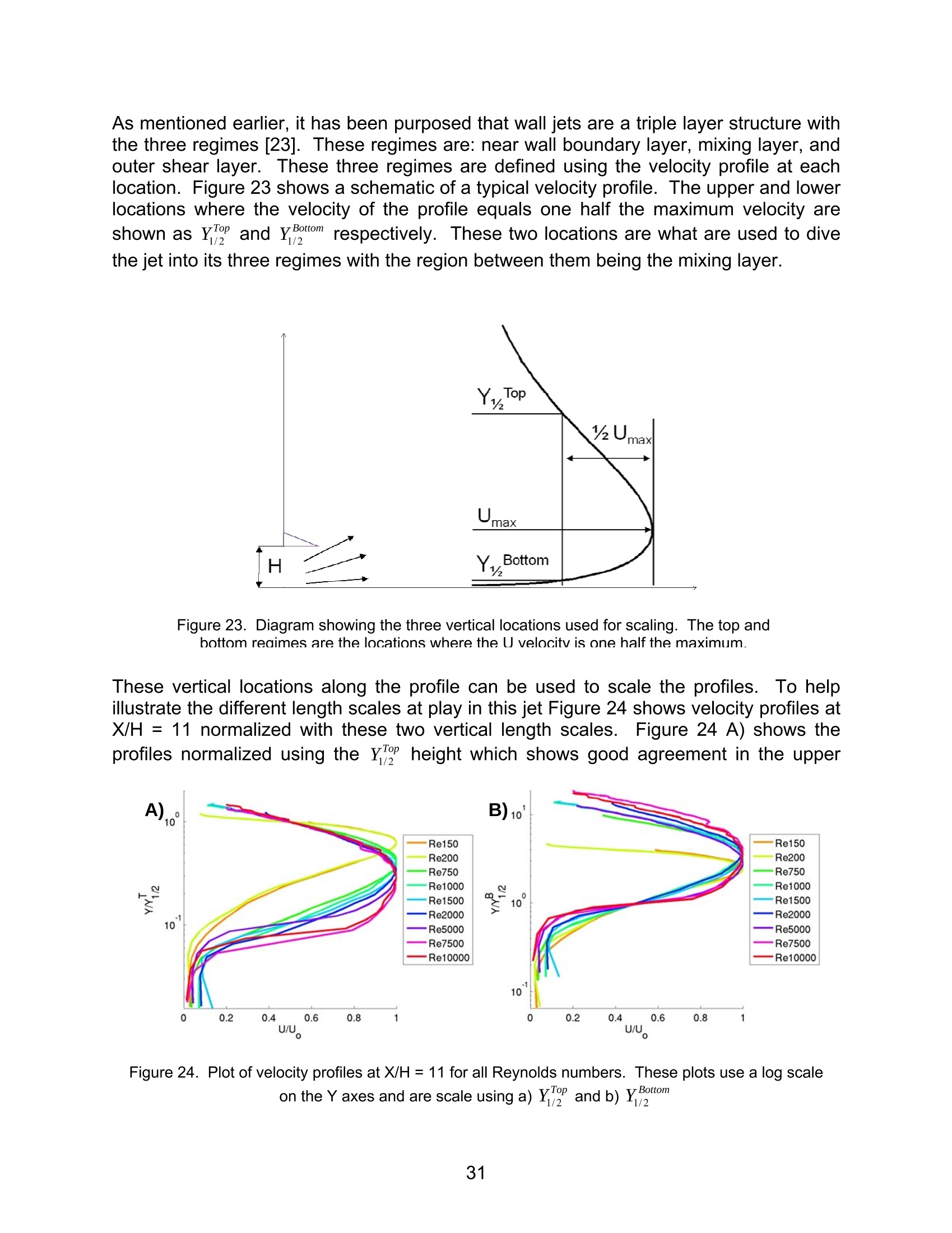

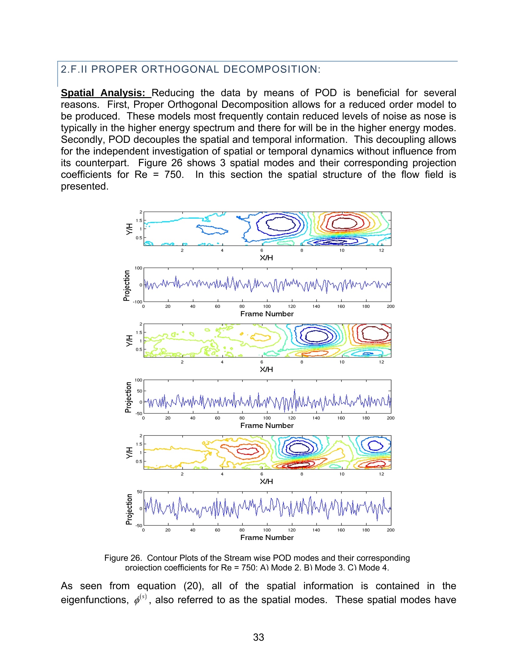
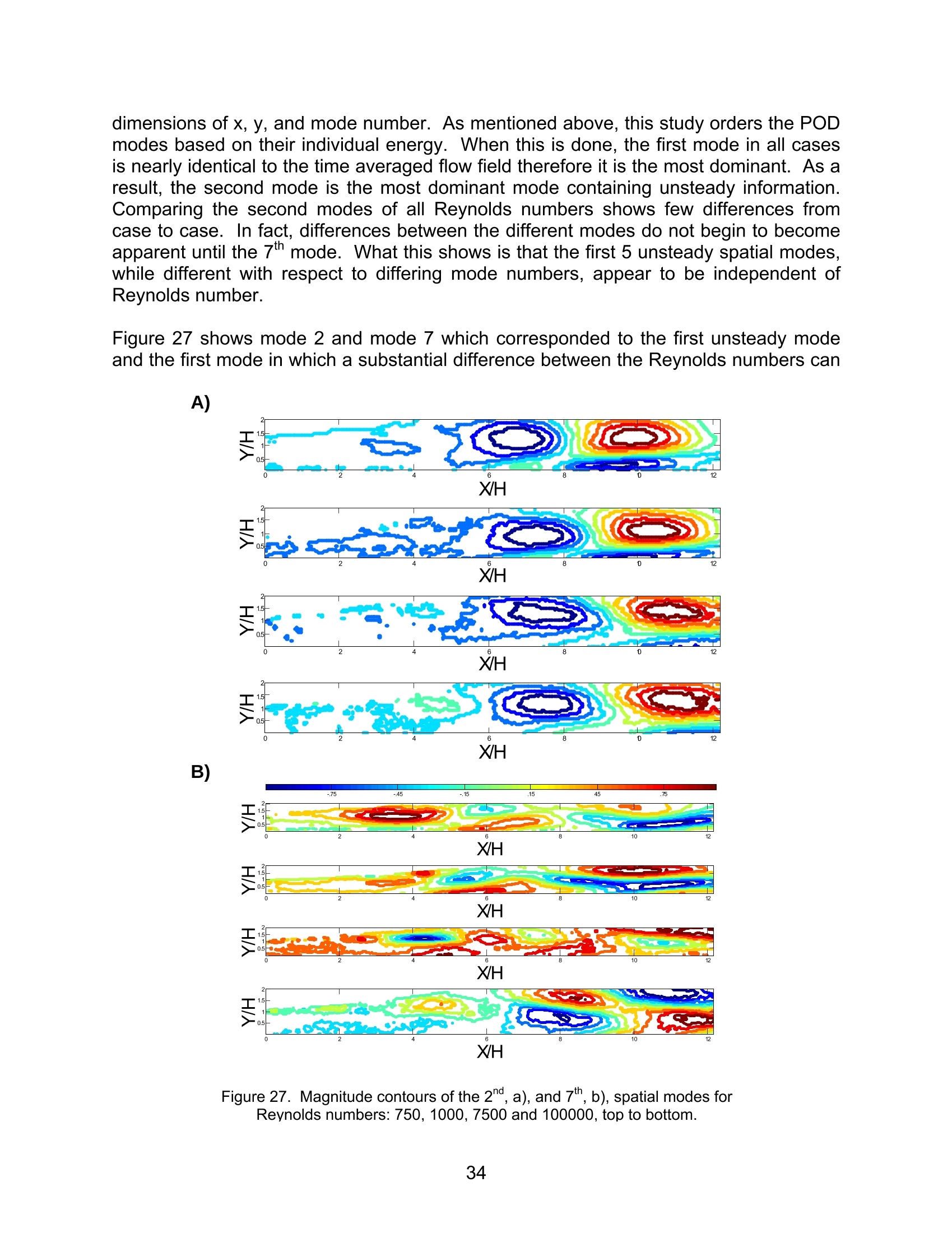
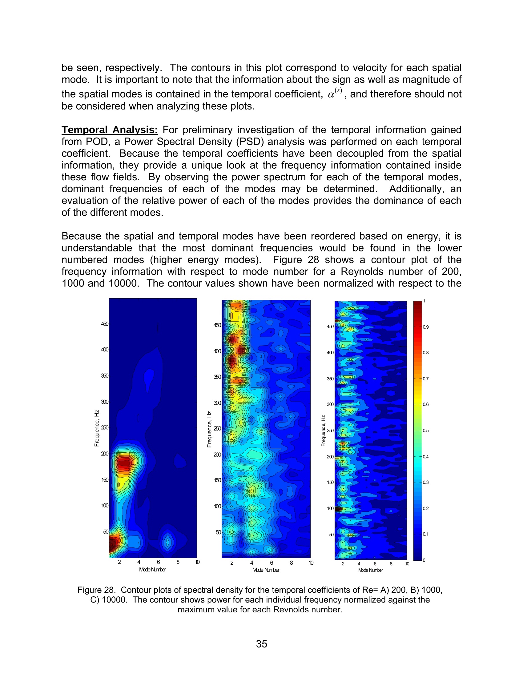
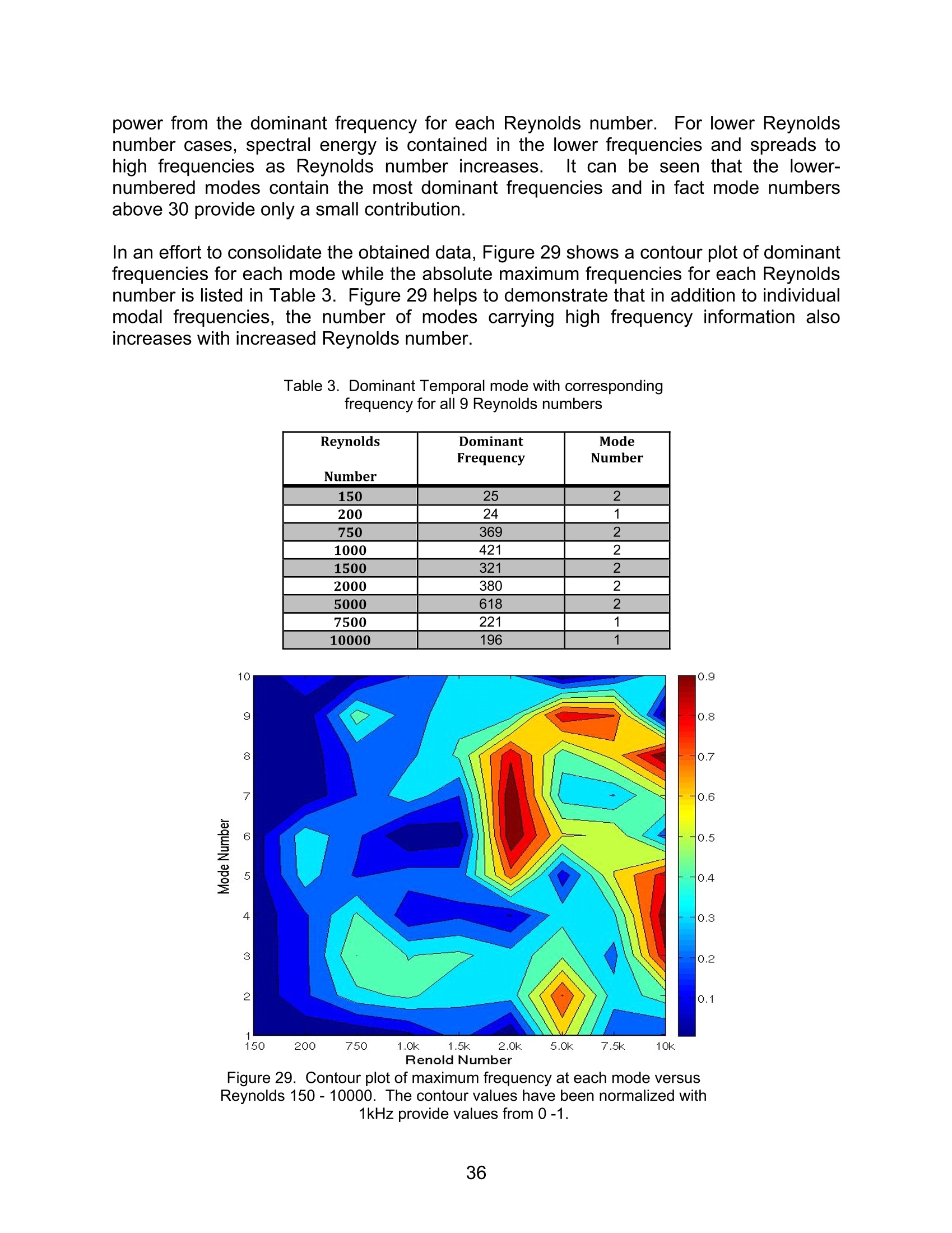
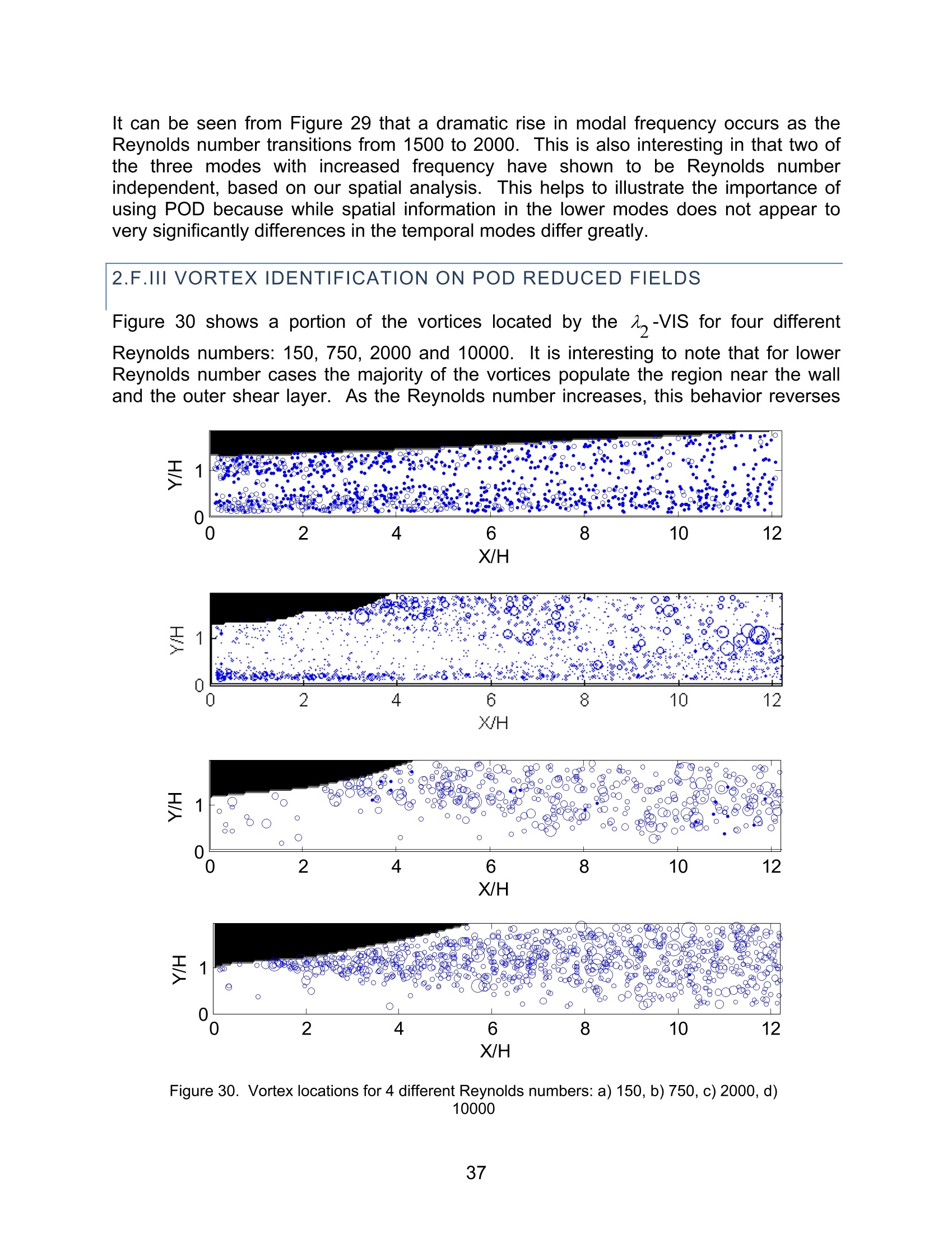
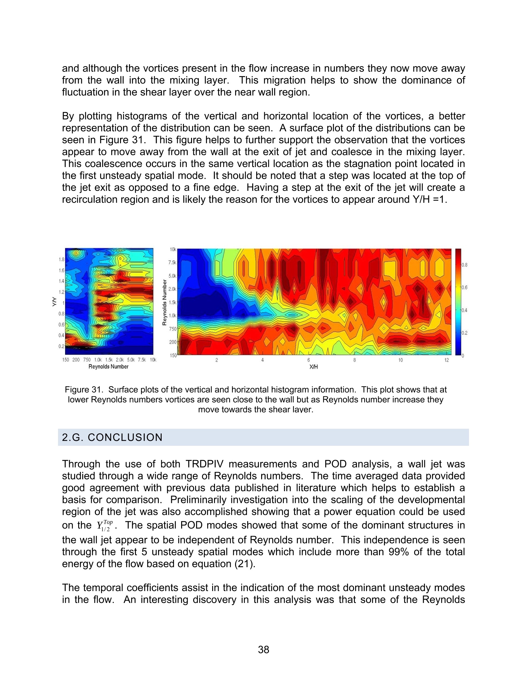


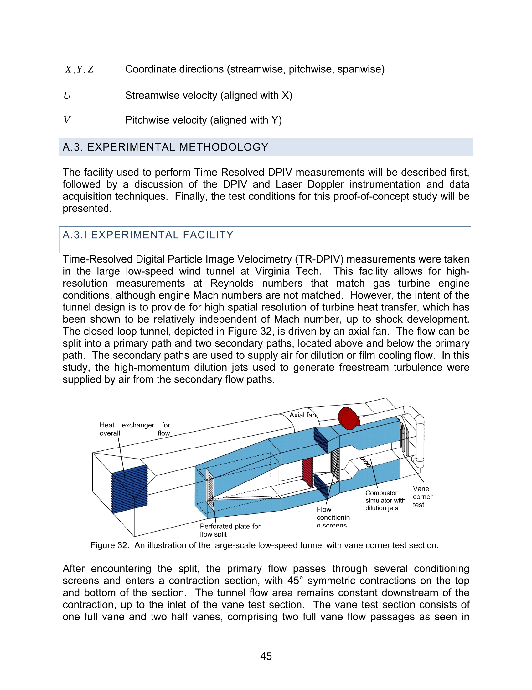
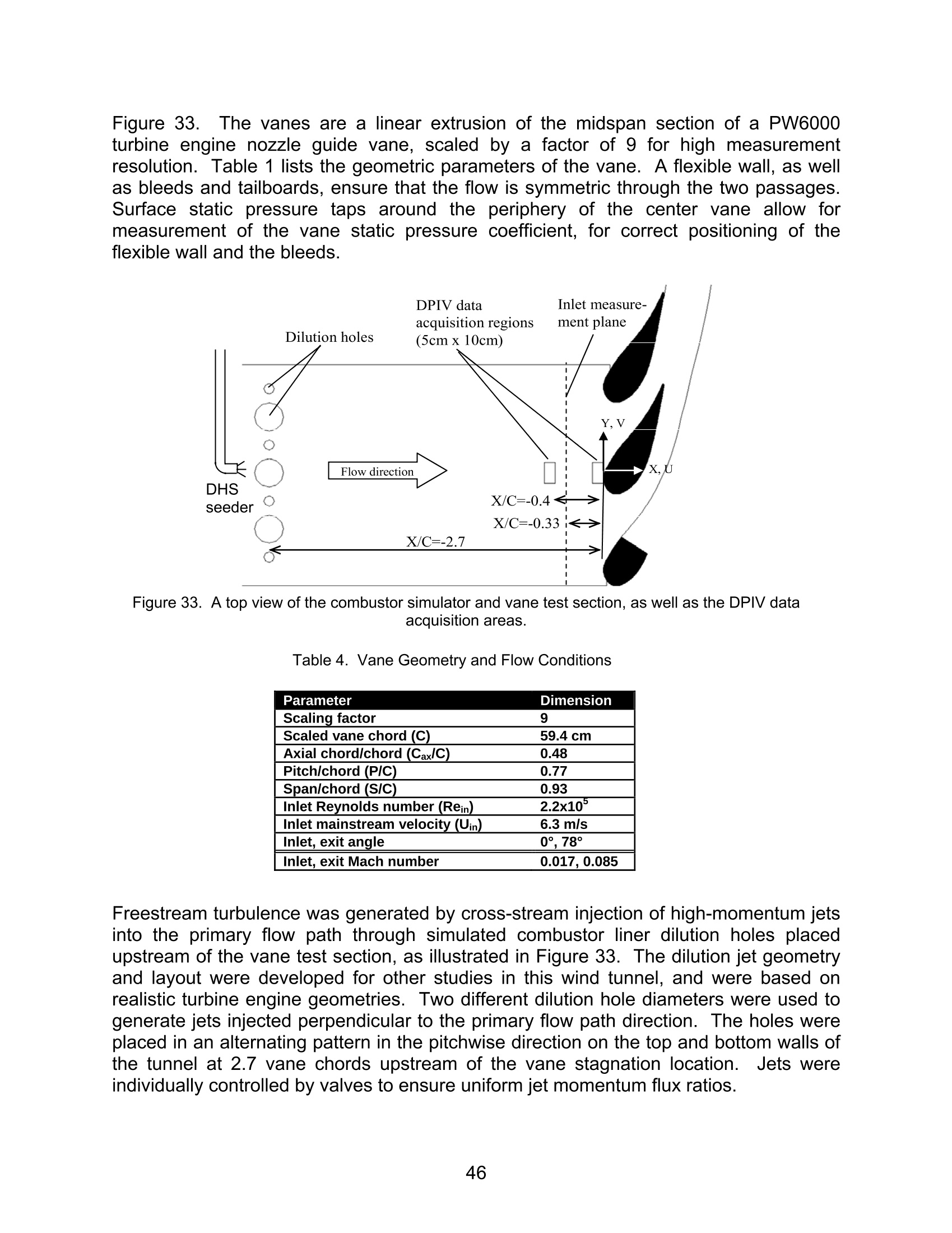
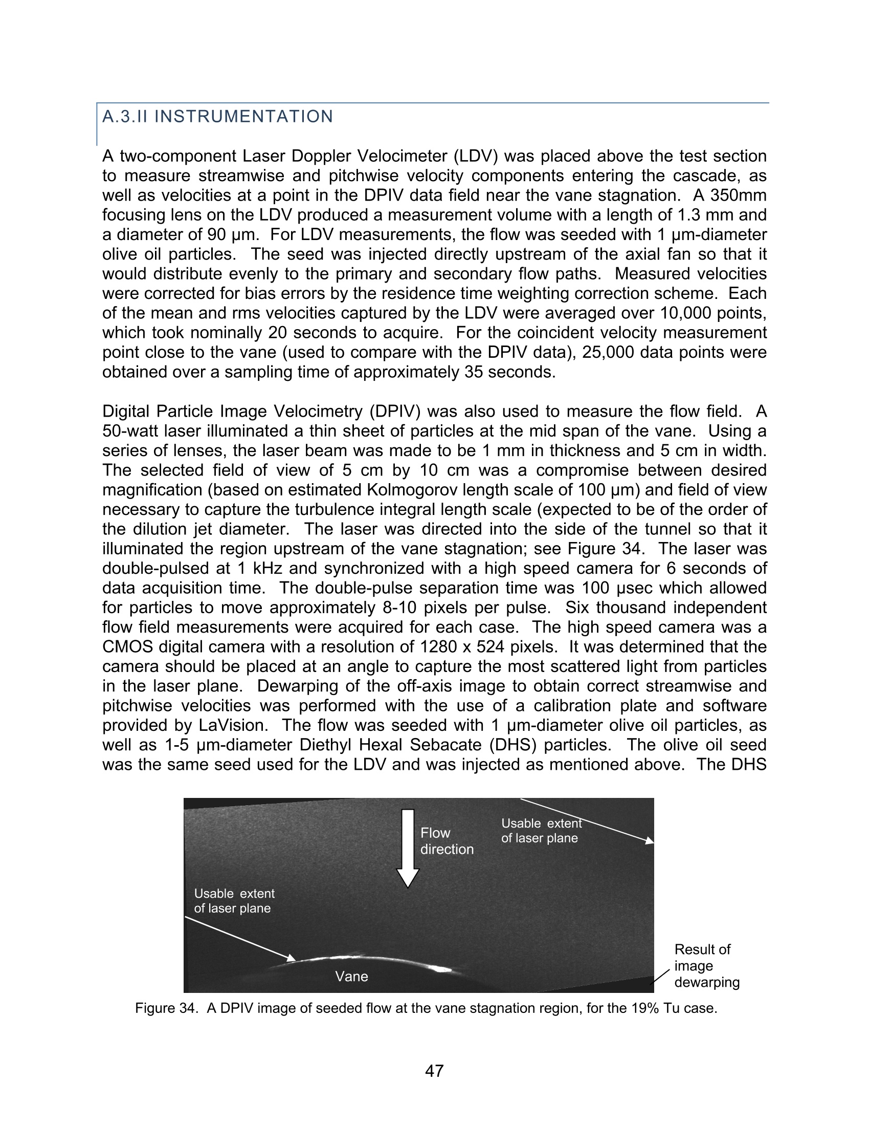
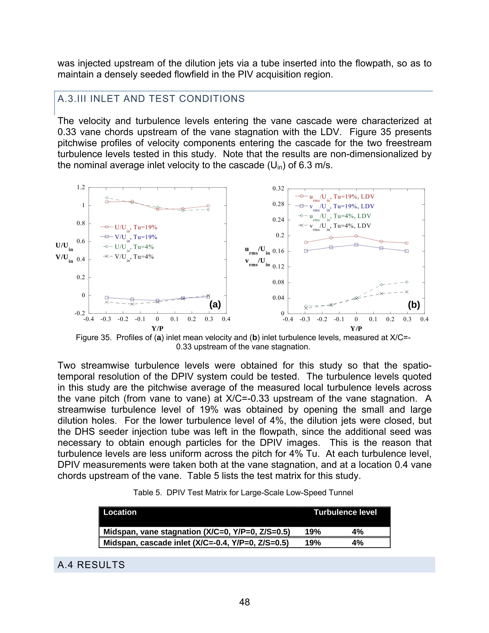
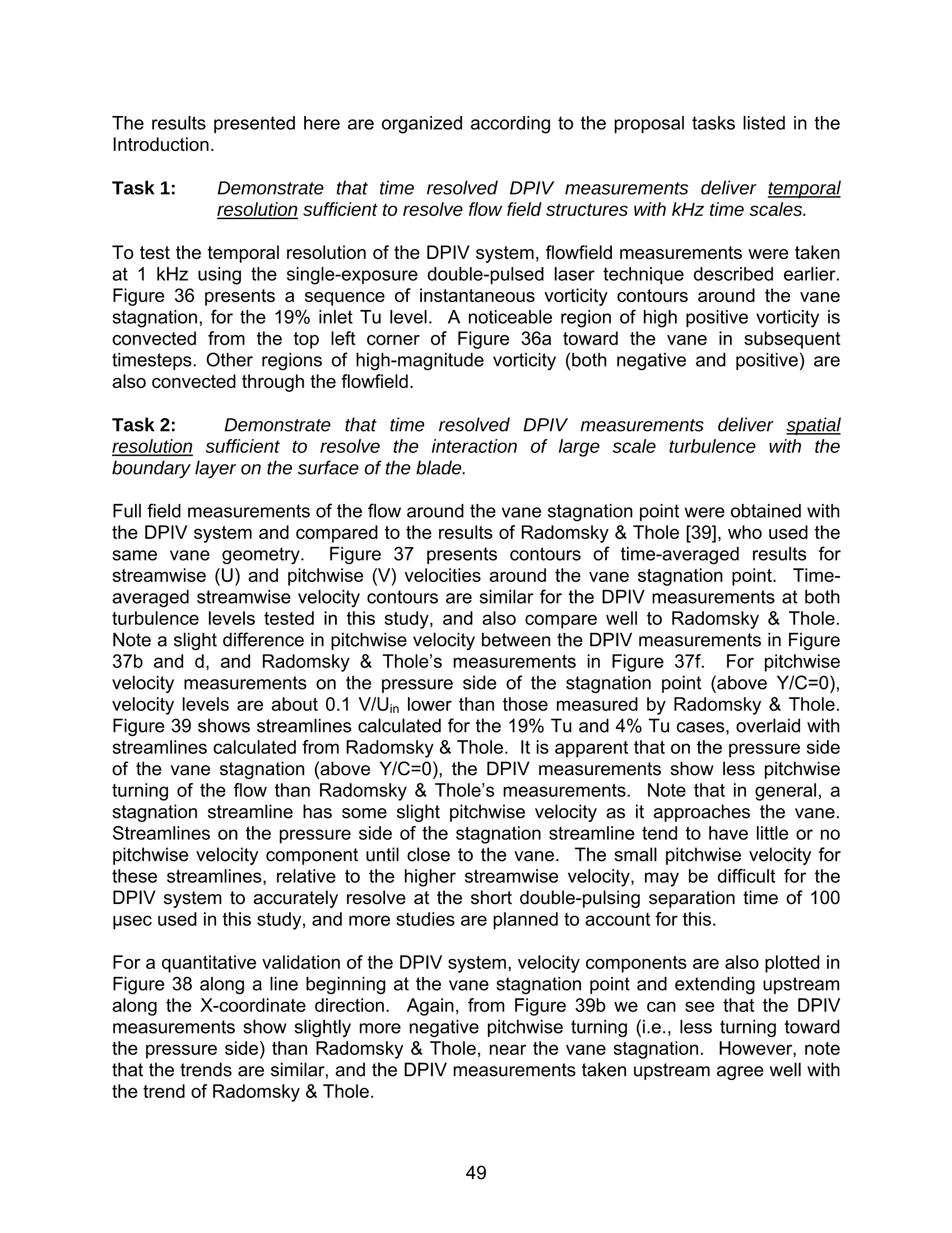

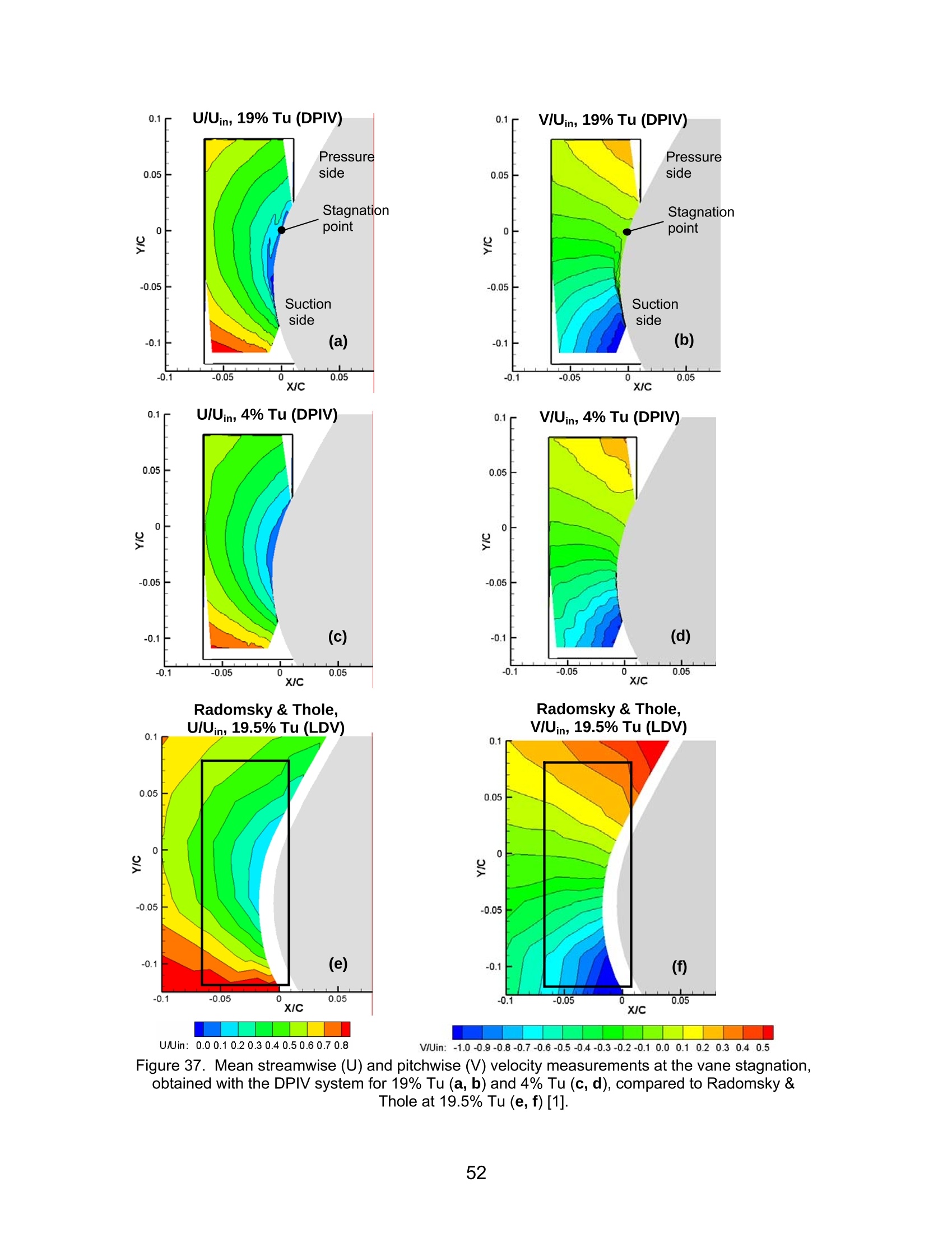
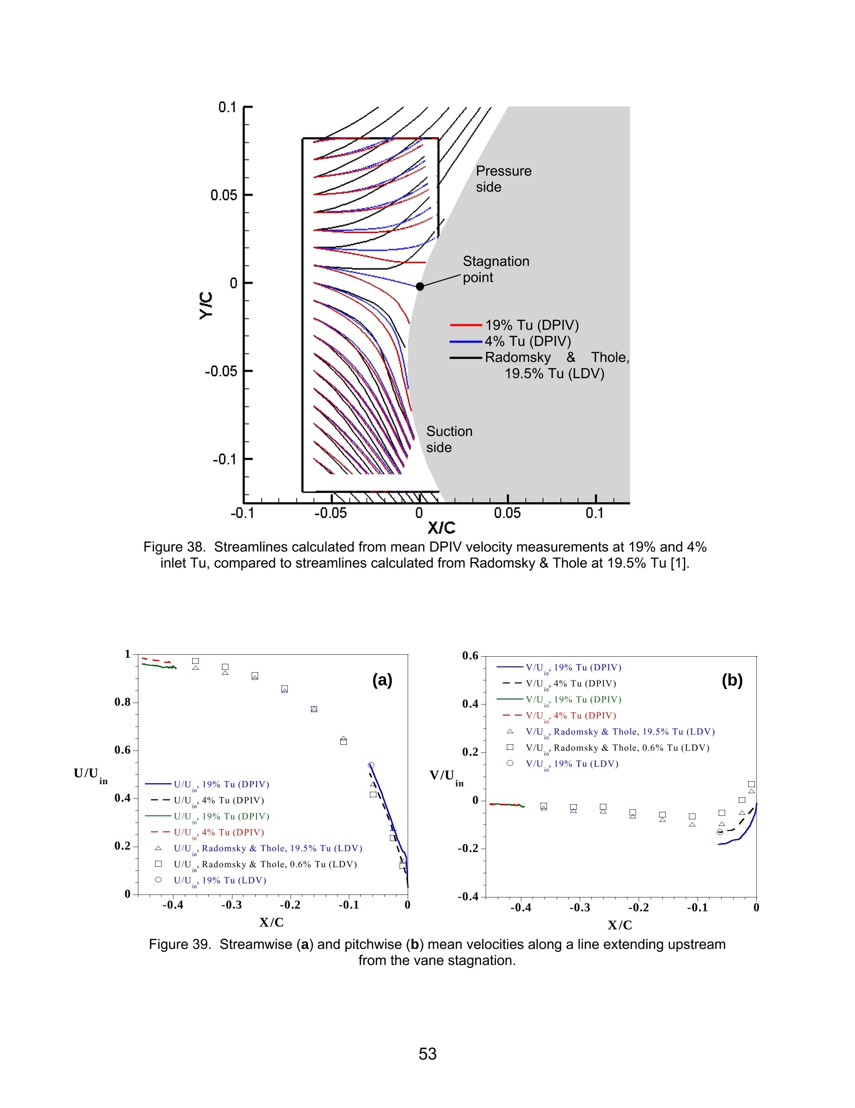
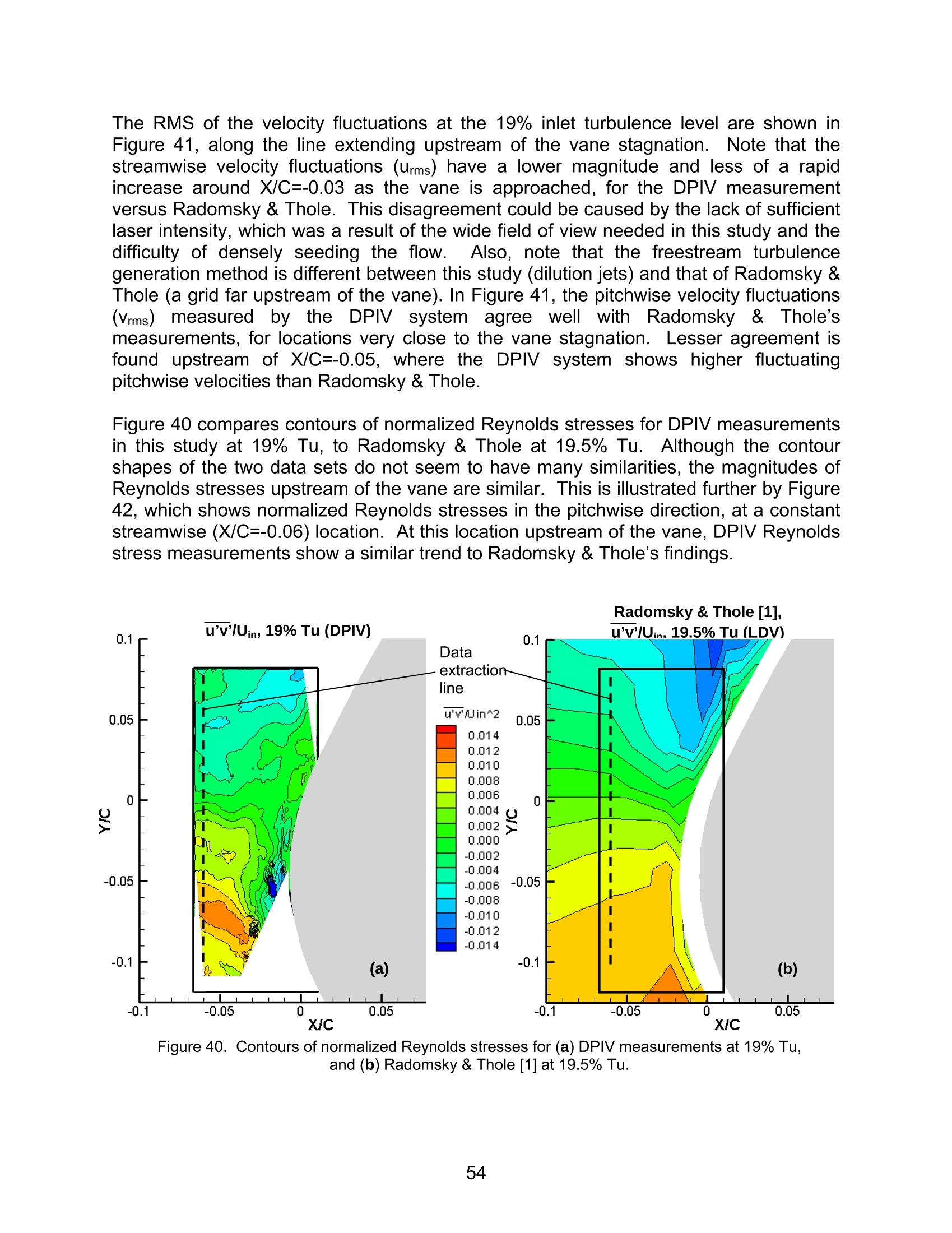
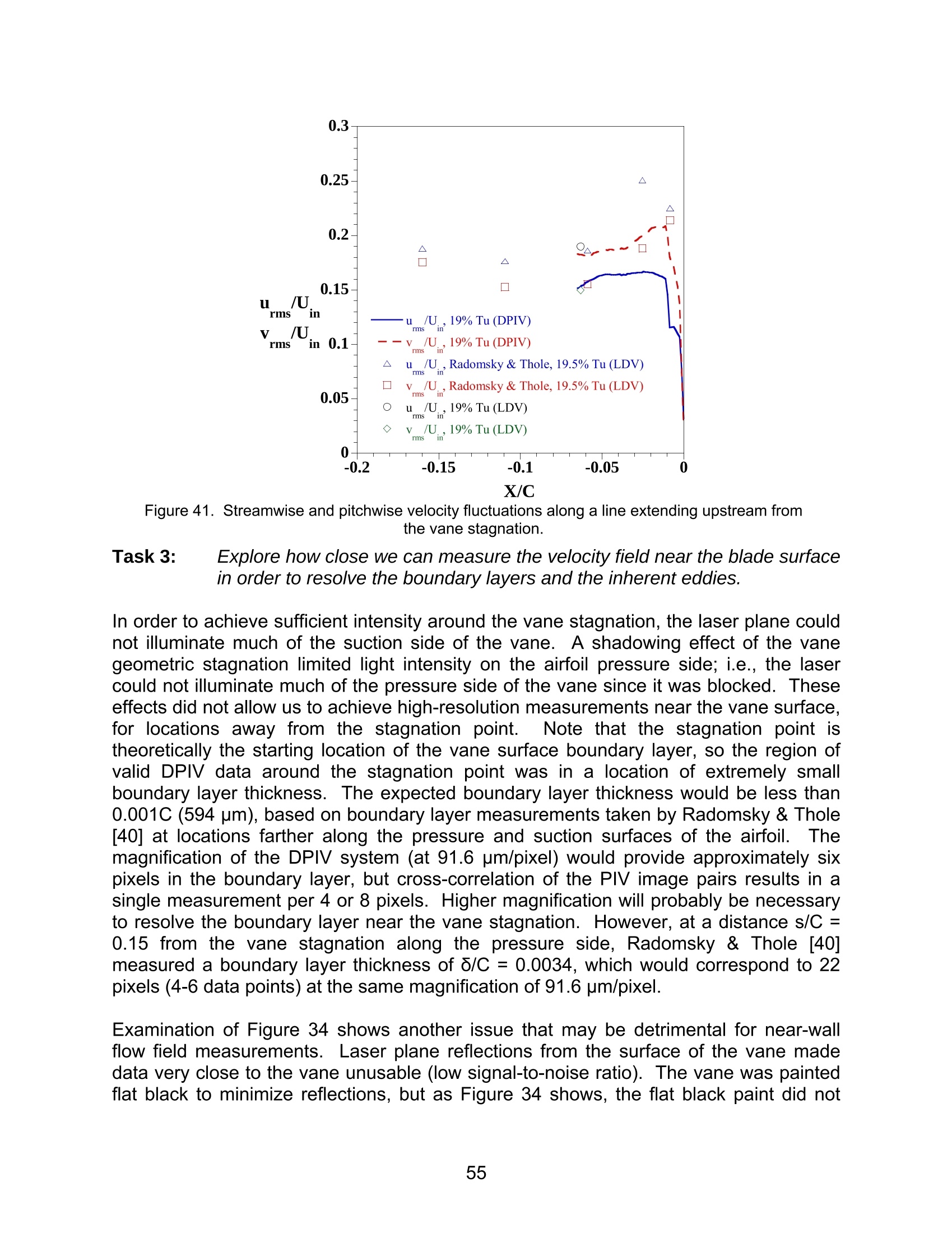

还剩64页未读,是否继续阅读?

产品配置单


北京欧兰科技发展有限公司为您提供《流体中速度场,速度矢量场检测方案(粒子图像测速)》,该方案主要用于其他中速度场,速度矢量场检测,参考标准--,《流体中速度场,速度矢量场检测方案(粒子图像测速)》用到的仪器有德国LaVision PIV/PLIF粒子成像测速场仪、Imager LX PIV相机
推荐专场


相关方案
更多
该厂商其他方案
更多