


方案详情
文
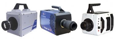
采用两组每组8台相机(LaVision Imager Pro
HS) 构成一套组合的3D3C体视抖盒子测量系统。每组相机系统可以获得90 × 60 × 25 cm3大小的体视流场,两套系统测量对象空间有30cm重叠,最终实现150 × 60 × 25 cm3尺度的流场测量结果。并将之应用于湍流边界层。
方案详情

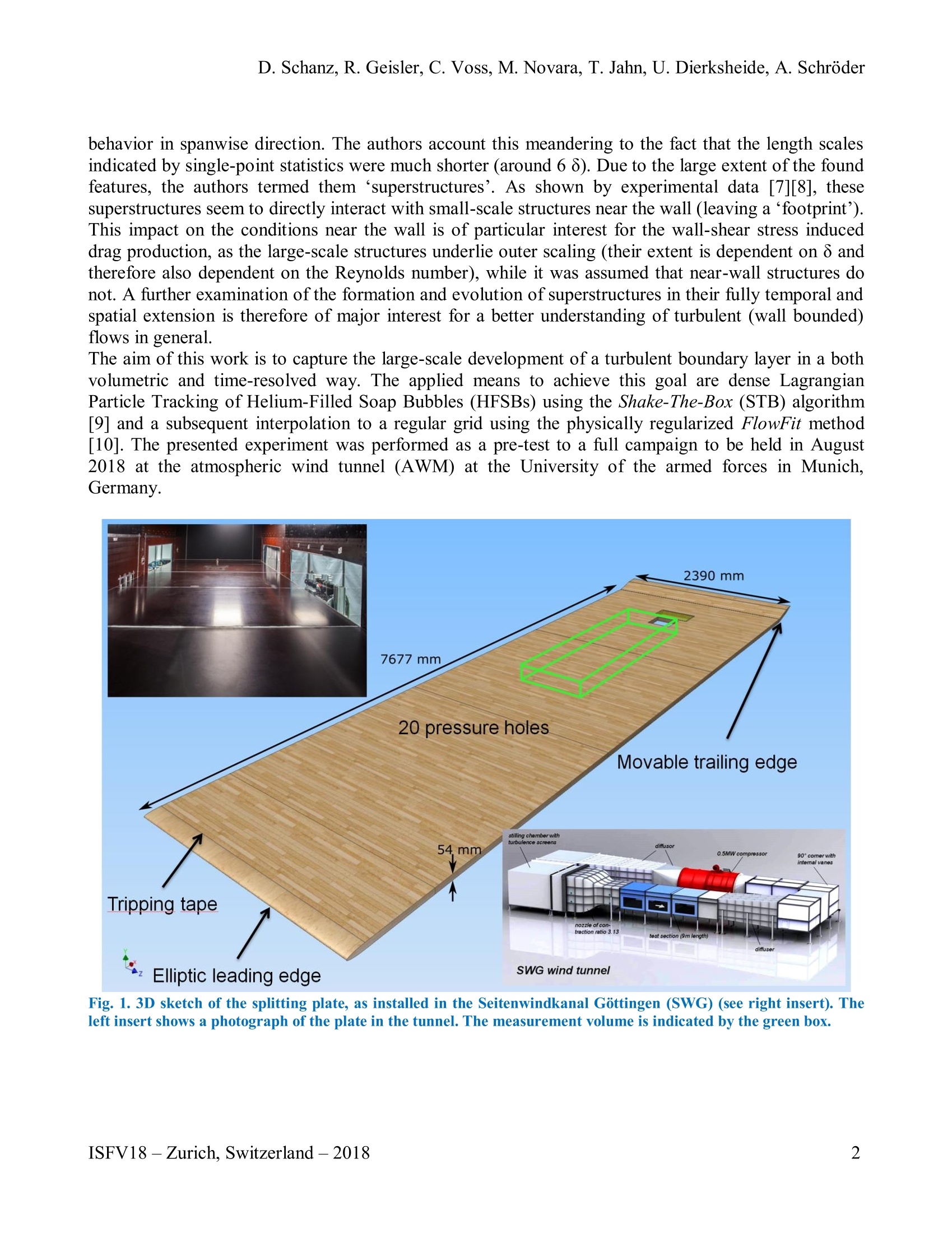
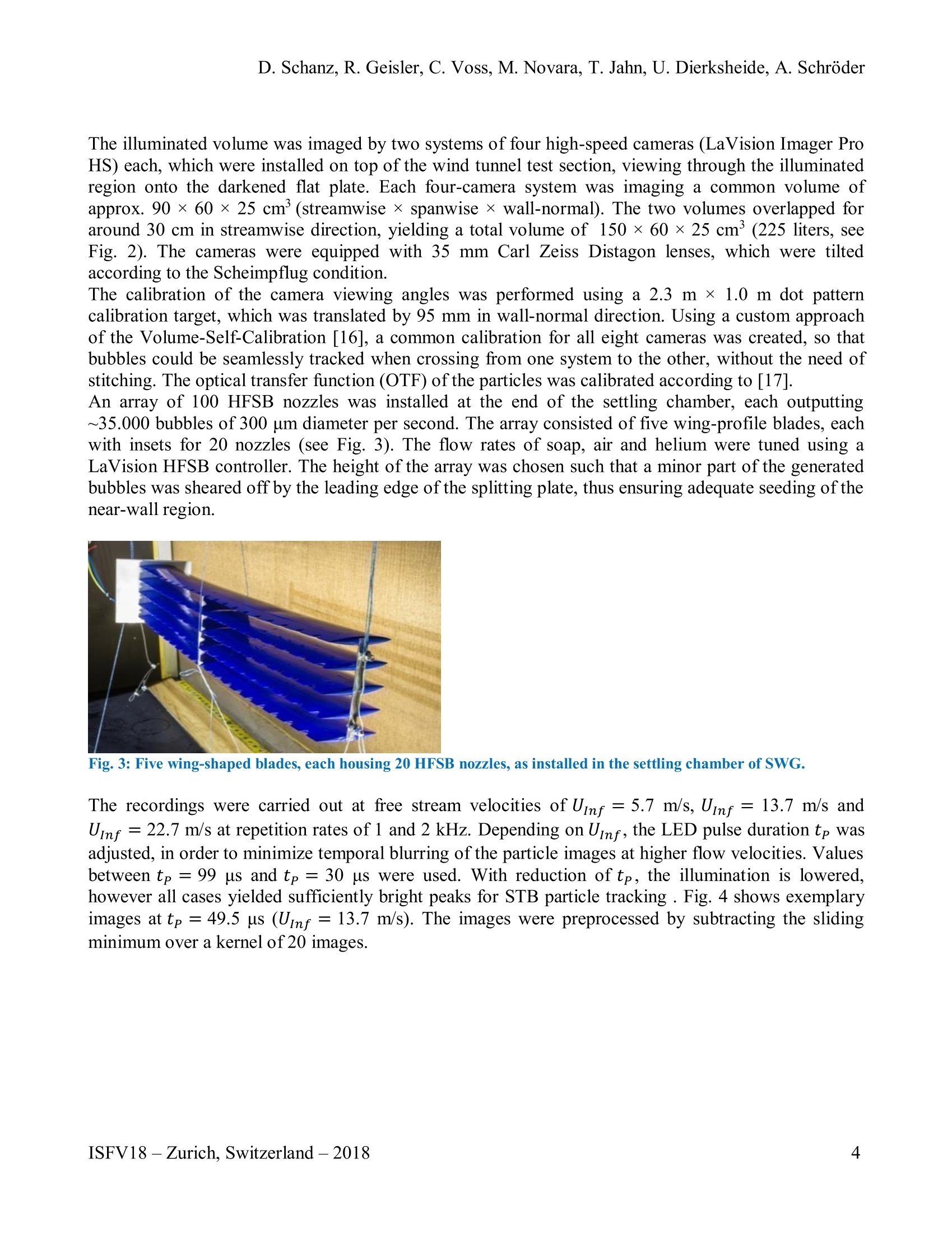
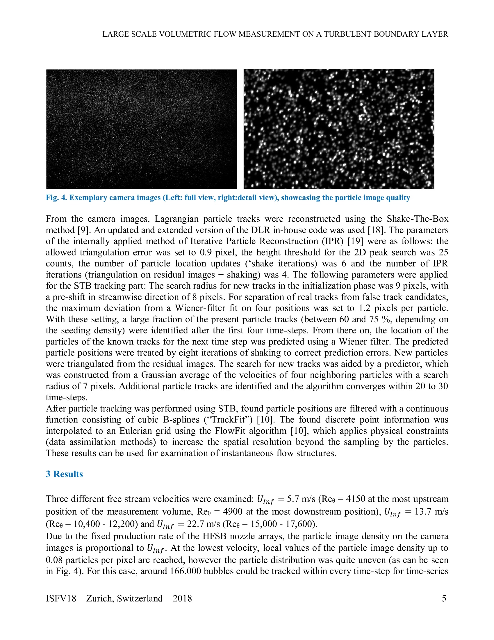
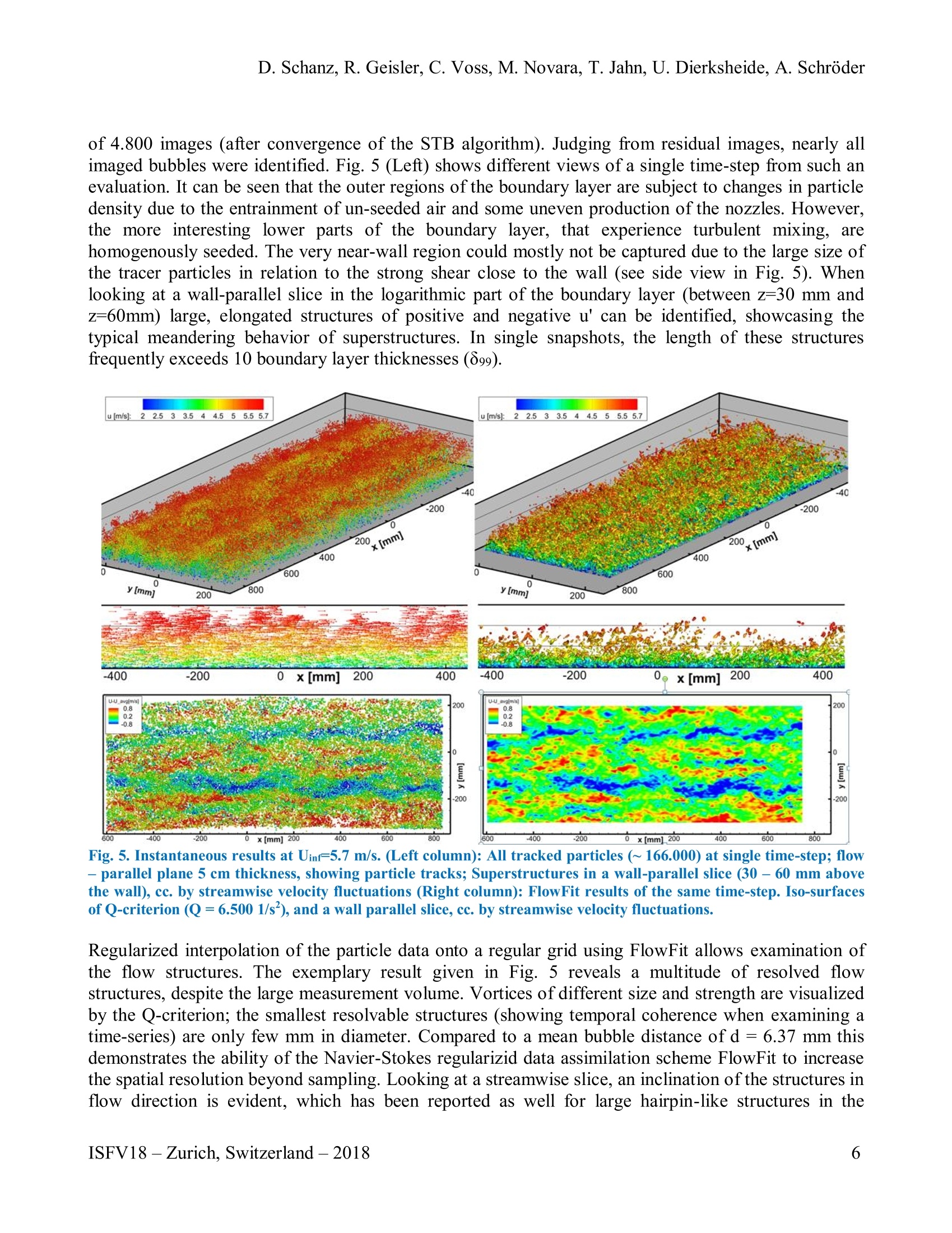
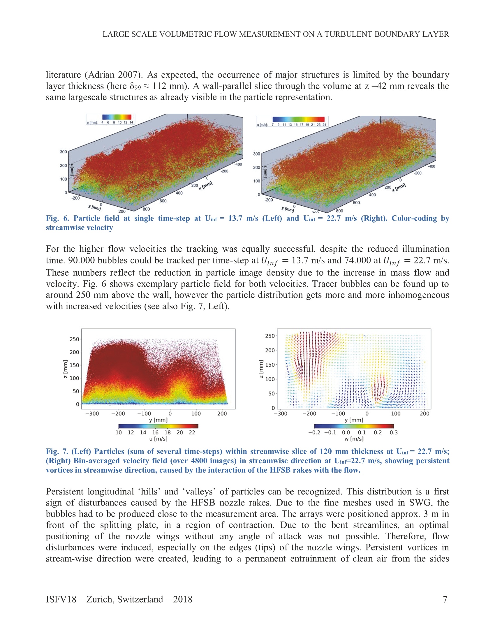
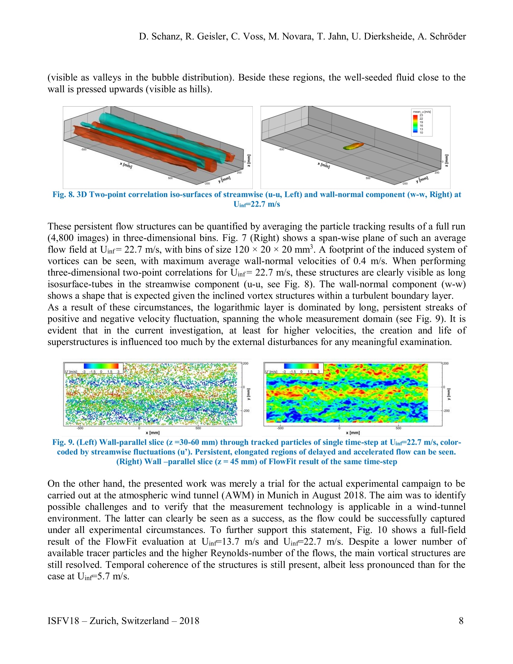
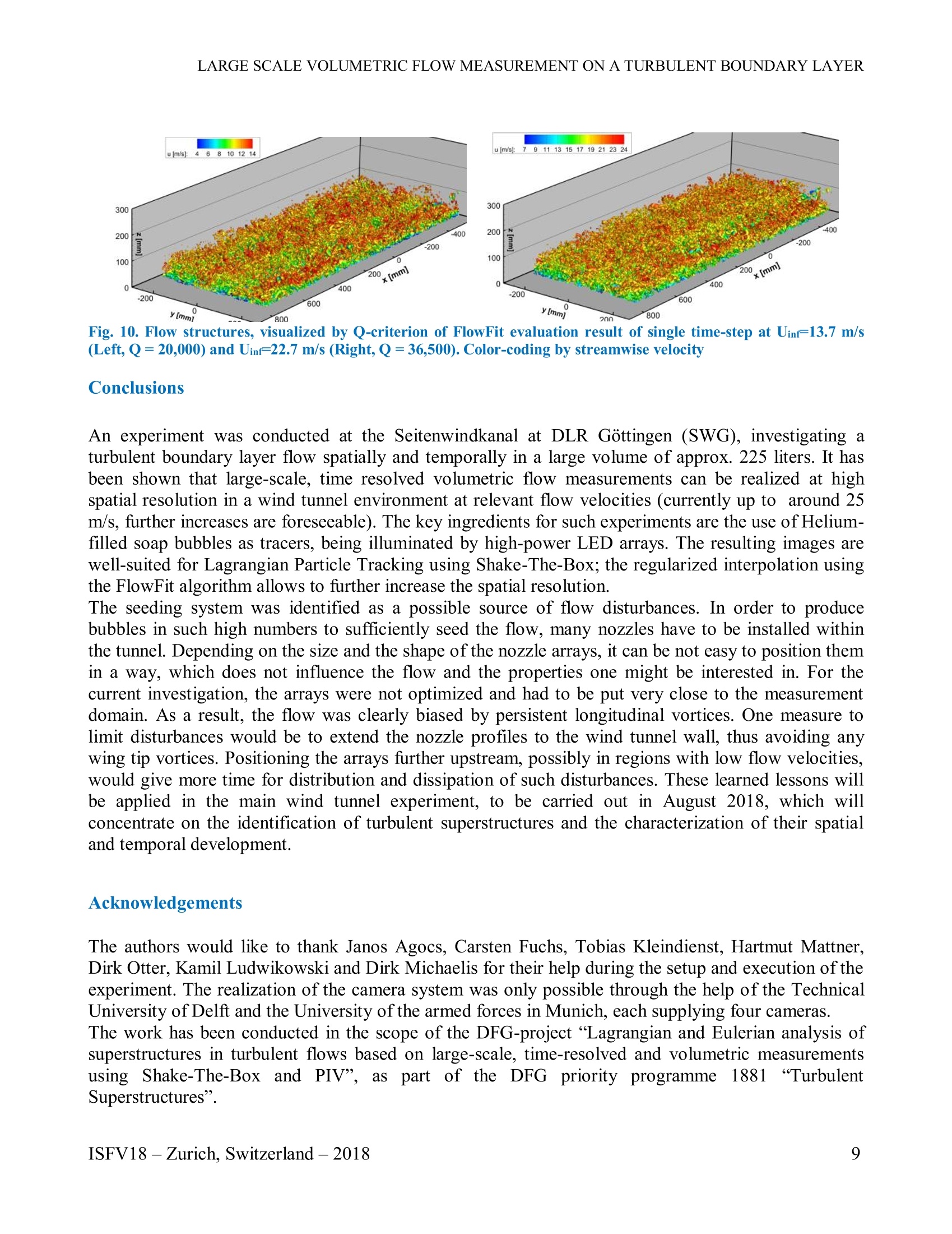
Research Collection 18h International Symposium on Flow VisualizationZurich, Switzerland, June 26-29, 2018 Conference Paper Large scale volumetric flow measurements in a turbulentboundary layer Author[s]:Schanz, Daniel; Geisler, R.; Voss, C.; Novara, M.; Jahn, T.; Dierksheide, U.; Schroder, A. Publication Date: 2018-10-05 Permanent Link: https://doi.org/10.3929/ethz-b-000279208 Rights /License: In Copyright -Non-Commercial Use Permitted → This page was generated automatically upon download from the ETH Zurich Research Collection. For moreinformation please consult the Terms of use. LARGE SCALE VOLUMETRIC FLOW MEASUREMENTS INATURBULENT BOUNDARY LAYER D. Schanz, R. Geisler, C. Voss, M. Novara, T. Jahn', U. Dierksheide, A. Schroder 'German Aerospace Center (DLR), Institute of Aerodynamics and Flow Technology,Department of Experimental Methods, Gottingen, 37073, Germany LaVision GmbH, Gottingen, 37081, Germany Corresponding author: Tel.: +495517092883; Email: daniel.schanz@dlr.de KEYWORDS: Main subjects: turbulent boundary layer, superstructures, flow visualizationFluid: low-speed air flow Visualization method(s): Lagrangian Particle Tracking, data assimilationOther keywords: Shake-The-Box, FlowFit ABSTRACT: The aim ofthis work is to capture the spatiotemporal dynamics oflarge-scale flow structuresin a turbulent boundary layer flow in a volumetric and time-resolved way. The applied means are denseLagrangian Particle Tracking of Helium-Filled Soap Bubbles (HFSBs) using the Shake-The-Box (STB)algorithm and a subsequent interpolation to a regular grid using the physically regularized FlowFit method.The presented experiment was performed as a pre-test to a full campaign to be held in August 2018 at theAtmospheric wind tunnel at the University ofthe armed forces in Munich, Germany. This test demonstratesthe principle applicability ofthe measurement techniques to a low-speed wind tunnel environment and showsthat high spatial accuracy and resolution can be reached despite ofa large measurement volume. Problemswere encountered achieving a homogeneous bubble distribution and in deploying large amounts of bubbles,while not disturbing the flow. 1 Introduction The understanding of the formation and the dynamics of very-large scale coherent structures withinturbulent boundary layers (TBL) and their influence on the wall shear stress is an important researchtopic in aerodynamic flows at high Reynolds numbers not attainable by DNS.[1] showed that eddieswith streamwise lengths of 10-20 8 are present in the logarithmic region of wall-bounded flows bycompiling results from existing measurements and numerical simulations. [2] found streamwiseenergetic modes with wavelengths up to 14 pipe radii within fully developed turbulent pipe flow. Theyaccounted the alignment of packets of hairpin-vortices as responsible for the creation of such structuresand termed them ‘very large scale motion’(VLSM). Indications of the existence of similar flowstructures within the log-region of TBLs were given by [3], as well as [4]. They were able to documentthe existence of long stripes of negative or positive streamwise velocity fluctuations (u’') within thesedomains. Both publications relied on measurements using the method of particle imaging velocimetry(PIV) with a streamwise length of the investigation area around two times the boundary layer thickness(8). Therefore the full extent of the found structures could not be examined. [5] and again [6] confirmedthese results using a similar PIV-setup. Additionally, they performed measurements using a hotwirerake, covering a spanwise distance of more than one 8 with eleven hot-wire probes. By applyingTaylor’s hypothesis on the obtained time-series, they were able to extract quasi-instantaneoussnapshots of the flow structures at several heights above the wall. In many of these snapshots, verylong structures of positive and negative u’can be seen, frequently exceeding a length of 20 8. Theseregions of negative and positive u’typically appear besides each other and show a meandering behavior in spanwise direction. The authors account this meandering to the fact that the length scalesindicated by single-point statistics were much shorter (around 6 8). Due to the large extent of the foundfeatures, the authors termed them ‘superstructures’. As shown by experimental data [7][8], thesesuperstructures seem to directly interact with small-scale structures near the wall (leaving a ‘footprint’).This impact on the conditions near the wall is of particular interest for the wall-shear stress induceddrag production, as the large-scale structures underlie outer scaling (their extent is dependent on 8 andtherefore also dependent on the Reynolds number), while it was assumed that near-wall structures donot. A further examination of the formation and evolution of superstructures in their fully temporal andspatial extension is therefore of major interest for a better understanding of turbulent (wall bounded)flows in general. The aim of this work is to capture the large-scale development of a turbulent boundary layer in a bothvolumetric and time-resolved way. The applied means to achieve this goal are dense LagrangianParticle Tracking of Helium-Filled Soap Bubbles (HFSBs) using the Shake-The-Box (STB) algorithm[9] and a subsequent interpolation to a regular grid using the physically regularized FlowFit method[10]. The presented experiment was performed as a pre-test to a full campaign to be held in August2018 at the atmospheric wind tunnel (AWM) at the University of the armed forces in Munich,Germany. Fig. 1. 3D sketch of the splitting plate, as installed in the Seitenwindkanal Gottingen (SWG) (see right insert). Theleft insert shows a photograph of the plate in the tunnel. The measurement volume is indicated by the green box. 2 Experimental Methods and Setup It has been shown recently that tracking HFSBs in flows up to approx. 20 m/s is possible at highaccuracies and bubble numbers due to the large amounts of light reflected by the bubble surface and theresulting very good image quality [11][12][13]. Illuminating the bubbles with state-of-the-art high power pulsed LED arrays allows for scaling theinstantaneous measurement volume up to the cubic meter range. The tracing fidelity of such bubbleshas been shown to be sufficient for low-speed wind tunnel experiments [14]. Here, the measurement principle was applied to a TBL flow, which was created in the Seitenwindkanalat DLR Gottingen (SWG). To this end, a splitting plate of 7.67 meter length and 2.39 m width wasinstalled in the 9 m long test section of the tunnel (see Fig. 1). A tripping tape was applied right afterthe elliptical leading edge. Close to the end of the splitting plate, a system of four newly developedhigh-power LED arrays [15] was installed on one side of the tunnel, illuminating the plate spanwiseand tangentially over a streamwise length of 1.5 m and a height of approx. 0.25 m (see Fig. 1 and Fig.2). Mirrors were installed on the opposite wind tunnel side wall, back-reflecting the volumetric lightsheet, in order to increase the effective light output. Due to the low opening angle of the LEDs (6°), the light volume remains well confined within the measurement volume. Fig.2. (Left, up) Overview of the LED arrays and cameras installed at SWG; (Right, up) Four LED arrays, installedat the wind tunnel side, illuminating the HFSB inside theTBL flow through a glass window; (Left, down) the camerasystem viewed through the windows in the ceiling of the tunnel. (Right, down) Sketch of the fields of view of twooverlapping four-camera systems, forming one large connected measurement field of 1.5 m length. The illuminated volume was imaged by two systems of four high-speed cameras (LaVision Imager ProHS) each, which were installed on top of the wind tunnel test section, viewing through the illuminatedregion onto the darkened flat plate. Each four-camera system was imaging a common volume ofapprox. 90×60×25 cm(streamwise ×spanwise × wall-normal). The two volumes overlapped foraround 30 cm in streamwise direction, yielding a total volume of 150×60×25 cm’ (225 liters, seeFig. 2). The cameras were equipped with 35 mm Carl Zeiss Distagon lenses, which were tiltedaccording to the Scheimpflug condition. The calibration of the camera viewing angles was performed using a 2.3 m x 1.0 m dot patterncalibration target, which was translated by 95 mm in wall-normal direction. Using a custom approachof the Volume-Self-Calibration [16], a common calibration for all eight cameras was created, so thatbubbles could be seamlessly tracked when crossing from one system to the other, without the need ofstitching. The optical transfer function (OTF) of the particles was calibrated according to [17]. An array of 100 HFSB nozzles was installed at the end of the settling chamber, each outputting~35.000 bubbles of 300 um diameter per second. The array consisted of five wing-profile blades, eachwith insets for 20 nozzles (see Fig. 3). The flow rates of soap, air and helium were tuned using aLaVision HFSB controller. The height of the array was chosen such that a minor part of the generatedbubbles was sheared off by the leading edge of the splitting plate, thus ensuring adequate seeding of thenear-wall region. Fig. 3: Five wing-shaped blades, each housing 20 HFSB nozzles, as installed in the settling chamber of SWG. The recordings were carried out at free stream velocities of Uinf =5.7 m/s, Umnf = 13.7 m/s andUinf =22.7 m/s at repetition rates of 1 and 2 kHz. Depending on Uinf, the LED pulse duration tp wasadjusted, in order to minimize temporal blurring of the particle images at higher flow velocities. Valuesbetween tp =99 us and tp =30 us were used. With reduction of tp, the illumination is lowered,however all cases yielded sufficiently bright peaks for STB particle tracking. Fig. 4 shows exemplaryimages at tp =49.5 us (Uinf =13.7 m/s). The images were preprocessed by subtracting the slidingminimum over a kernel of 20 images. Fig. 4. Exemplary camera images (Left: full view, right:detail view), showcasing the particle image quality From the camera images, Lagrangian particle tracks were reconstructed using the Shake-The-Boxmethod [9]. An updated and extended version of the DLR in-house code was used [18]. The parametersof the internally applied method of Iterative Particle Reconstruction (IPR) [19] were as follows: theallowed triangulation error was set to 0.9 pixel, the height threshold for the 2D peak search was 25counts, the number of particle location updates (‘shake iterations) was 6 and the number of IPRiterations (triangulation on residual images + shaking) was 4. The following parameters were appliedfor the STB tracking part: The search radius for new tracks in the initialization phase was 9 pixels, witha pre-shift in streamwise direction of 8 pixels. For separation of real tracks from false track candidates,the maximum deviation from a Wiener-filter fit on four positions was set to 1.2 pixels per particle.With these setting, a large fraction of the present particle tracks (between 60 and 75 %, depending onthe seeding density) were identified after the first four time-steps. From there on, the location of theparticles of the known tracks for the next time step was predicted using a Wiener filter. The predictedparticle positions were treated by eight iterations of shaking to correct prediction errors. New particleswere triangulated from the residual images. The search for new tracks was aided by a predictor, whichwas constructed from a Gaussian average of the velocities of four neighboring particles with a searchradius of 7 pixels. Additional particle tracks are identified and the algorithm converges within 20 to 30time-steps. After particle tracking was performed using STB, found particle positions are filtered with a continuousfunction consisting of cubic B-splines (“TrackFit") [10]. The found discrete point information wasinterpolated to an Eulerian grid using the FlowFit algorithm [10], which applies physical constraints(data assimilation methods) to increase the spatial resolution beyond the sampling by the particles.These results can be used for examination of instantaneous flow structures. Three different free stream velocities were examined: Uinf = 5.7 m/s (Re:=4150 at the most upstreamposition of the measurement volume, Ree=4900 at the most downstream position), Uif = 13.7 m/s(Re一=10,400-12,200) and Uinf=22.7 m/s (Ree=15,000-17,600). Due to the fixed production rate of the HFSB nozzle arrays, the particle image density on the cameraimages is proportional to Uinf. At the lowest velocity, local values of the particle image density up to0.08 particles per pixel are reached, however the particle distribution was quite uneven (as can be seenin Fig. 4). For this case, around 166.000 bubbles could be tracked within every time-step for time-series of 4.800 images (after convergence of the STB algorithm). Judging from residual images, nearly allimaged bubbles were identified. Fig. 5 (Left) shows different views of a single time-step from such anevaluation. It can be seen that the outer regions of the boundary layer are subject to changes in particledensity due to the entrainment of un-seeded air and some uneven production of the nozzles. However,the more interesting lower parts of the boundary layer, that experience turbulent mixing, arehomogenously seeded. The very near-wall region could mostly not be captured due to the large size ofthe tracer particles in relation to the strong shear close to the wall (see side view in Fig. 5). Whenlooking at a wall-parallel slice in the logarithmic part of the boundary layer (between z=30 mm andz=60mm) large, elongated structures of positive and negative u' can be identified, showcasing thetypical meandering behavior of superstructures. In single snapshots, the length of these structuresfrequently exceeds 10 boundary layer thicknesses (899). Fig. 5. Instantaneous results at Uinr=5.7 m/s. (Left column): All tracked particles (~166.000) at single time-step; flow- parallel plane 5 cm thickness, showing particle tracks; Superstructures in a wall-parallel slice (30- 60 mm abovethe wall), cc. by streamwise velocity fluctuations (Right column): FlowFit results of the same time-step. Iso-surfacesof Q-criterion (Q=6.500 1/s), and a wall parallel slice, cc. by streamwise velocity fluctuations. Regularized interpolation of the particle data onto a regular grid using FlowFit allows examination ofthe flow structures. The exemplary result given in Fig. 5 reveals a multitude of resolved flowstructures, despite the large measurement volume. Vortices of different size and strength are visualizedby the Q-criterion; the smallest resolvable structures (showing temporal coherence when examining atime-series) are only few mm in diameter. Compared to a mean bubble distance of d=6.37 mm thisdemonstrates the ability of the Navier-Stokes regularizid data assimilation scheme FlowFit to increasethe spatial resolution beyond sampling. Looking at a streamwise slice, an inclination of the structures inflow direction is evident, which has been reported as well for large hairpin-like structures in the literature (Adrian 2007). As expected, the occurrence of major structures is limited by the boundarylayer thickness (here 899 ≈112 mm). A wall-parallel slice through the volume at z =42 mm reveals thesame largescale structures as already visible in the particle representation. streamwise velocity For the higher flow velocities the tracking was equally successful, despite the reduced illuminationtime. 90.000 bubbles could be tracked per time-step at Umnf = 13.7 m/s and 74.000 at Uinf =22.7 m/s.These numbers reflect the reduction in particle image density due to the increase in mass flow andvelocity. Fig. 6 shows exemplary particle field for both velocities. Tracer bubbles can be found up toaround 250 mm above the wall, however the particle distribution gets more and more inhomogeneouswith increased velocities (see also Fig. 7,Left). Fig. 7. (Left) Particles (sum of several time-steps) within streamwise slice of 120 mm thickness at Uinf=22.7 m/s;(Right) Bin-averaged velocity field (over 4800 images) in streamwise direction at Uinf=22.7 m/s, showing persistentvortices in streamwise direction, caused by the interaction of the HFSB rakes with the flow. Persistent longitudinal‘hills’and ‘valleys’of particles can be recognized. This distribution is a firstsign of disturbances caused by the HFSB nozzle rakes. Due to the fine meshes used in SWG, thebubbles had to be produced close to the measurement area. The arrays were positioned approx. 3 m infront of the splitting plate, in a region of contraction. Due to the bent streamlines, an optimalpositioning of the nozzle wings without any angle of attack was not possible. Therefore, flowdisturbances were induced, especially on the edges (tips) of the nozzle wings. Persistent vortices instream-wise direction were created, leading to a permanent entrainment of clean air from the sides Fig.8.3D Two-point correlation iso-surfaces of streamwise (u-u, Left) and wall-normal component (w-w,Right) atUint=22.7 m/s These persistent flow structures can be quantified by averaging the particle tracking results of a full run(4,800 images) in three-dimensional bins. Fig. 7 (Right) shows a span-wise plane of such an averageflow field at Uinf=22.7 m/s, with bins of size 120 ×20×20mm’. A footprint of the induced system ofvortices can be seen, with maximum average wall-normal velocities of 0.4 m/s. When performingthree-dimensional two-point correlations for Uinf= 22.7 m/s, these structures are clearly visible as longisosurface-tubes in the streamwise component (u-u, see Fig. 8). The wall-normal component (w-w)shows a shape that is expected given the inclined vortex structures within a turbulent boundary layer.As a result of these circumstances, the logarithmic layer is dominated by long, persistent streaks ofpositive and negative velocity fluctuation, spanning the whole measurement domain (see Fig. 9). It isevident that in the current investigation, at least for higher velocities, the creation and life of superstructures is influenced too much by the external disturbances for any meaningful examination. Fig. 9. (Left) Wall-parallel slice (z =30-60 mm) through tracked particles of single time-step at Uinr=22.7 m/s, color-coded by streamwise fluctuations (u’). Persistent, elongated regions of delayed and accelerated flow can be seen.(Right) Wall -parallel slice (z =45 mm) of FlowFit result of the same time-step On the other hand, the presented work was merely a trial for the actual experimental campaign to becarried out at the atmospheric wind tunnel (AWM) in Munich in August 2018. The aim was to identifypossible challenges and to verify that the measurement technology is applicable in a wind-tunnelenvironment. The latter can clearly be seen as a success, as the flow could be successfully capturedunder all experimental circumstances. To further support this statement, Fig. 10 shows a full-fieldresult of the FlowFit evaluation at Uinf=13.7 m/s and Uinf=22.7 m/s. Despite a lower number ofavailable tracer particles and the higher Reynolds-number of the flows, the main vortical structures arestill resolved. Temporal coherence of the structures is still present, albeit less pronounced than for thecase at Uinf=5.7 m/s. Fig.10. Flow structures, visualized by Q-criterion of FlowFit evaluation result of single time-step at Uinr=13.7 m/s(Left, Q=20,000) and Uinf=22.7 m/s (Right, Q=36,500).Color-coding by streamwise velocity Conclusions An experiment was conducted at the Seitenwindkanal at DLR Gottingen (SWG), investigating aturbulent boundary layer flow spatially and temporally in a large volume of approx. 225 liters. It hasbeen shown that large-scale, time resolved volumetric flow measurements can be realized at highspatial resolution in a wind tunnel environment at relevant flow velocities (currently up to around 25m/s, further increases are foreseeable). The key ingredients for such experiments are the use of Helium-filled soap bubbles as tracers, being illuminated by high-power LED arrays. The resulting images arewell-suited for Lagrangian Particle Tracking using Shake-The-Box; the regularized interpolation usingthe FlowFit algorithm allows to further increase the spatial resolution. The seeding system was identified as a possible source of flow disturbances. In order to producebubbles in such high numbers to sufficiently seed the flow, many nozzles have to be installed withinthe tunnel. Depending on the size and the shape of the nozzle arrays, it can be not easy to position themin a way, which does not influence the flow and the properties one might be interested in. For thecurrent investigation, the arrays were not optimized and had to be put very close to the measurementdomain. As a result, the flow was clearly biased by persistent longitudinal vortices.One measure tolimit disturbances would be to extend the nozzle profiles to the wind tunnel wall, thus avoiding anywing tip vortices. Positioning the arrays further upstream, possibly in regions with low flow velocities,would give more time for distribution and dissipation of such disturbances. These learned lessons willbe applied in the main wind tunnel experiment, to be carried out in August 2018, which willconcentrate on the identification of turbulent superstructures and the characterization of their spatialand temporal development. Acknowledgements The authors would like to thank Janos Agocs, Carsten Fuchs, Tobias Kleindienst, Hartmut Mattner,Dirk Otter, Kamil Ludwikowski and Dirk Michaelis for their help during the setup and execution of theexperiment. The realization of the camera system was only possible through the help of the TechnicalUniversity of Delft and the University of the armed forces in Munich, each supplying four cameras.The work has been conducted in the scope of the DFG-project“Lagrangian and Eulerian analysis ofsuperstructures in turbulent flows based on large-scale, time-resolved and volumetric measurementsusing Shake-The-Box ;andPIV”,aspart of the DFG priority programme1881“TurbulentSuperstructures”. ( R eferences ) ( [1] Jimenez J (1998), The Largest Scales of Turbulent Wall Flows, CTR Annual Research Briefs : 137-54, Univer s ity, Stanford ) ( [2] K F im KC, Adrian RJ (1999), Very large-scale motion in the outer layer. Phys. Fluid s 11:417-422 ) ( [3] Tomkins CD, Ad r ian R. J (2003), Sp a nwise structure and sc a le growth in turbulent boundary la y ers.J. F l uid M e ch.490:37-74 ) ( [4] G ( anapathisubramani, B., L o ngmire, E.K., Marusic, I. ( 2 003), Characteristics of vortex packets in turbulent boundarylayers. J. Flui d Mech. 478: 35-46 ) ( [5] H utchins N, M a rusic I ( 2 0 07), Ev i dence of ver y long mean d ering featu r es in th e l o gar i thmic regio n of turbulent b oundary l a yers. J. Fluid Mech. 579:1-28 ) ( [6] Marusic I , McKeon B J , Monkewitz PA, Na g ib HM, Smits AJ, Sreenivasan KR (2010),Wall-bounded turbulent flows at high Reynolds numbers: recent a dvances and key issues, Phys. Fluids 22, 065103 ) ( [7] H I utchins N, Monty JP, G a napathisubramani B, Ng HCH, Maru s ic I (20 1 1 ), T h ree-dimensional stru c ture of a h i g h - Reynolds-number turbulent boundary layer, J . Fluid Mech. 673: 255-285, DOI : 10.1017/ S0022112010006245 ) ( [8] d q e S ilva CM, Gnanamanickam EP, Atk i nson C, Buc h mann NA, H u tchins N, Sor i a J , Marus i c I (2014), High spati a lrange v elocity measurements in a h i gh Reynolds number turbulent boundary layer, Phys i cs of F l uids, 26, 025117, DOI:10.1063/1.4866458 ) ( [9] Schanz D, G e semann S, Schroder A ( 2 01 6 ) Shak e -The-Box: Lagrangian particle track i ng at hi g h parti c le imag e densities. Exp Fluids, 5 7(5) ) ( [10]Gesemann S, Huhn F, Schanz D, Sch r oder A (201 6 ): From noisy particle tracks to velocity, ac c eleration and pressurefields using B-splines and penalties. 18th Int. Symp. on Appl. o f Laser a nd Imaging Te c h. to Fl u id Me c h. Lis b on,Portugal, July 4 - 72016 ) ( [1 1 ]Schanz D, Huhn F, Gesemann S, Dierksheide U, van de Meerendonk R, Mano v ski P, Sc h ro d er A (2016) Towards high-resolution 30 f low field measurements at t h e cubic meter scale. 1 8 th I n t. S ymp. on Appl. of Laser and Imaging Tech. toFluid Mech. Lisbon, Portugal, July4- 7 2016 ) ( [12]Huhn F, S chanz D, Gesemann S, Dierksheide U , v a n d e M e erendonk R, Sc h roder A ( 2017) Large-scale volumetric flow m easurement in a pure thermal plume by dense tracking of helium-lied soap bubbles, Exp. Fluids 58:116. ) ( [13]Huhn, F., Schanz, D.,Manovski, P. et al. (2018) Exp Fluids 59: 81. http s://d oi .org/10.1007/s0034 8-018-2533-0 ) ( [14]Scarano F , Ghaemi S, Caridi GAC, Bos b ach J, Dierksheide U, Sciacchitano A (2015 ) On the us e of helium-filled soap bubbles for large-scale tomographic PIV in wind tunnel experiments; Exp. Flui d s 56:42 ) ( [15]Stasicki B, Schroder A, Boden F, Ludwikowski K ( 2017) High-power LED l ight sources for opti c al mea s urement systems operated i n continuous and overdriven pu l sed modes, Optical Measurement Systems for Ind u strial Inspection X10329, 103292J ) ( [16] Wieneke B (2008) Volume se l f-calibration f or 3D particle image velocimetry. Exp Fluids, 45:549-556 ) ( [17] Schanz D, Gesemann S, S c hroder A, Wieneke B, Novara M (2013) No n -uniform optical trans f er functions in particleimaging: calibration and application to tomographic reconstruction. Meas Sci Technol 24 024009 ) ( [18]Jahn T (2017) Volumetrische Stromungsvermessung: Eine Imp l ementierung von Shak e -The-Box. Masterarbeit, Georg-August-Universitat Gottingen & DLR Gottingen. ) ( [19]Wieneke B (2013) Iterative reconstruction of volumetric particle distribution . Meas. Sci. Technol. 24:024008 ) ISFV Zurich, Switzerland- The aim of this work is to capture the spatiotemporal dynamics of large-scale flow structures in a turbulent boundary layer flow in a volumetric and time-resolved way. The applied means are dense Lagrangian Particle Tracking of Helium-Filled Soap Bubbles (HFSBs) using the Shake-The-Box (STB) algorithm and a subsequent interpolation to a regular grid using the physically regularized FlowFit method. The presented experiment was performed as a pre-test to a full campaign to be held in August 2018 at the Atmospheric wind tunnel at the University of the armed forces in Munich, Germany. This test demonstratesthe principle applicability of the measurement techniques to a low-speed wind tunnel environment and shows that high spatial accuracy and resolution can be reached despite of a large measurement volume. Problems were encountered achieving a homogeneous bubble distribution and in deploying large amounts of bubbles, while not disturbing the flow.
确定

还剩9页未读,是否继续阅读?

产品配置单


北京欧兰科技发展有限公司为您提供《湍流边界层中3D3C 流场 抖盒子STB检测方案(CCD相机)》,该方案主要用于航空中3D3C 流场 抖盒子STB检测,参考标准--,《湍流边界层中3D3C 流场 抖盒子STB检测方案(CCD相机)》用到的仪器有LaVision HighSpeedStar 高帧频相机、体视层析粒子成像测速系统(Tomo-PIV)、LaVision DaVis 智能成像软件平台
推荐专场
CCD相机/影像CCD
更多


相关方案
更多
该厂商其他方案
更多