


采用LaVision的同轴体视速度测量系统-机器人式体视PIV对风洞中的球体和假人的流场进行了测量,并通过流场数据获得了表面压力的可视化信息。
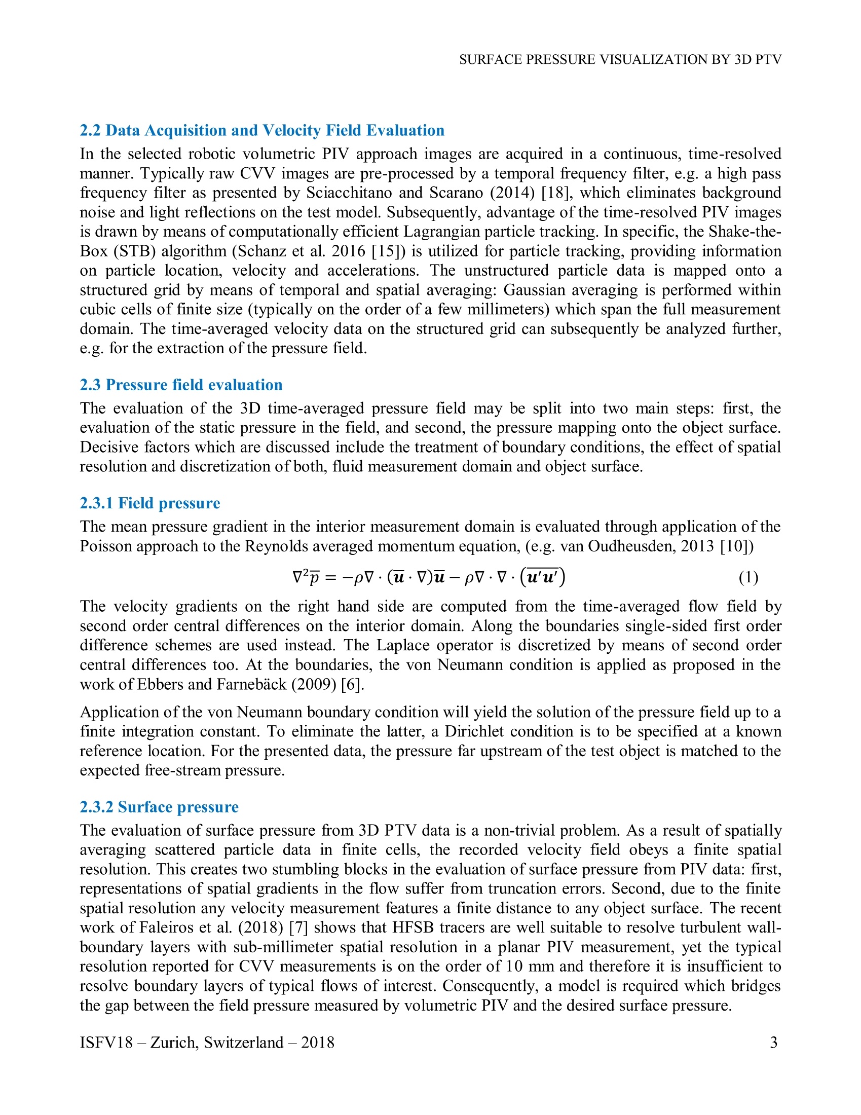
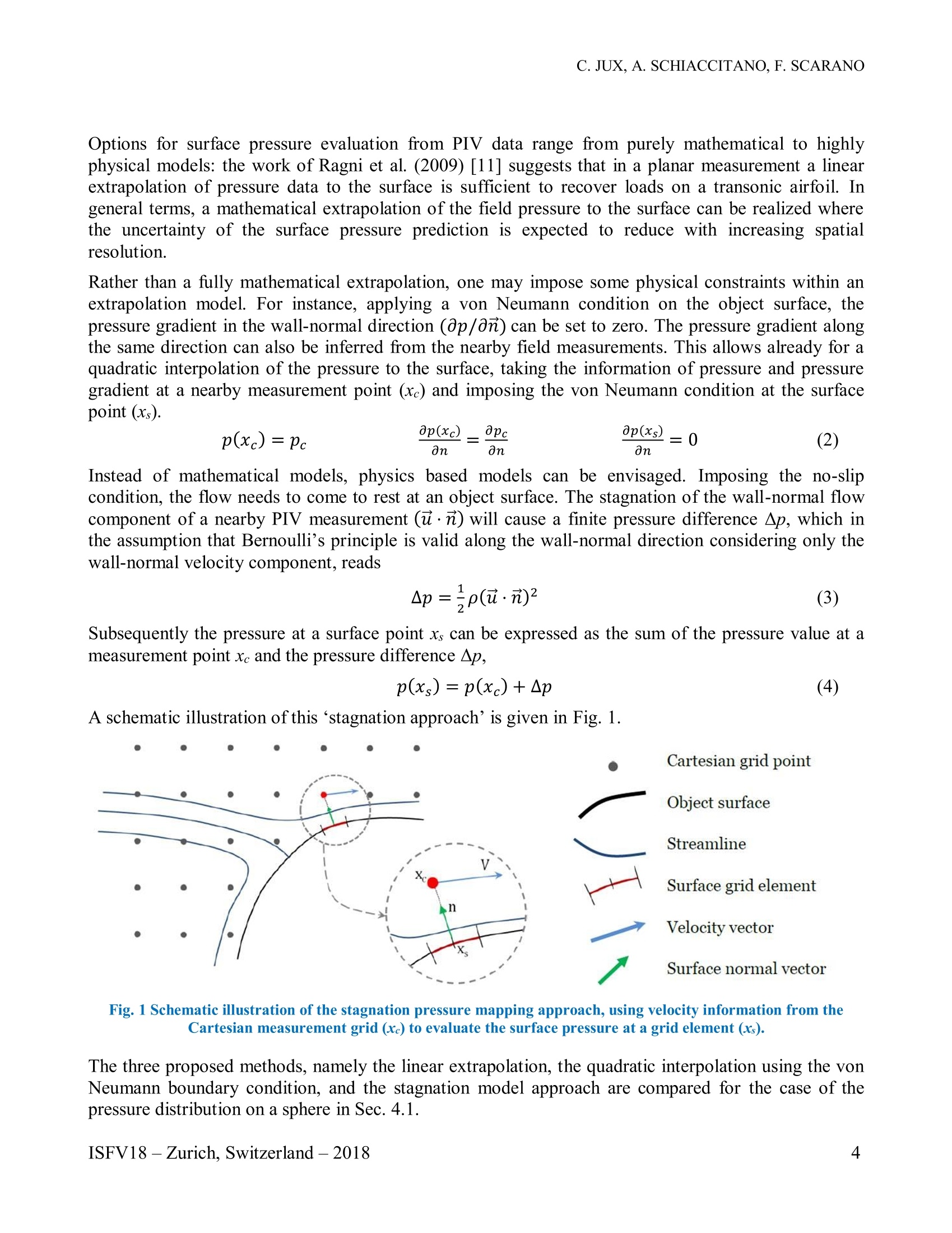
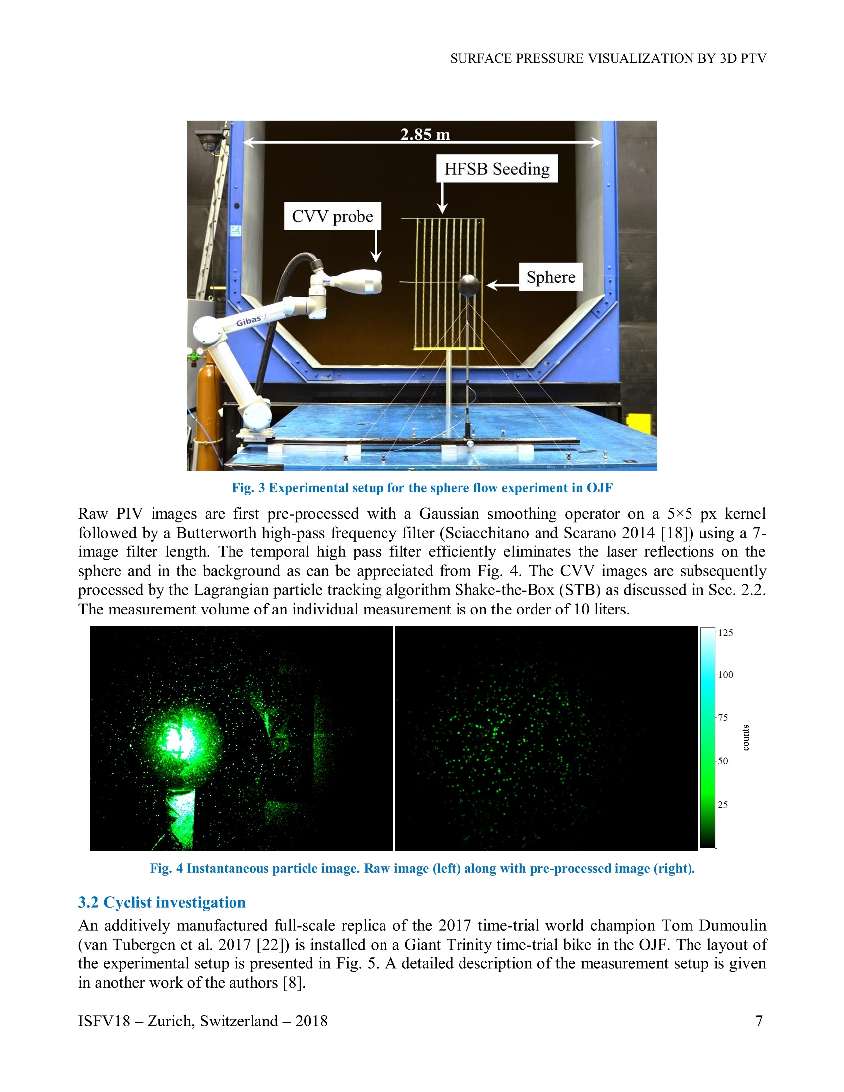
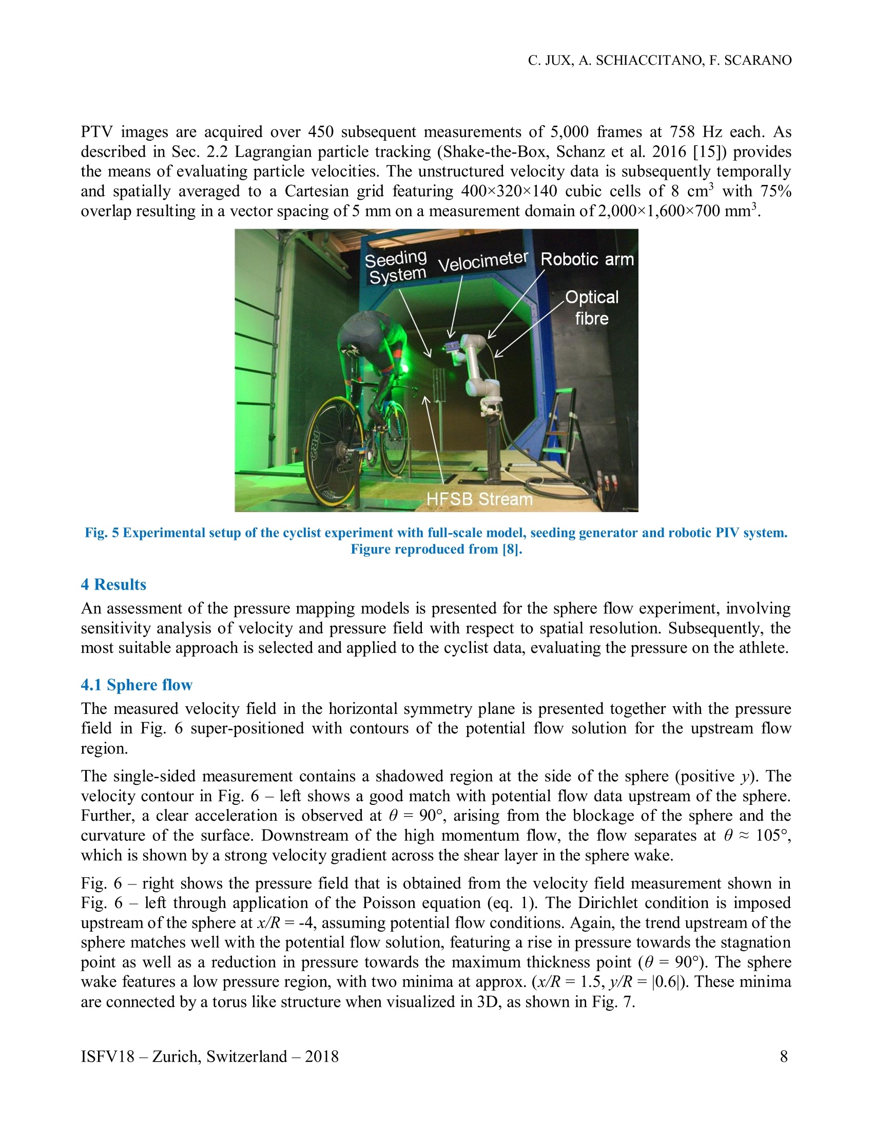
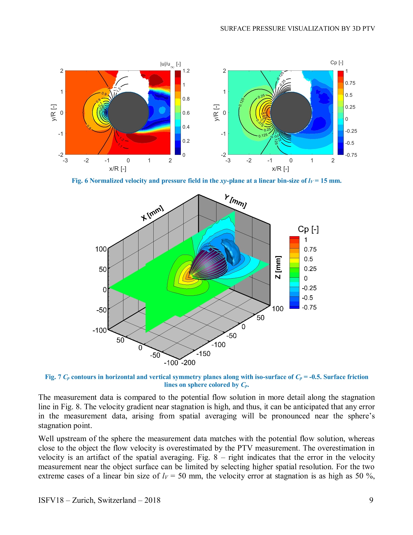
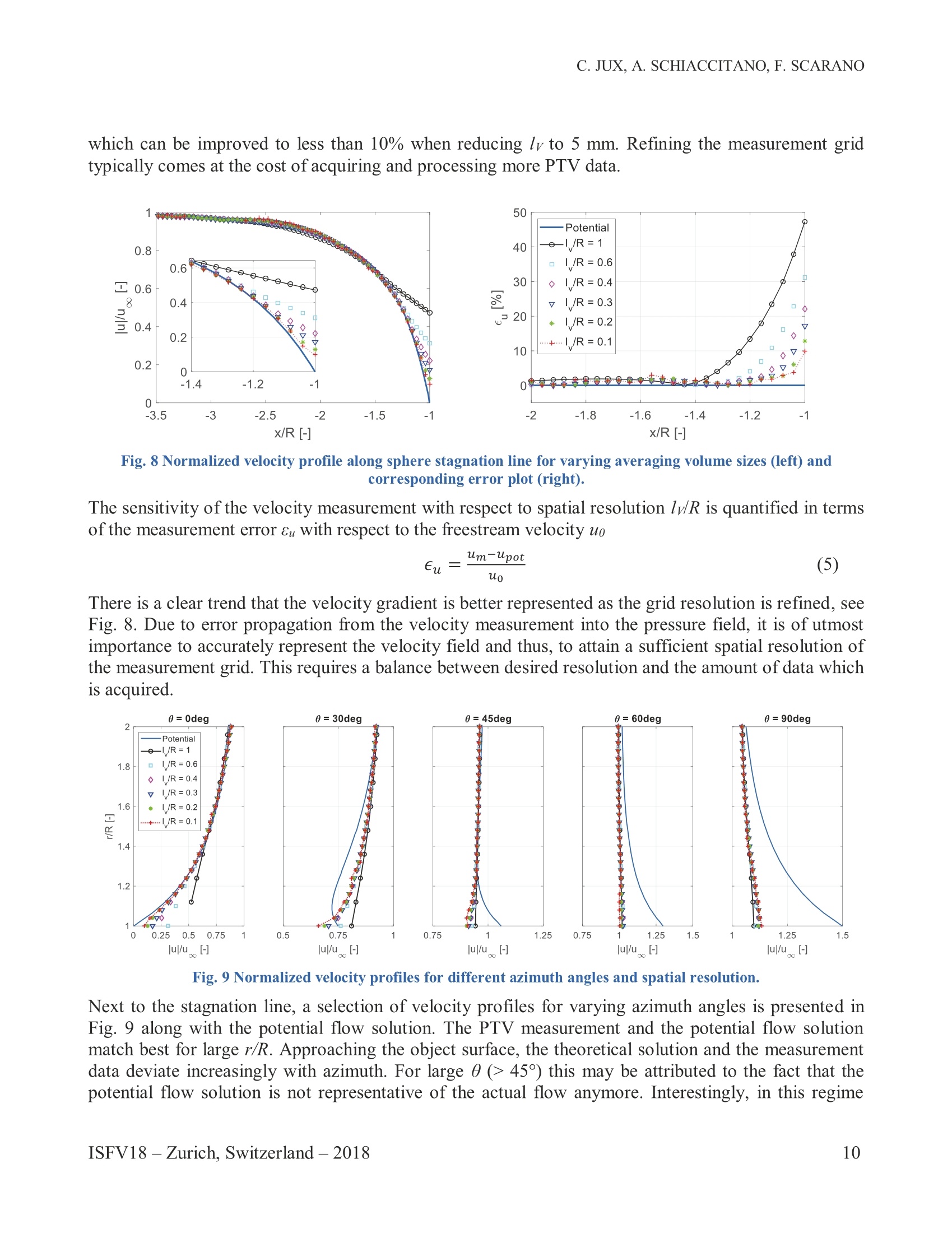
方案详情

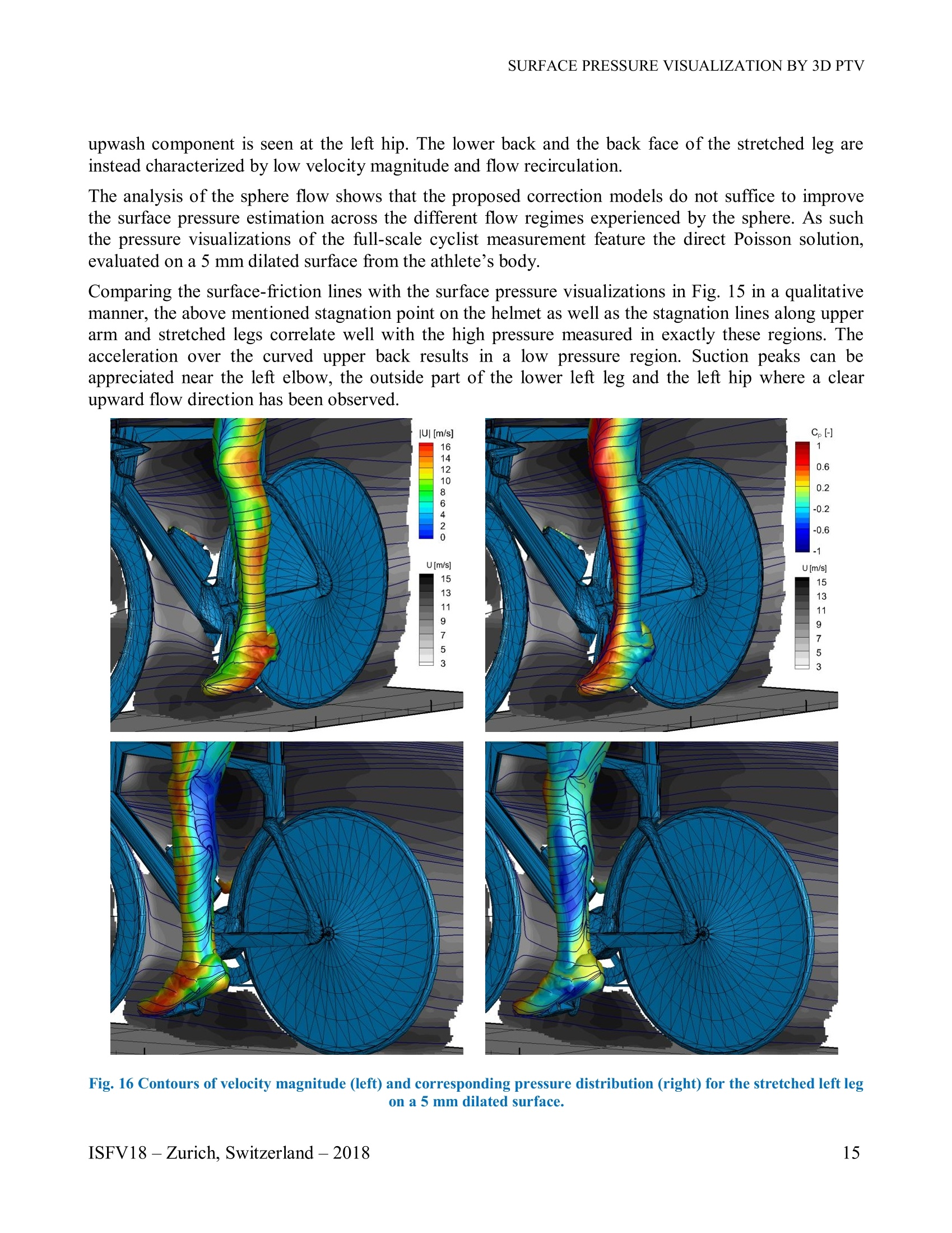
Research Collection 18* International Symposium on Flow VisualizationZurich, Switzerland, June 26-29, 2018 Conference Paper Surface pressure visualization by 3D PTV Author(s]: Jux, C.; Sciacchitano, A.; Scarano,F. Publication Date: 2018-10-05 Permanent Link: https://doi.org/10.3929/ethz-b-000279192 → Rights/License: In Copyright-Non-Commercial Use Permitted → This page was generated automatically upon download from the ETH Zurich Research Collection. For moreinformation please consult the Terms of use. SURFACE PRESSURE VISUALIZATION BY3D PTV C. Juxl,, A. Sciacchitano', F. Scarano Faculty of Aerospace Engineering, TU Delft, 2629 HS Delft, The Netherlands‘Corresponding author: Tel.:+49 162 69 20 198; Email: C.Jux@tudelft.nl KEYWORDS: Main subjects: Surface pressure visualization, Large-scale 3D PTV Fluid: Low speed flows, Aerodynamics Visualization method(s): Coaxial volumetric velocimetry, Robotic volumetric PIV Other keywords: Cycling aerodynamics, Large-scale PIV, Bluff body flows, 3D PTV ABSTRACT: Some recent trends in the development of PIV techniques are leading to the realization ofvelocity measurement at large scale. Moreover, methods for evaluating the fluid flow pressure from PIV datahave been successfully demonstrated at small scale and for simple geometries. Methods for quantitativevisualization of surface flow properties such as skin-friction and pressure are comparatively less developed,despite the great interest for the aerodynamic insight they provide for the study of the flow around 3Dcomplexobjects. The accuracy of the pressure evaluation at the surface is inquired in this work by dedicated measurementsover a sphere at Rea =8×10. The measurements made with robotic PIV are compared to direct surfacepressure measurements. The solution of the Reynolds averaged momentum equations is performed with thePoisson problem formulation and the results are compared with potential flow theory and some simplifiedmodels. The accuracy of stagnation pressure depends upon the measurement resolution. Instead, the suctionpeak region is generally underestimated. The pressure in the separated region is retrieved with sufficientaccuracv. The surface flow properties visualization of a time-trialing full-scale cyclist replica at 14 m/s (Re =5.5×10)is performed as a demonstration of the above method to a complex 3D problem at large scale. The dataobtained with the robotic PIV technique is analyzed in close proximity of the solid surface and the skinfriction lines ofthe time averaged velocity field are inspected. The topological analysis ofthe skin frictionlines yields clearly the evolution ofthe flow around the body segments returning the details of the separatedflow regions and local recirculation zones. The analysis of the surface pressure distribution yields results inaccordance with the skin-friction lines, the outer flow velocity field as well as the vortex topology. 1Introduction The recent introduction of coaxial volumetric velocimetry (CVV) by Schneiders et al. (2018) [16] hasgiven impetus to three dimensional velocity field measurements around large and complex geometriesofrelevance for many fields of aerodynamics. The authors (Jux et al. 2018) [8] have coupled CVV witha robotic manipulation system to realize volumetric PTV measurements around a full-scale cyclistmodel. The measurements rely upon Helium filled soap bubbles (HFSB) [14] as flow tracers known fortheir high scattering intensity. The introduction of these three technologies, namely HFSB, CVV androbotic volumetric PIV are motivated by the desire of acquiring volumetric airflow measurements on alarge scale. The trend towards such large-scale volumetric PIV studies is recognized in a number ofrecent studies such as in the work of Caridi et al. (2016) [4] on the tip vortex of a vertical axis windturbine (measurement volume, V= 40×20×15 cm), that of Rius Vidales (2016) [13] on the bi-stablewake structure of a frigate ship model (V=45×25×11 cm’), the cyclist wake analysis of Sciacchitano etal. (2018) [19] (V=162×100×5 cm’) or the robotic volumetric PIV study of Martinez Gallar et al.(2018) [9] on the wake flow of a flapping-wing micro air vehicle (V=50x40×30 cm). The studies mentioned above demonstrated the feasibility of large-scale volumetric velocity fieldmeasurements. A second trend in PIV developments is the evaluation of pressure from (3D) PIV data as highlighted in a review by van Oudheusden (2013) [10]. The tomographic PIV study of Schneiderset al. (2016) [17] on the flow downstream of a truncated cylinder is the first study that reports the useof large-scale (i.e. using HFSB as tracers) volumetric PIV to determine the flow field pressure. Thestudy, is limited to the analysis of the pressure close to the flat plate downstream of the cylinder andexcellent agreement is reported for the time-averaged pressure with respect to pressure taps. The evaluation of the flow field pressure over the curved surface of an airfoil has been addressed in theworks ofRagni and coauthors (Ragni et al. 2009, 2012)[11,12], however, with planar PIV. The resultsindicated that a good accuracy can be achieved in general, provided that the measurements areperformed at good spatial resolution. A pronounced discrepancy in regions with strong local curvatureand gradient of pressure was ascribed to insufficient spatial resolution. Volumetric robotic PIV typically offers lower spatial resolution than the typical measurements with theplanar technique. Nonetheless, volumetric measurements allow to map the velocity field over complexsurfaces, which makes it interesting for applications in the aerodynamic study of 3D objects such as forinstance in sports. One of the limitations of pressure evaluation from velocity data arises from the spatial resolutionlimited by the data density. Typically PIV/PTV measurements are spatially averaged over a smallvolume,which corresponds to the cross-correlation window in PIV and to the three-dimensional binemployed for the computation of the velocity statistics in 3D PTV. The distance between adjacentvelocity vectors is typically a fraction (25% to 100%) of the volume linear dimension lv. Consequently,any measured spatial gradient suffers from filtering effects. Furthermore, the limited spatial resolution,imposes a finite distance from the solid surface, thus complicating the evaluation of the flow fieldvariables at the surface. The present work addresses the latter issue and discusses options to evaluatethe surface-pressure on solid objects based on the near flow velocity field. The proposed methods of surface pressure evaluation from PIV data can be categorized in three types:purely mathematical models which extrapolate the field pressure to the surface, physical models whichleverage knowledge of the flow behavior, and hybrid models which impose some physical constraintsin a mathematical mapping model. The theoretical discussion is accompanied by two wind tunnel experiments to validate the findings andto demonstrate the potential of the presented methodology in large-scale aerodynamic experiments. 2Methods The basic principles of robotic volumetric PIV are summarized hereafter, before addressing theprocedures ofevaluating pressure in the field and on an object surface in Sec. 2.3. 2.1 Principles of robotic volumetric PIV Details on the working principles of robotic volumetric PIV can be found in the work of Jux et al.(e 112018) [8]. The technique utilizes the compactness of coaxial volumetric velocimetry (Schneiders et al.2018 [16]), a low tomographic aperture imaging system which greatly enhances optical access involumetric PIV approaches by aligning imaging and illumination direction and which lends itself wellto robotic manipulation. The CVV system requires a calibration at start of measurement, consisting of apinhole model calibration (Soloff et al. 1997 [20]) and a volume self-calibration (Wieneke 2008 [23]).Subsequently, the CVV probe can be manipulated by a robotic arm, allowing for rapid acquisitions oftime-averaged flow field data by a volume scanning approach. 2.2 Data Acquisition and Velocity Field Evaluation In the selected robotic volumetric PIV approach images are acquired in a continuous, time-resolvedmanner. Typically raw CVV images are pre-processed by a temporal frequency filter, e.g. a high passfrequency filter as presented by Sciacchitano and Scarano (2014) [18], which eliminates backgroundnoise and light reflections on the test model. Subsequently, advantage of the time-resolved PIV imagesis drawn by means of computationally efficient Lagrangian particle tracking. In specific, the Shake-the-Box (STB) algorithm (Schanz et al. 2016 [15]) is utilized for particle tracking, providing informationon particle location, velocity and accelerations.The unstructured particle data is mapped onto astructured grid by means of temporal and spatial averaging: Gaussian averaging is performed withincubic cells of finite size (typically on the order of a few millimeters) which span the full measurementdomain. The time-averaged velocity data on the structured grid can subsequently be analyzed further,e.g. for the extraction of the pressure field. 2.3 Pressure field evaluation The evaluation of the 3D time-averaged pressure field may be split into two main steps: first, theevaluation of the static pressure in the field, and second, the pressure mapping onto the object surface.Decisive factors which are discussed include the treatment of boundary conditions, the effect of spatialresolution and discretization of both, fluid measurement domain and object surface. 2.3.1 Field pressure The mean pressure gradient in the interior measurement domain is evaluated through application of thePoisson approach to the Reynolds averaged momentum equation, (e.g. van Oudheusden, 2013 [10]) The velocity gradients on the right hand side are computed from the time-averaged flow field bysecond order central differences on the interior domain. Along the boundaries single-sided first orderdifference schemes are used instead. The Laplace operator is discretized by means of second ordercentral differences too. At the boundaries, the von Neumann condition is applied as proposed in thework of Ebbers and Farneback (2009)[6]. Application of the von Neumann boundary condition will yield the solution of the pressure field up to afinite integration constant. To eliminate the latter, a Dirichlet condition is to be specified at a knownreference location. For the presented data, the pressure far upstream of the test object is matched to theexpected free-stream pressure. 2.3.2 Surface pressure The evaluation of surface pressure from 3D PTV data is a non-trivial problem. As a result of spatiallyaveraging scattered particle data in finite cells, the recorded velocity field obeys a finite spatialresolution. This creates two stumbling blocks in the evaluation of surface pressure from PIV data: first,representations of spatial gradients in the flow suffer from truncation errors. Second, due to the finitespatial resolution any velocity measurement features a finite distance to any object surface. The recentwork of Faleiros et al. (2018)[7] shows that HFSB tracers are well suitable to resolve turbulent wall-boundary layers with sub-millimeter spatial resolution in a planar PIV measurement, yet the typicalresolution reported for CVV measurements is on the order of 10 mm and therefore it is insufficient toresolve boundary layers of typical flows of interest. Consequently, a model is required which bridgesthe gap between the field pressure measured by volumetric PIV and the desired surface pressure. Options for surface pressure evaluation from PIV data range from purely mathematical to highlyphysical models: the work of Ragni et al. (2009) [11] suggests that in a planar measurement a linearextrapolation of pressure data to the surface is sufficient to recover loads on a transonic airfoil. Ingeneral terms, a mathematical extrapolation of the field pressure to the surface can be realized wherethe uncertainty of the surface pressure prediction is expected to reduce with increasing spatialresolution. Rather than a fully mathematical extrapolation, one may impose some physical constraints within anextrapolation model. For instance, applying a von Neumann condition on the object surface, thepressure gradient in the wall-normal direction (0p/on) can be set to zero. The pressure gradient alongthe same direction can also be inferred from the nearby field measurements. This allows already for aquadratic interpolation of the pressure to the surface, taking the information of pressure and pressuregradient at a nearby measurement point (xc) and imposing the von Neumann condition at the surfacepoint (xs). Instead of mathematical models, physics based models can be envisaged. Imposing the no-slipcondition, the flow needs to come to rest at an object surface. The stagnation of the wall-normal flowcomponent of a nearby PIV measurement (u·n) will cause a finite pressure difference Ap, which inthe assumption that Bernoulli's principle is valid along the wall-normal direction considering only thewall-normal velocity component, reads Subsequently the pressure at a surface point xs can be expressed as the sum of the pressure value at ameasurement point xe and the pressure difference Ap, A schematic illustration of this ‘stagnation approach’is given in Fig. 1. Fig.1 Schematic illustration of the stagnation pressure mapping approach, using velocity information from theCartesian measurement grid (xc) to evaluate the surface pressure at a grid element (xs). The three proposed methods, namely the linear extrapolation, the quadratic interpolation using the vonNeumann boundary condition, and the stagnation model approach are compared for the case of thepressure distribution on a sphere in Sec. 4.1. 3 Wind tunnel experiments The experimental data presented in this work is conducted in the Open Jet Facility (OJF) wind tunnel atTU Delft.The atmospheric, open-jet wind tunnel features a contraction of 3:1 with an octagonal nozzleexit of 2.85 ×2.85 m. The turbulence intensity of the wind tunnel is below 1% for operations in thenominal wind speed range of 4 to 35 m/s. Helium filled soap bubbles serve as high contrast seeding particles which are introduced into the flowat the contraction exit. Two aerodynamic rakes, housing 80 respectively 200 individual HFSBgenerators are used for the experimental campaigns. Specifications of the seeding systems are given inTab. 1. The generators are operated through a fluid supply unit (FSU) controlling the pressures of air,helium and soap. The turbulence intensity 2 m downstream of the seeding rakes is reported with 1.9 %by the authors [8]. A nominal tracer is 300 um in diameter. Tab. 1 Seeding systems for HFSB tracer particles 4W-HFSB Rake 10W-HFSB Rake Number of HFSB nozzles 80 200 Number of wings 4 10 Wing pitch (horizontal) 5 cm 5 cm Nozzle pitch (vertical) 2.5 cm 5 cm Two CVV systems are employed in the experimental studies. Both systems rely on four CMOSimagers installed in a compact fashion, integrated with an optical fiber transmitting light (A=527 nm)generated by a Quantronix Darwin-Duo Nd-YLF laser (2×25 mJ pulse energy at 1 kHz). The firstCVV system features a square camera arrangement in a prismatic housing (Fig. 2-left) as used by [8, 9& 16], while the updated system arranges the cameras in a diamond shape, increasing the tomographicaperture in the horizontal plane and allowing for a more aerodynamically shaped housing (Fig. 2 -right). The second CVV probe houses faster cameras and it is utilized in the sphere flow experiment(Sec. 3.1). Technical specifications of the two CVV systems are summarized in Tab. 2. Fig.2 CVV probe V1 with square camera arrangement (left) and V2 with aerodynamic housing and diamond lensarrangement (right) Tab. 2 Technical specifications CVV probes MiniShaker S MiniShaker Aero Housing Prismatic Oval Optics Focal length fi 4 mm 4 mm Numerical aperture f# 8 11 Imaging Tomographic aperture 4° 8° horizontal (at zo=40 cm) 4°vertical Active sensor SxxSy 640x475 px 640 ×475 px Pixel pitch 4.8 um 4.8 um Magnification 0.01 0.01 (at zo = 40 cm) Bit depth b 10 10 Acquisition frequency f 758 Hz 821 Hz The CVV systems are calibrated by a combination of a geometrical calibration using a conventionalpinhole model (Soloffet al. 1997 [20]) and a subsequent volume self-calibration (Wieneke 2008 [23]). 3.1 Sphere flow The first experiment captures the flow around a sphere of 10 cm diameter at 12 m/s freestream velocityyielding a sub-critical Reynolds number of Rea=7.9×10+(Achenbach, 1972 [1]). The sphere featuresa static pressure tap in the horizontal symmetry plane. The pressure tap orifice is 0.4 mm in diameter.The pressure tap hose and a supporting steel rod pass through a 8 mm thick, 30 mm chord and 10 cmspan airfoil-shaped support structure which is further connected to a 0.5 m long steel rod (d=10 mm)that connects the test object to the ground. The sphere can be rotated around the vertical axis, allowingfor multiple pressure tap measurements in the horizontal symmetry plane, while the support remainsstationary. The exact pressure tap location is determined through tomographic imaging with the CVV probe andreconstruction of the pressure tap location by means of iterative particle reconstruction (IPR, Wieneke2013 [24]). A set of tensioning steel wires (d=0.3 mm) is attached to the support to suppress modelvibrations induced by the flow. The CVV system (LaVision MiniShaker Aero) is installed on a collaborative robotic arm (UniversalRobots UR5) alongside the sphere model. An illustration of the setup with the 10W - HFSB rakeinstalled at the contraction exit is given in Fig. 3. The CVV probe is placed at approximately 40 cm distance to the sphere center, viewing perpendicularto the freestream direction. The probe is translated in the streamwise direction by means of thecollaborative robotic arm to acquire flow data up-and downstream of the sphere. Images are taken at afrequency of 821 Hz, yielding a particle displacement of 14.6 mm in the freestream respectively anequivalent displacement of 27 px on the camera sensor at a nominal measurement distance of z = 40cm. The observed particle image density is about Np=0.01 ppp. An instantaneous image of a typicalmeasurement is presented in Fig. 4. Fig. 3 Experimental setup for the sphere flow experiment in OJF Raw PIV images are first pre-processed with a Gaussian smoothing operator on a 5×5 px kernelfollowed by a Butterworth high-pass frequency filter (Sciacchitano and Scarano 2014 [18]) using a 7-image filter length. The temporal high pass filter efficiently eliminates the laser reflections on thesphere and in the background as can be appreciated from Fig. 4. The CVV images are subsequentlyprocessed by the Lagrangian particle tracking algorithm Shake-the-Box (STB) as discussed in Sec. 2.2.The measurement volume of an individual measurement is on the order of 10 liters. Fig. 4 Instantaneous particle image. Raw image (left) along with pre-processed image (right). 3.2 Cyclist investigation An additively manufactured full-scale replica of the 2017 time-trial world champion Tom Dumoulin(van Tubergen et al. 2017 [22]) is installed on a Giant Trinity time-trial bike in the OJF. The layout ofthe experimental setup is presented in Fig. 5. A detailed description of the measurement setup is givenin another work of the authors [8]. PTV images are acquired over 450 subsequent measurements of 5,000 frames at 758 Hz each. Asdescribed in Sec. 2.2 Lagrangian particle tracking (Shake-the-Box, Schanz et al. 2016 [15]) providesthe means of evaluating particle velocities. The unstructured velocity data is subsequently temporallyand spatially averaged to a Cartesian grid featuring 400×320×140 cubic cells of 8 cm’ with 75%overlap resulting in a vector spacing of 5 mm on a measurement domain of 2,000×1,600×700 mm’. Fig. 5 Experimental setup of the cyclist experiment with full-scale model, seeding generator and robotic PIV system.Figure reproduced from [8]. 4 Results An assessment of the pressure mapping models is presented for the sphere flow experiment, involvingsensitivity analysis of velocity and pressure field with respect to spatial resolution. Subsequently, themost suitable approach is selected and applied to the cyclist data, evaluating the pressure on the athlete. 4.1 Sphere flow The measured velocity field in the horizontal symmetry plane is presented together with the pressurefield in Fig. 6 super-positioned with contours of the potential flow solution for the upstream flowregion. The single-sided measurement contains a shadowed region at the side of the sphere (positive y). Thevelocity contour in Fig. 6-left shows a good match with potential flow data upstream of the sphere.Further, a clear acceleration is observed at 0=90°, arising from the blockage of the sphere and thecurvature of the surface. Downstream of the high momentum flow, the flow separates at 0~105°,which is shown by a strong velocity gradient across the shear layer in the sphere wake. Fig. 6- right shows the pressure field that is obtained from the velocity field measurement shown inFig. 6 - left through application of the Poisson equation (eq.1). The Dirichlet condition is imposedupstream of the sphere at x/R =-4, assuming potential flow conditions. Again, the trend upstream of thesphere matches well with the potential flow solution, featuring a rise in pressure towards the stagnationpoint as well as a reduction in pressure towards the maximum thickness point (0=90°). The spherewake features a low pressure region, with two minima at approx.(x/R=1.5,y/R=|0.6|). These minimaare connected by a torus like structure when visualized in 3D, as shown in Fig. 7. x/R [-] Fig. 6 Normalized velocity and pressure field in the xy-plane at a linear bin-size of lv= 15 mm. Fig. 7 Cp contours in horizontal and vertical symmetry planes along with iso-surface of Cp=-0.5. Surface frictionlines on sphere colored by Cp. The measurement data is compared to the potential flow solution in more detail along the stagnationline in Fig. 8. The velocity gradient near stagnation is high, and thus, it can be anticipated that any errorin the measurement data, arising from spatial averaging will be pronounced near the sphere’sstagnation point. Well upstream of the sphere the measurement data matches with the potential flow solution, whereasclose to the object the flow velocity is overestimated by the PTV measurement. The overestimation invelocity is an artifact of the spatial averaging. Fig. 8 - right indicates that the error in the velocitymeasurement near the object surface can be limited by selecting higher spatial resolution. For the twoextreme cases of a linear bin size of lv= 50 mm, the velocity error at stagnation is as high as 50 %, which can be improved to less than 10% when reducing lv to 5 mm. Refining the measurement gridtypically comes at the cost of acquiring and processing more PTV data. Fig. 8 Normalized velocity profile along sphere stagnation line for varying averaging volume sizes (left) andcorresponding error plot (right). The sensitivity of the velocity measurement with respect to spatial resolution lv/R is quantified in termsof the measurement error &u with respect to the freestream velocity uo There is a clear trend that the velocity gradient is better represented as the grid resolution is refined, seeFig. 8. Due to error propagation from the velocity measurement into the pressure field, it is of utmostimportance to accurately represent the velocity field and thus, to attain a sufficient spatial resolution ofthe measurement grid. This requires a balance between desired resolution and the amount of data whichis acquired. Fig. 9 Normalized velocity profiles for different azimuth angles and spatial resolution. Next to the stagnation line, a selection of velocity profiles for varying azimuth angles is presented inFig. 9 along with the potential flow solution. The PTV measurement and the potential flow solutionmatch best for large r/R. Approaching the object surface, the theoretical solution and the measurementdata deviate increasingly with azimuth. For large 0(>45°) this may be attributed to the fact that thepotential flow solution is not representative of the actual flow anymore. Interestingly, in this regime (45≤0≤90°) the velocity profile presented by the PTV measurement is rather flat, and thus, thedifferences recorded between the fine and the coarse grids are relatively small. For moderate azimuth(0=30°) where the velocity gradient is more appreciable, the effect of spatial resolution is comparableto the analysis along the stagnation line presented above: the higher the spatial resolution, the steeperthe measured velocity gradient near the sphere surface. Noticeably, the velocity profiles for the PTVmeasurements at 0=30° are monotonically increasing, whereas the potential flow solution indicates alocal minimum at r/R=1.1. Considering solely spatial resolution, the finest attainable resolution will provide the most accurateresults in terms of velocities and pressures along the stagnation line. The experimentalist shall recallhowever, that the uncertainty of the mean velocity measurement will rise, as the bin size andconsequently the number of samples N per bin is reduced. Thus, to maintain the measurement uncertainty at a desirable level, attention is to be paid to separatedflow regions, where velocity fluctuations Gu are high, while the number of particles N which is trackedis typically lower as compared to laminar flow regions. For the present dataset, a linear bin size of lv=15 mm yields Navg = 1,000 particles per bin which is considered to yield a sufficient uncertainty level ofthe time-averaged flow quantities. Therefore, the remainder of the analysis is executed for a constantbin size of ly= 15 mm. Given that the velocity measurement is accurate only up to a finite distance of the object surface, flowquantities at the object surface may be estimated by the application of suitable models. As indicated inthe introduction, a linear extrapolation, a quadratic interpolation under the application of von Neumannboundary conditions and lastly, a stagnation model approach are employed for the surface pressureevaluation. The three models are again compared to the potential flow solution upstream of the sphere,along the stagnation line. Additionally the pressure is computed from Bernoulli's equation assuming aconstant total pressure equal to the stagnation pressure and taking the measured velocity field as input.Then. Fig. 10 Pressure coefficient Cp along sphere stagnation line, comparing different surface-pressure mapping models ata constant mapping distance of 10 mm. Fig. 10 shows that the pressure along the stagnation line is matched well far upstream of the sphere.Close to the stagnation point, where the velocity is found to be overestimated by the PTVmeasurement, the measured pressure is consequently underestimated. The best estimation of surfacepressure is attained by application of Bernoulli's equation using the velocity measurement directly. Thesolution of the Poisson solver and the linear extrapolation model yield a stagnation pressure of Cp=0.79 only and thus, they cause an error of 21% in Cp. The stagnation- and the hybrid model furtherlower the estimated pressure in the stagnation point, and they can therefore be considered to performworse. Fig. 11 Pressure coefficient Cp for different azimuth, comparing the selected surface pressure mapping models at aconstant mapping distance of 10 mm. Next to the comparison along the stagnation line, the performance of the extrapolation models is furthercompared for different azimuthal positions (Fig. 11). For0=30°, the stagnation model provides a goodcorrection and matches with the pressure tap measurement to within 0.03 Cp. The model does howeverfail for greater azimuth, significantly overestimating the surface pressure at 45°. While the applicationof Bernoulli's equation produces good results for small and moderate azimuth (0≤30°) it deviatesclearly beyond 0 =30°. The linear extrapolation and the hybrid model perform similar, but theirrelatively small corrections do not seem to improve the direct solution from the Poisson solversignificantly. Fig. 12 instead compares only the estimated surface pressures over the sphere in the horizontalsymmetry plane. The data is compared to the reference pressure values provided by the pressuretapping. For small azimuth, application of Bernoulli's equation under the assumption of constant totalpressure provides best results. The model fails in the region of separated flow however, where theassumption of constant total pressure does not hold true. The pressure tap records a suction peak at 0=70°, which is well in line with literature (Achenbach,1972 [1]). None of the tested models is able to reproduce this suction peak. Instead, all models show agradual reduction in pressure with azimuth, up to 0=120°. Note, that previous studies by other groups(e.g. Auteri et al. (2015) [3]; Ragni et al. (2009)[11]) show similar behaviour in the sense that localpressure minima are not well captured by evaluation of the pressure field through PIV. Beyond the suction peak, the pressure in the wake is estimated comparably well, staying within 0.1 Cpof the pressure tap measurements. In fact, the uncorrected result from the Poisson solver provides thesurface pressure closest to the tapping measurements in the wake and therefore, no correction modelwill be applied to the pressure field evaluation of the cyclist data in the following section. 180 Fig. 12 Azimuthal pressure coefficient distribution in the xy-plane for selected mapping models at constant mappingdistance of 10 mm. Reference measurement provided by pressure tapping. 4.2 Cyclist The time-averaged velocity field around the full-scale cyclist replica of Tom Dumoulin at 14 m/s free-stream velocity is analyzed in a previous work of the authors [8]. Some key findings are summarized toconnect to the pressure field evaluation in this work. Fig. 13 shows the streamwise velocity contours in the median plane, alongside a visualization of thedominant wake structures by means of an iso-surface at 50% free-stream velocity. The velocity contourplane indicates stagnating flow at the rider’s helmet and hands. Over the curved upper back a flowacceleration is observed which peaks at the highest point of the back. Further downstream, the adversepressure gradient results in a flow deceleration which finally causes a flow separation at the lowerback. The wake visualization in Fig. 13-left indicates strong velocity deficits downstream of the upperarm and the stretched leg. Furthermore, the flow deceleration upstream ofthe stretched leg is capturedindicating stagnation of the flow. Fig. 13 Time-averaged velocity (left) and vorticity (right) field of the full-scale cyclist measurement. Contour-planesin the xy-plane, iso-surfaces indicate 50% free-stream velocity (left) respectively streamwise vorticity ωx=|100|Hz(right). Figures reproduced from [8]. Iso-surfaces of streamwise vorticity illustrated in Fig.13 -right highlight the presence of a multitude of(counter-rotating) vortices emanating from the cyclist’s body. A major clockwise rotating (blue) vortexis developing at the right arm, facing an upward trajectory along the right upper leg. Inside the thigh, acounter-clockwise rotating (red) vortex is observed, which matches well with observations in literature(Crouch et al, 2016 [5]; Spoelstra et al. 2018 [21]). On the lower leg respectively the rider’s foot, aquadrupole of counter-rotating vortices emerges which interact as they travel downstream. For analysis of the near-surface flow topology, velocity and pressure are evaluated on a 5 mm dilatedsurface from the cyclists body, see Fig. 14 -16. Z [mmj Z [mm] Fig. 14 Velocity magnitude evaluated at a 5 mm dilated surface along with surface friction lines. Fig. 15 Pressure coefficient Cp evaluated at a 5 mm dilated surface along with surface friction lines The surface-friction lines in Fig. 14 show a stagnation point on the cyclists helmet, as well as astagnation line along the forward upper arm and the front face of the stretched leg. Further,a strong upwash component is seen at the left hip. The lower back and the back face of the stretched leg areinstead characterized by low velocity magnitude and flow recirculation. The analysis of the sphere flow shows that the proposed correction models do not suffice to improvethe surface pressure estimation across the different flow regimes experienced by the sphere. As suchthe pressure visualizations of the full-scale cyclist measurement feature the direct Poisson solution,evaluated on a 5 mm dilated surface from the athlete's body. Comparing the surface-friction lines with the surface pressure visualizations in Fig. 15 in a qualitativemanner, the above mentioned stagnation point on the helmet as well as the stagnation lines along upperarm and stretched legs correlate well with the high pressure measured in exactly these regions. Theacceleration over the curved upper back results in a low pressure region. Suction peaks can beappreciated near the left elbow, the outside part of the lower left leg and the left hip where a clearupward flow direction has been observed. 1 9752 Fig. 16 Contours of velocity magnitude (left) and corresponding pressure distribution (right) for the stretched left legon a5mm dilated surface. Zooming in onto the lower left leg (Fig. 16) and comparing velocity magnitude to Cp, a number ofobservations are made: the stagnation line along the forward face of the stretched leg connects the twostagnation points found on the tip of the shoe and the cyclist’s knee. The region of high Cp follows thepath drawn by the stagnation line between these points. As the flow accelerates around the leg and theshoe, the pressure coefficient rapidly drops resulting in a suction on the side of the leg respectively theshoe. The rear view onto the lower leg in Fig. 16 -bottom shows a large separation region on the upper partof the calf and above, whereas on the lower calf the flow appears to stay attached longer. It ishypothesized that this is a result of the counter-rotating vortices developing around the shoe similar tothe vortex pattern for the right leg shown in Fig. 16-right. It is seen that the suction peak is strongeron the lower part of the leg where the separation is smaller. 5 Conclusions and recommendations An attempt is made to evaluate the surface pressure on large-scale and complex objects from roboticvolumetric PTV data. A stumbling block in the surface-pressure evaluation from 3D time-averagedPTV data is its finite spatial resolution, yielding measurements at a finite distance to the object surfaceas well as truncation errors in regions of high velocity gradients. Three extrapolation models areproposed and tested to map the field pressure provided by the solution of the Poisson equation onto thesurface. It is found that none of the tested methods achieves a significant improvement in the surfacepressure estimation when comparing to pressure tap data on a sphere. It is further shown that theaccuracy of the velocity field measurement increases with higher spatial resolution, in particular inareas where gradients are large. Higher spatial resolution may be achieved by smart averagingtechniques as proposed by Agiiera et al. (2016) [2], by the application of anisotropic averaging volumesbased on the directionality of the observed velocity gradients, or simply by acquisition of more PTVdata. Furthermore, improvements in the Poisson solution are expected by more accurate treatment ofthe boundary conditions along object surfaces, which are currently handled by a uniform Cartesianmesh but which may be modeled better by integration of a surface mesh in the measurement domain. ( R efe r e n ces ) ( [1] Achenbach E . Experiments on the flow p a st spheres at v ery high R eynolds numbers. Journal ofFluid Mechanics, Vol. 54, N o.3 , pp. 5 6 5-575, 1972. ) ( [2] Agiiera N , Cafiero G, A s tarita T an d Discetti S. Ensemble 3D P T V for high resolut i on turbule n t statistics.Measurement Science and T echnology, Vol.27, No. 12,2016. ) ( [3] Auteri F, Carini M, Zagaglia D, Montagnani D, Gibertin i G, Merz CB a nd Zanotti A . A novel a pproach forreconstructing pressure from PIV velocity measurements. Experiments in F luids. Vol 56, No. 45,2015. ) ( [4] Caridi GCA, R agni D , Sciacchitano A and S carano F . H FSB-seeding for l arge-scale tomographic PIV in windtunnels. Experiments in Fluids. Vol. 57, No. 1 2 , 2016. ) ( [5] Crouch TN, B urton D , T hompson M C , Brown NA T and Sheridan. Dyn a mic leg-motion and its effect on theaerodynamic performance of cyclists. Journal ofFluids and Structures. Vol. 65, pp. 121- 1 37, 2016. ) ( [6] E bbers T a n d Farneback G. Imp r oving comp u tation of ca r diovascular relat i ve pres s ure fiel d s from velo c ity MRI.Journal of Magnetic Resonance Imaging. Vol. 30, No. 1 , pp.54-61,2009. ) ( [7] F aleiros D E, Tuinstra M , Sciacchitano A and Scarano F. Heli u m-filled soap bubbles tracing fidelity in wall-boundedturbulence. Experiments in F l uids. Vol. 5 9 , N o .3, 2018. ) ( [8 ] Jux C, Sciacchitano A, Schneiders JFG and Scar a no F. Robotic volumetric PIV of a full-sc a le cyclist. Experiments in Fluids, Vol. 59, No. 4,2018. ) ( [9] M artinez Gallar B, v a n Oudheusden B, Scia c chitano A and Karasek M. Large-scale flow visualization of a flapping-wing micro a i r v e hicle. In proceedings of International Symposium on Flow Visu a lization ISFV 18, Z u ric h, Switzerland. 26-29 June 2018. ) ( [10] van Oudheusden BW. PIV-based pressure measurement. Measurement Science and Technology. Vol 2 4 , No 3, 2013. ) ( [1 1 ]Ragni D, Ashok A, van Oudheusden BW and Scara n o F. Surfa c e pressure and aerod y namic loads determination of atransonic airfoi l based on particle image velocimetry. Measurement Science and Technology. V o l. 20, No. 7 , 2009. ) ( [12]Ragni D, van Oudheusden BW and S carano F. 3D pressure imagi n g ofan aircra f t propeller blade-tip flow by phase-locked stereoscopic PIV. Experiments in Fluids. Vol. 52 , No. 2, pp. 463-477, 2012. ) ( [13]Rius Vidales A F . Ai r -wake flo w dynamics on a s im p li f ied frigate shape : an experimental study by larg e -scaletomographic PTV. TU Delft MSc thesis. 2016 ) ( [14]Scarano F , Ghaemi S, Ca r idi GCA, Bosbach J, Dier k sheide U and Sciacchitano A. On t he use of helium-filled soapbubbles for large-scale tomographic PIV in wind tunnel experiments. Experiments in Fluids. Vol. 56, No 2, 2015. ) ( [15]Schanz D, Gesemann D and Schr o der A. S h ake-The-Box: Lagran g ian particl e tracki n g at high p a rtic l e imagedensities. Experiments in Fluids. Vol 57, No. 5, 2016. ) ( [16]Schneiders J FG, S carano F, Jux C and S c iacchitano A. Coaxial volumetric velocimetry. M easurement Sc i ence and Technology, Vol.29, No. 6 ,2018. ) ( [17] Schneiders JFG, Caridi GCA, Sciacchitano A and Scarano F. Lar g e-scale volumetric pressure from tomographic PTVwith H FSB tracers. Experiments in Fluids. Vol.57, No. 11, 2 0 16. ) ( [18]Sciacchitano A and Scarano F. El i mination of PIV lig h t reflections via a temporal hi g h pass filter. MeasurementScience and Technology. Vol 25, No. 8, 2014. ) ( [19]Sciacchitano A, T erra W and Sh a h YH. Aerodynamic drag determination of a f u ll-s c ale cycli s t mann e quin fromlarge-scale PTV measurements. I n proceedings o fthe 19m i n ternational symposium on a p plications of laser and imaging techniques to fluid mechanics, Lisbon, Portugal, 16-19 July 2018 ) ( [20]Soloff SM, Adrian R J a n d Liu ZC. Distortion compensation for generalized stereoscopic particle image velocimetry.Measurement Science and Technology. Vol 8, No 12 , 1997. ) ( [21]Spoelstra A, de Martino N orante L, Terra W, Sciacchitano A and Sc a rano F. An ass e ssment of the rin g of fir e approach for indoor and o u tdoor on-site sports a e rodynamic investigation. In proceedings of the 19ih in t ernational symposium on applications of laser and imaging techniques to fluid mechanics, Lis b on, Portugal, 16- 1 9 July 2018 ) [22] van Tubergen J, Verlinden J, Stroober M and Baldewsing R. Suited for performance: Fast full-scale replica of athletewith FDM. In proceedings of the It Annual ACM Symposium on Computational Fabrication, Cambridge, MA, USA,12-13 June 2017 ( [23]Wieneke B. Volume self-calibration for 3D particle i m age velocimetry. Experiments in Fluids. Vol. 45, No 4, 2008. ) ( [24] Wieneke B. Iterative reconstruction of volumetric particle distributio n . Measurement Science and T echnology. Vol 24,No. 2, 2013. ) Copyright Statement The authors confirm that they, and/or their company or institution, hold copyright on all the original material included intheir paper. They also confirm they have obtained permission, from the copyright holder of any third-party materialincluded in their paper, to publish it as part of their paper. The authors grant full permission for the publication anddistribution of their paper as part of the ISFV18 proceedings or as individual off-prints from the proceedings. 18 ETH Librarv ISFVZurich, Switzerland- Some recent trends in the development of PIV techniques are leading to the realization ofvelocity measurement at large scale. Moreover, methods for evaluating the fluid flow pressure from PIV data have been successfully demonstrated at small scale and for simple geometries. Methods for quantitative visualization of surface flow properties such as skin-friction and pressure are comparatively less developed, despite the great interest for the aerodynamic insight they provide for the study of the flow around 3D complex objects. The accuracy of the pressure evaluation at the surface is inquired in this work by dedicated measurements over a sphere at Red = 8 × 10⁴. The measurements made with robotic PIV are compared to direct surface pressure measurements. The solution of the Reynolds averaged momentum equations is performed with the Poisson problem formulation and the results are compared with potential flow theory and some simplified models. The accuracy of stagnation pressure depends upon the measurement resolution. Instead, the suctionpeak region is generally underestimated. The pressure in the separated region is retrieved with sufficient accuracy. The surface flow properties visualization of a time-trialing full-scale cyclist replica at 14 m/s (Re = 5.5×10⁵) is performed as a demonstration of the above method to a complex 3D problem at large scale. The data obtained with the robotic PIV technique is analyzed in close proximity of the solid surface and the skin friction lines of the time averaged velocity field are inspected. The topological analysis of the skin friction lines yields clearly the evolution of the flow around the body segments returning the details of the separated flow regions and local recirculation zones. The analysis of the surface pressure distribution yields results inaccordance with the skin-friction lines, the outer flow velocity field as well as the vortex topology.
确定
还剩17页未读,是否继续阅读?

产品配置单


北京欧兰科技发展有限公司为您提供《风洞中球体和假人中3D3C流体速度场,表面压力检测方案(CCD相机)》,该方案主要用于其他中3D3C流体速度场,表面压力检测,参考标准--,《风洞中球体和假人中3D3C流体速度场,表面压力检测方案(CCD相机)》用到的仪器有LaVision HighSpeedStar 高帧频相机、体视层析粒子成像测速系统(Tomo-PIV)、LaVision DaVis 智能成像软件平台
推荐专场


相关方案
更多
该厂商其他方案
更多