


方案详情
文
采用LaVision公司的双线平面激光诱导荧光(2-line-PLIF)和粒子成像以及粒子跟踪测速技术(PIV/PTV),研究了水平管道中,油-水两种液体的流动特性。
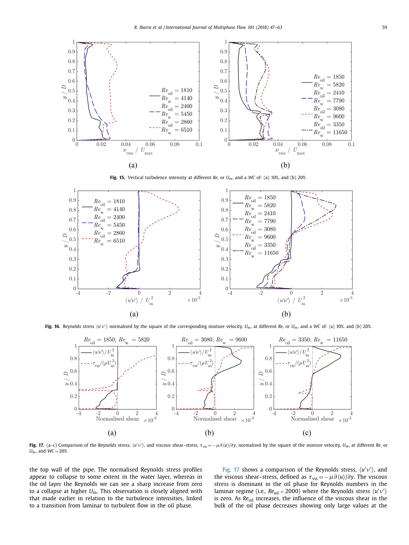
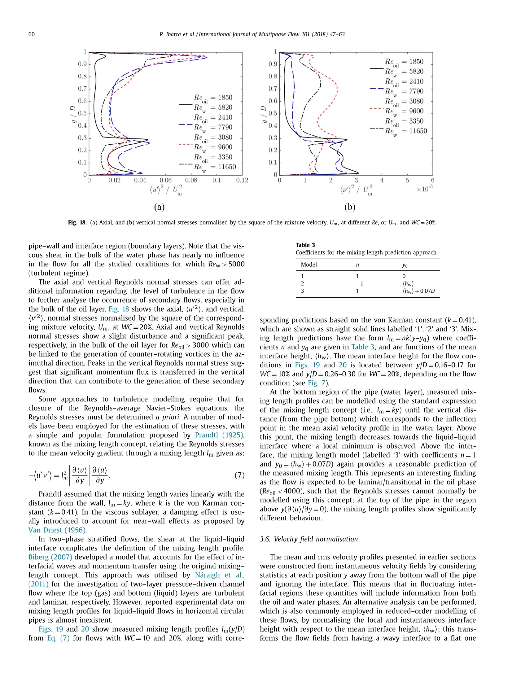
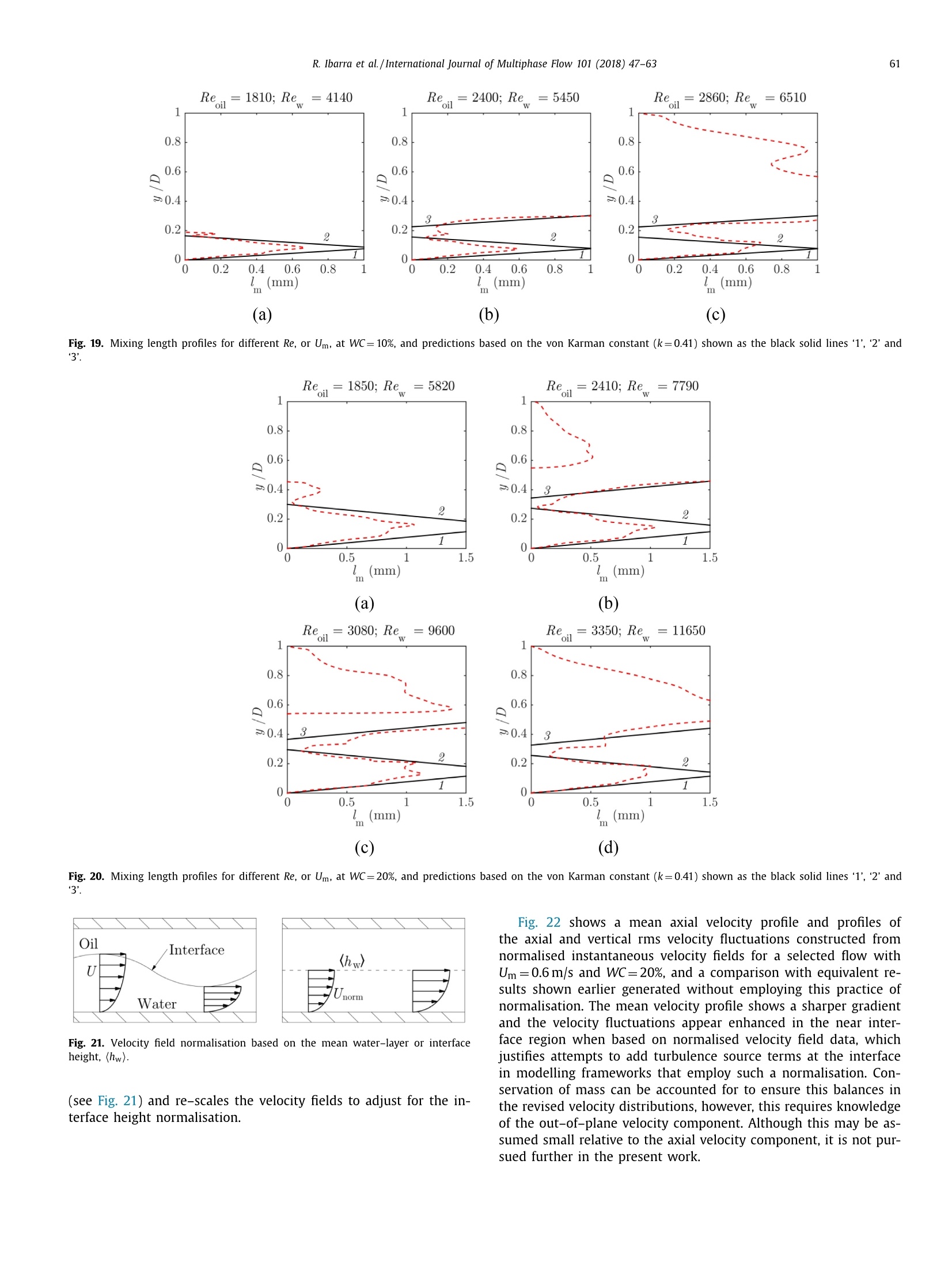
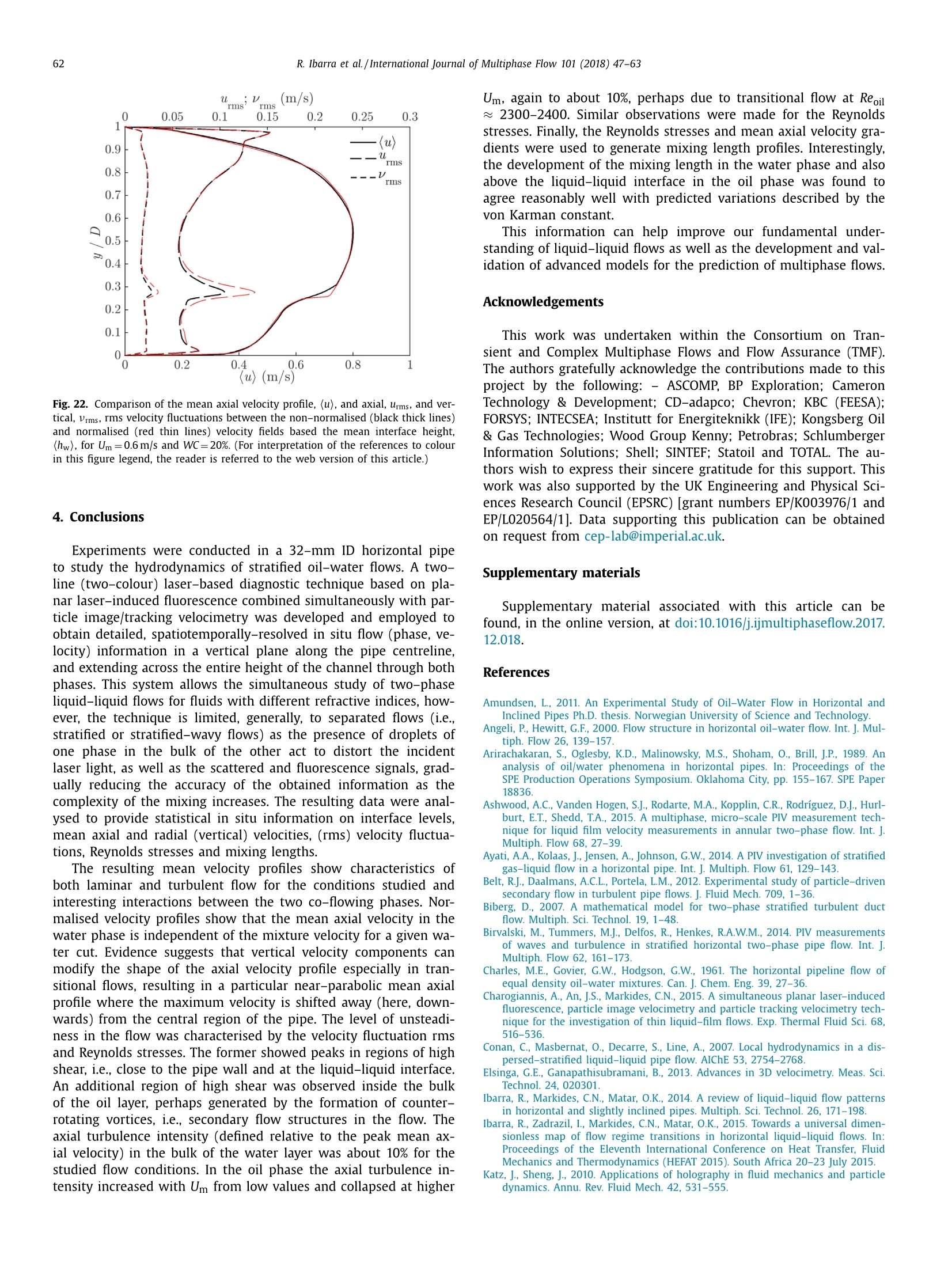
方案详情

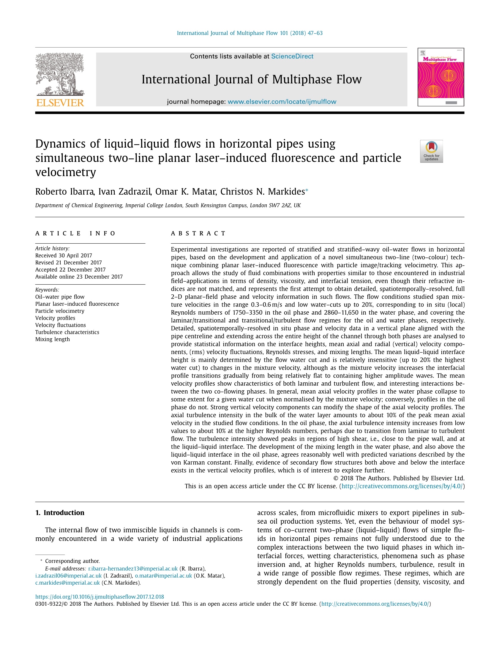
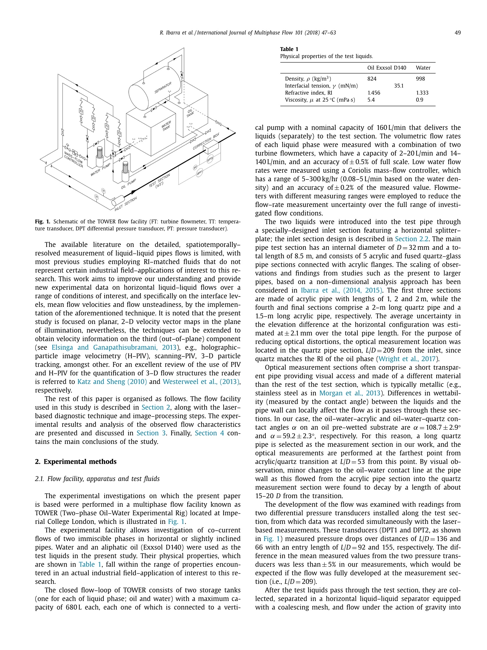
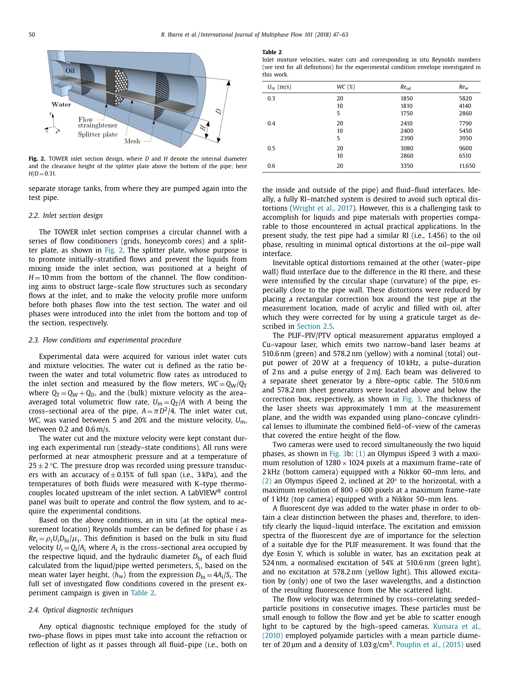
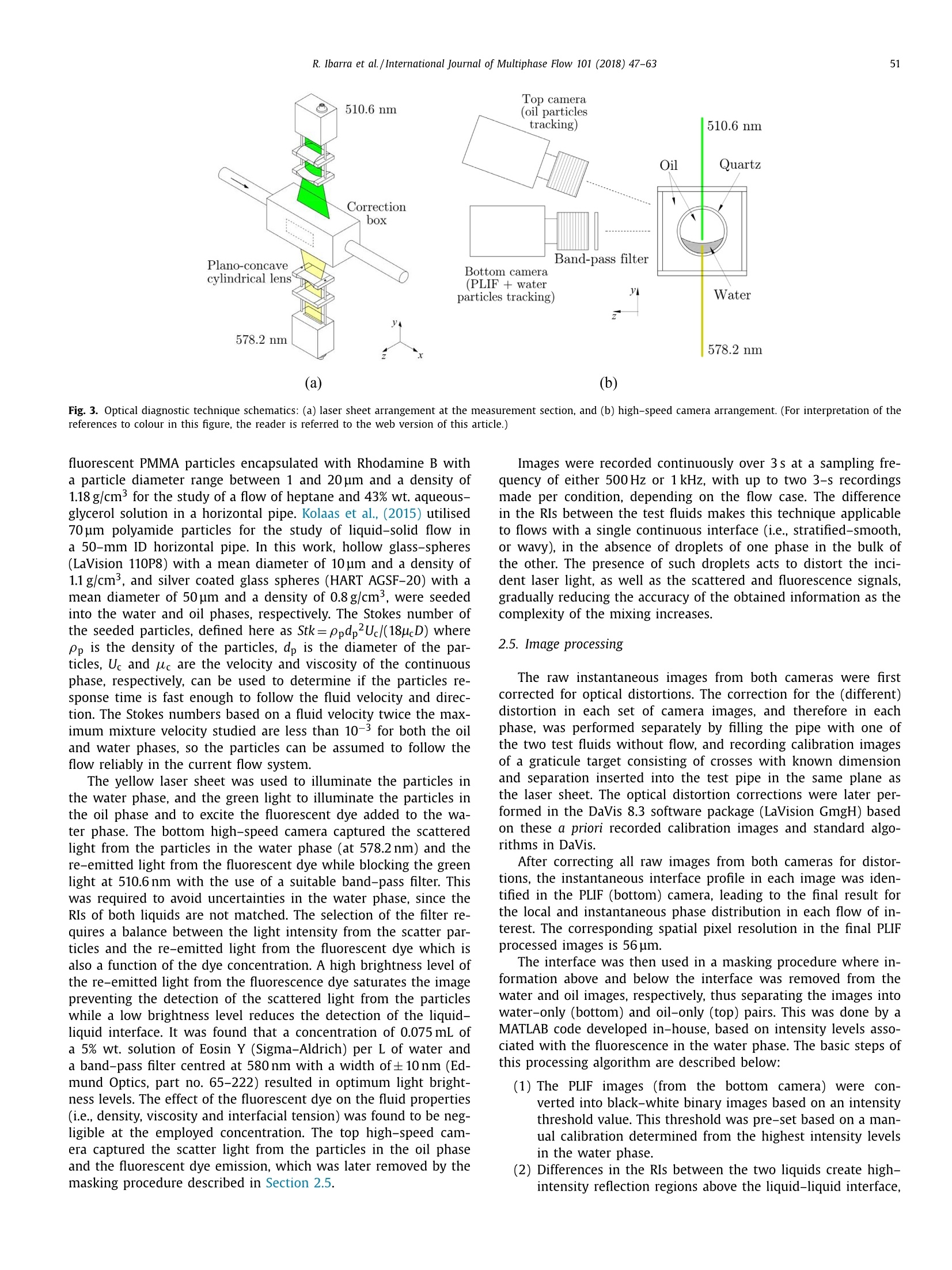
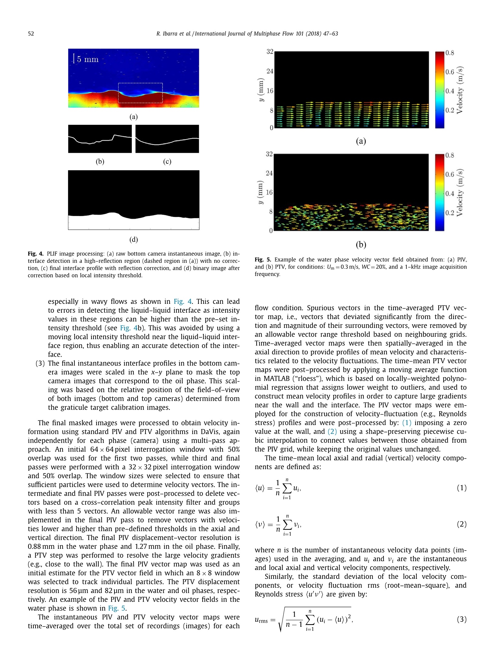
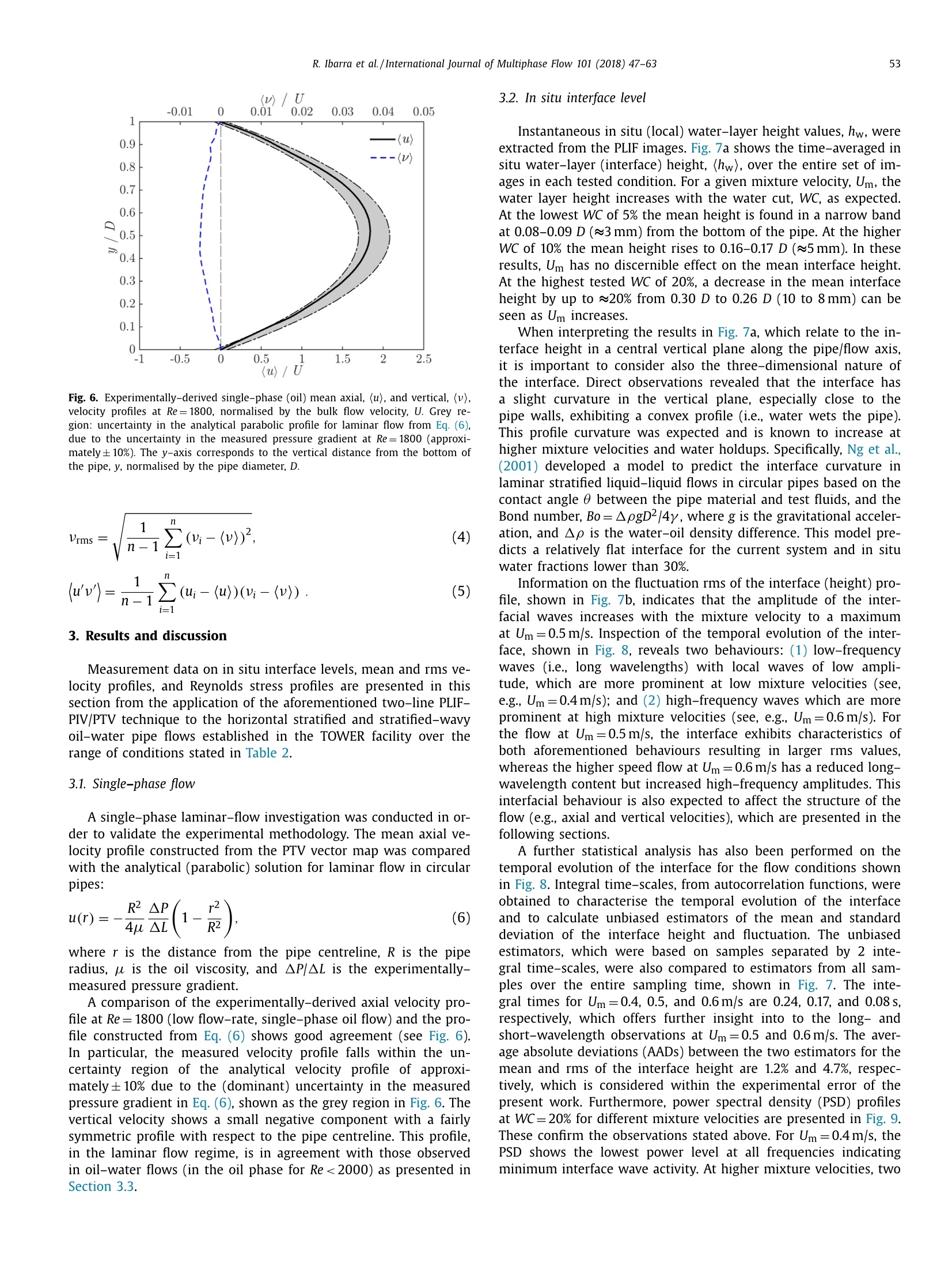
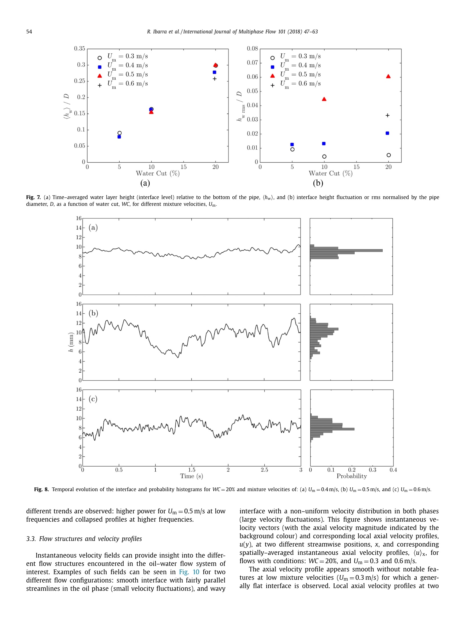
International Journal of Multiphase Flow 101 (2018) 47-63 0301-9322/O 2018 The Authors. Published by Elsevier Ltd. This is an open access article under the CC BY license. (http://creativecommons.org/licenses/by/4.0/) International Journal of Multiphase Flow ELSEVIER journal homepage: www.elsevier.com/locate/ijmulflow Dynamics of liquid-liquid flows in horizontal pipes usingsimultaneous two-line planar laser-induced fluorescence and particlevelocimetry Roberto Ibarra, Ivan Zadrazil, Omar K. Matar, Christos N. Markides* Department of Chemical Engineering, Imperial College London, South Kensington Campus, London SW7 2AZ, UK ABSTRACT Experimental investigations are reported of stratified and stratified-wavy oil-water flows in horizontalpipes, based on the development and application of a novel simultaneous two-line (two-colour) tech-nique combining planar laser-induced fluorescence with particle image/tracking velocimetry. This ap-proach allows the study of fluid combinations with properties similar to those encountered in industrialfield-applications in terms of density, viscosity, and interfacial tension, even though their refractive in-dices are not matched, and represents the first attempt to obtain detailed, spatiotemporally-resolved, full2-D planar-field phase and velocity information in such flows. The flow conditions studied span mix-ture velocities in the range 0.3-0.6 m/s and low water-cuts up to 20%, corresponding to in situ (local)Reynolds numbers of 1750-3350 in the oil phase and 2860-11,650 in the water phase, and covering thelaminar/transitional and transitional/turbulent flow regimes for the oil and water phases, respectively.Detailed, spatiotemporally-resolved in situ phase and velocity data in a vertical plane aligned with thepipe centreline and extending across the entire height of the channel through both phases are analysed toprovide statistical information on the interface heights, mean axial and radial (vertical) velocity compo-nents, (rms) velocity fluctuations, Reynolds stresses, and mixing lengths. The mean liquid-liquid interfaceheight is mainly determined by the flow water cut and is relatively insensitive (up to 20% the highestwater cut) to changes in the mixture velocity, although as the mixture velocity increases the interfacialprofile transitions gradually from being relatively flat to containing higher amplitude waves. The meanvelocity profiles show characteristics of both laminar and turbulent flow, and interesting interactions be-tween the two co-flowing phases. In general, mean axial velocity profiles in the water phase collapse tosome extent for a given water cut when normalised by the mixture velocity; conversely, profiles in the oilphase do not. Strong vertical velocity components can modify the shape of the axial velocity profiles. Theaxial turbulence intensity in the bulk of the water layer amounts to about 10% of the peak mean axialvelocity in the studied flow conditions. In the oil phase, the axial turbulence intensity increases from lowvalues to about 10% at the higher Reynolds numbers, perhaps due to transition from laminar to turbulentflow. The turbulence intensity showed peaks in regions of high shear, i.e., close to the pipe wall, and atthe liquid-liquid interface. The development of the mixing length in the water phase, and also above theliquid-liquid interface in the oil phase, agrees reasonably well with predicted variations described by thevon Karman constant. Finally, evidence of secondary flow structures both above and below the interfaceexists in the vertical velocity profiles, which is of interest to explore further. O 2018 The Authors. Published by Elsevier Ltd. 1. Introduction The internal flow of two immiscible liquids in channels is com-monly encountered in a wide variety of industrial applications ( * Corresponding author. ) E-mail addresses: r.ibarra-hernandez13@imperial.ac.uk(R. Ibarra), ( i.zadrazil06@imperial.ac.uk ( I . Zadrazil), o. m atar@impe r ia l .a c .u k (O .K. M a tar), c.mar k ides@impe r ial.ac.u k (C.N. Markides). ) across scales, from microfluidic mixers to export pipelines in sub-sea oil production systems. Yet, even the behaviour of model sys-tems of co-current two-phase (liquid-liquid) flows of simple flu-ids in horizontal pipes remains not fully understood due to thecomplex interactions between the two liquid phases in which in-terfacial forces, wetting characteristics, phenomena such as phaseinversion and, at higher Reynolds numbers,turbulence, result ina wide range of possible flow regimes. These regimes, which arestrongly dependent on the fluid properties (density, viscosity, and ( https://doi.org/10.1016/j.ijmultiphasef lo w.2017 . 12 . 0 18 ) interfacial tension), flow velocities, and pipe characteristics (diam-eter, inclination, roughness, and wettability), can be classified intotwo main categories: separated and mixed flows. Separated flowsare associated generally with the existence of two continuous fluidlayers on either side of a continuous interface that can be smoothor wavy, while mixed flows are more complex due to the appear-ance of droplets of one phase in the other (e.g., dual continuous,water-in-oil dispersions). Horizontal liquid-liquid flows have been studied by a numberof researchers, for example, Russell et al., (1959); Charles et al.,(1961); Arirachakaran et al., (1989); Trallero (1995); Soleimani(1999); Angeli and Hewitt (2000); and references therein. Themain purpose of these pioneering studies was to characterise theseflow in terms of flow-regime maps, pressure gradients and insitu phase fractions, which they achieved by employing a numberof intrusive and/or spatially-integrative and low-spatial-resolutionmeasurement techniques such as quick-closing valves, pressuretransducers, impedance probes, conductivity probes, and meshSensors. Further (e.g., velocity) information can be provided by hot-filmprobes, which make it possible to measure with excellent temporalresolution the time-varying velocity (mean and fluctuating compo-nents thereof) in liquid-liquid flows. However, the intrusive natureof this measurement can affect the flow in the region around theprobe, thereby modifying the flow such that it may not representthe conditions of the system under study, especially in flows withsignificant turbulence levels, and does not allow reliable measure-ments at or near the interface. The aforementioned techniques are not able to supply detailed,space- and time-resolved, full flow-field information, which is es-sential in promoting our understanding of these systems and forthe development of reliable predictive models. This has led to thedevelopment of non-intrusive measurement techniques, based onthe use of laser systems. The first laser-based technique used inthe extraction of local, in situ flow velocities was Laser DopplerAnemometry (LDA),employed by Yeh and Cummins (1964) to ob-tain velocity profiles in single-phase water flows. While this tech-nique offers high spatial resolution and fast dynamic response, andhas therefore proven to be an invaluable tool for the experimentalstudy of a wide range of flows, spatially-resolved information (i.e.,instantaneous velocity fields) cannot be obtained since it is a pointmeasurement generally limited to statistically-stationary or peri-odic flows if complete velocity profiles over the wall-normal coor-dinate are required (Morrison et al., 1994), and even then, a signif-icant amount of time is required to interrogate an entire flow field. Two-dimensional(2-D) spatiotemporal flow information can beobtained through the implementation of Planar-Laser Induced Flu-orescence (PLIF) and/or two- or three-dimensional Particle Imageor Tracking Velocimetry (PTV/PIV), which can also be applied si-multaneously. PLIF provides information on the scalar distributionof the two phases in the plane of the laser light, while PIV/PTVcan provide instantaneous velocity fields which are essential forobtaining profiles of mean velocity, turbulence intensity, Reynoldsstresses, as well as the strain rates at near-wall/near-interface re-gions. PLIF has been employed to characterise falling-film flowsover flat plates (Charogiannis et al., 2015; Markides et al., 2016),gas-liquid annular vertical flows (Schubring et al., 2010; Zadrazilet al., 2014), co-current liquid-liquid vertical downward pipe flows(Liu, 2005), and co-current liquid-liquid flows in horizontal pipes(Morgan et al., 2012;2013;2017). In PLIF, a horizontal flow is typ-ically illuminated by a thin laser light sheet passing through a ver-tical plane aligned with the pipe centreline.A distinction betweenthe phases is achieved by the addition of a fluorescent dye in oneof the phases. The fluorescent dye is excited by the laser light andemits spectrum-shifted light that is then captured by a high-speedcamera. In 2-D PIV/PTV, a laser light sheet is used to illuminate theflow (as in PLIF) and the Mie-scattered light from seeded par-ticles in the flow is captured by a high-speed camera. The po-sitions of the particles in instantaneous, successive image-pairsare cross-correlated to obtain displacement and, thus, velocitydata. In PIV, the cross-correlation is performed on particle groupswithin defined windows, while in PTV it is performed on in-dividual particles typically following PIV processing passes. PIVand PTV have been used to obtain velocity information in gas-liquid systems, e.g., by Zadrazil and Markides (2014) and alsoAshwood et al., (2015) who obtained velocity information insidethe liquid film in downward gas-liquid annular flow with differentapproaches, while Ayati et al., (2014) performed simultaneous PIVmeasurements in horizontal stratified air-water pipe flows, andBirvalski et al.,(2014) obtained measurements of velocity and wavecharacteristics in the liquid layer of gas-liquid stratified flows incircular horizontal pipes, in all cases supplying invaluable informa-tion on the flows of interest. The aforementioned optical techniques are associated with theirown set of challenges. In liquid-liquid systems, attempts have beenmade to match the refractive indices (RIs) of the test fluids for thepurpose of minimising light refraction or reflection at the interface.However, this often results in the selection of fluids with physicalproperties significantly different to those encountered in commonfield-applications, potentially leading to flows not entirely repre-sentative of actual industrial applications. In an excellent effort,Conan et al., (2007) performed experiments in dispersed-stratifiedflows in a 50-mm internal diameter horizontal acrylic pipe usingRI-matched fluids (i.e., heptane and a 50% vol. aqueous-glycerolsolution) to obtain detailed velocity and shear information nearthe wall and at the interface with PIV. Similarly, Morgan et al.,(2013)performed PLIF and PIV experiments in liquid-liquid flowsin a 25.4-mm internal diameter horizontal stainless-steel pipe(with a borosilicate glass measuring section) using the RI-matchedpair of Exxsol D80 and an 81.7% wt. aqueous-glycerol solution,which also matched the RI of the borosilicate measuring section,thus further minimising optical distortions. Simultaneous informa-tion in both phases was obtained using a single laser-sheet; how-ever, the viscosity of the resulting glycerol solution was approxi-mately 43 times higher than that of the oil phase, which is notcommonly observed in industrial applications with the exceptionof oil-water systems with ethylene glycol used to prevent the for-mation of hydrates. Inanother particularly interesting effort,Kumaraet al(2010) employed PIV to characterise the flow structures in oil-water flow in a 56-mm diameter stainless steel pipe. The RIs ofthe test fluids were not matched, hence, the light was refractedas it passed through the liquid-liquid interface enabling accurateinformation to be obtained in only one phase (i.e.,before the lightreached the interface). The experimental procedure was carried outin two steps: firstly, the flow was illuminated with the laser sheetfrom top to bottom to obtain information in the (top) oil phase;secondly, the laser sheet was introduced from the bottom of thepipe to obtain information in the water phase. This proved to be avery worthy effort in terms of supplying statistical information inthe two liquid phases, but even so, in some cases, it is of interestto generate simultaneous information in both phases. The need for this type of information motivated the develop-ment of a simultaneous planar combined LIF and PIV/PTV tech-nique in the present work, which employs a second laser-sheet ata different wavelength, and its application to the horizontal liquid-liquid flows of interest that feature two test fluids with differ-ent RIs. To the best of the authors' knowledge, the present workrepresents the first attempt to obtain detailed, spatiotemporally-resolved, full planar-field phase and 2-D velocity information insuch flows of selected fluids with mismatched RIs. Fig. 1. Schematic of the TOWER flow facility (FT: turbine flowmeter, TT: tempera-ture transducer, DPT differential pressure transducer, PT: pressure transducer). The available literature on the detailed, spatiotemporally-resolved measurement of liquid-liquid pipes flows is limited, withmost previous studies employing RI-matched fluids that do notrepresent certain industrial field-applications of interest to this re-search. This work aims to improve our understanding and providenew experimental data on horizontal liquid-liquid flows over arange of conditions of interest, and specifically on the interface lev-els, mean flow velocities and flow unsteadiness, by the implemen-tation of the aforementioned technique. It is noted that the presentstudy is focused on planar, 2-D velocity vector maps in the planeof illumination, nevertheless, the techniques can be extended toobtain velocity information on the third (out-of-plane) component(see Elsinga and Ganapathisubramani, 2013), e.g., holographic-particle image velocimetry (H-PIV), scanning-PIV, 3-D particletracking, amongst other. For an excellent review of the use of PIVand H-PIV for the quantification of 3-D flow structures the readeris referred to Katz and Sheng (2010) and Westerweel et al., (2013),respectively. The rest of this paper is organised as follows. The flow facilityused in this study is described in Section 2, along with the laser-based diagnostic technique and image-processing steps. The exper-imental results and analysis of the observed flow characteristicsare presented and discussed in Section 3. Finally, Section 4 con-tains the main conclusions of the study. 2. Experimental methods 2.1. Flow facility, apparatus and test fluids The experimental investigations on which the present paperis based were performed in a multiphase flow facility known asTOWER (Two-phase Oil-Water Experimental Rig) located at Impe-rial College London, which is illustrated in Fig. 1. The experimental facility allows investigation of co-currentflows of two immiscible phases in horizontal or slightly inclinedpipes. Water and an aliphatic oil (Exxsol D140) were used as thetest liquids in the present study. Their physical properties, whichare shown in Table 1, fall within the range of properties encoun-tered in an actual industrial field-application of interest to this re-Search. The closed flow-loop of TOWER consists of two storage tanks(one for each of liquid phase; oil and water) with a maximum ca-pacity of 680L each, each one of which is connected to a verti- Oil Exxsol D140 Water Density, p (kg/m’) 824 35.1 998 Interfacial tension, y (mN/m) Refractive index, RI 1.456 1.333 Viscosity, p at 25℃ (mPas) 5.4 0.9 cal pump with a nominal capacity of 160L/min that delivers theliquids (separately) to the test section. The volumetric flow ratesof each liquid phase were measured with a combination of twoturbine flowmeters, which have a capacity of 2-20L/min and 14-140 L/min, and an accuracy of±0.5% of full scale. Low water flowrates were measured using a Coriolis mass-flow controller, whichhas a range of 5-300kg/hr (0.08-5L/min based on the water den-sity) and an accuracy of±0.2% of the measured value. Flowme-ters with different measuring ranges were employed to reduce theflow-rate measurement uncertainty over the full range of investi-gated flow conditions. The two liquids were introduced into the test pipe througha specially-designed inlet section featuring a horizontal splitter-plate; the inlet section design is described in Section 2.2. The mainpipe test section has an internal diameter of D=32 mm and a to-tal length of 8.5 m, and consists of 5 acrylic and fused quartz-glasspipe sections connected with acrylic flanges. The scaling of obser-vations and findings from studies such as the present to largerpipes, based on a non-dimensional analysis approach has beenconsidered in Ibarra et al., (2014, 2015). The first three sectionsare made of acrylic pipe with lengths of 1, 2 and 2 m, while thefourth and final sections comprise a 2-m long quartz pipe and a1.5-m long acrylic pipe, respectively. The average uncertainty inthe elevation difference at the horizontal configuration was esti-mated at±2.1 mm over the total pipe length. For the purpose ofreducing optical distortions, the optical measurement location waslocated in the quartz pipe section, L/D=209 from the inlet, sincequartz matches the RI of the oil phase (Wright et al., 2017). Optical measurement sections often comprise a short transpar-ent pipe providing visual access and made of a different materialthan the rest of the test section, which is typically metallic (e.g.,stainless steel as in Morgan et al., 2013). Differences in wettabil-ity (measured by the contact angle) between the liquids and thepipe wall can locally affect the flow as it passes through these sec-tions. In our case, the oil-water-acrylic and oil-water-quartz con-tact angles a on an oil pre-wetted substrate are α=108.7±2.9°and α=59.2±2.3°, respectively. For this reason, a long quartzpipe is selected as the measurement section in our work, and theoptical measurements are performed at the farthest point fromacrylic/quartz transition at L|D=53 from this point. By visual ob-servation, minor changes to the oil-water contact line at the pipewall as this flowed from the acrylic pipe section into the quartzmeasurement section were found to decay by a length of about15-20 D from the transition. The development of the flow was examined with readings fromtwo differential pressure transducers installed along the test sec-tion, from which data was recorded simultaneously with the laser-based measurements. These transducers (DPT1 and DPT2, as shownin Fig. 1) measured pressure drops over distances of L/D=136 and66 with an entry length of L/D=92 and 155, respectively. The dif-ference in the mean measured values from the two pressure trans-ducers was less than±5% in our measurements,which would beexpected if the flow was fully developed at the measurement sec-tion (i.e., L/D=209). After the test liquids pass through the test section, they are col-lected, separated in a horizontal liquid-liquid separator equippedwith a coalescing mesh, and flow under the action of gravity into Fig. 2. TOWER inlet section design, where D and H denote the internal diameterand the clearance height of the splitter plate above the bottom of the pipe; hereH|D=0.31. separate storage tanks, from where they are pumped again into thetest pipe. 2.2. Inlet section design The TOWER inlet section comprises a circular channel with aseries of flow conditioners (grids, honeycomb cores) and a split-ter plate, as shown in Fig. 2. The splitter plate, whose purpose isto promote initially-stratified flows and prevent the liquids frommixing inside the inlet section, was positioned at a height ofH=10mm from the bottom of the channel. The flow condition-ing aims to obstruct large-scale flow structures such as secondaryflows at the inlet, and to make the velocity profile more uniformbefore both phases flow into the test section. The water and oilphases were introduced into the inlet from the bottom and top ofthe section, respectively. 2.3. Flow conditions and experimental procedure Experimental data were acquired for various inlet water cutsand mixture velocities. The water cut is defined as the ratio be-tween the water and total volumetric flow rates as introduced tothe inlet section and measured by the flow meters, WC=Qw/Qrwhere Qr=Qw+Qo, and the (bulk) mixture velocity as the area-averaged total volumetric flow rate, Um=QT/A with A being thecross-sectional area of the pipe, A=nD/4. The inlet water cut,WC, was varied between 5 and 20% and the mixture velocity, Um,between 0.2 and 0.6 m/s. The water cut and the mixture velocity were kept constant dur-ing each experimental run (steady-state conditions). All runs wereperformed at near atmospheric pressure and at a temperature of25±2°C. The pressure drop was recorded using pressure transduc-ers with an accuracy of±0.15% of full span (i.e.,3kPa), and thetemperatures of both fluids were measured with K-type thermo-couples located upstream of the inlet section. A LabVIEW@ controlpanel was built to operate and control the flow system, and to ac-quire the experimental conditions. 2.4. Optical diagnostic techniques Any optical diagnostic technique employed for the study oftwo-phase flows in pipes must take into account the refraction orreflection of light as it passes through all fluid-pipe (i.e., both on Inlet mixture velocities, water cuts and corresponding in situ Reynolds numbers(see text for all definitions) for the experimental condition envelope investigated inthis work. Um (m/s) WC(%) Reoil Rew 0.3 20 1850 5820 10 1810 4140 5 1750 2860 0.4 20 2410 7790 10 2400 5450 5 2390 3950 0.5 20 3080 9600 10 2860 6510 0.6 20 3350 11.650 the inside and outside of the pipe) and fluid-fluid interfaces. Ide-ally, a fully RI-matched system is desired to avoid such optical dis-tortions (Wright et al., 2017). However, this is a challenging task toaccomplish for liquids and pipe materials with properties compa-rable to those encountered in actual practical applications. In thepresent study, the test pipe had a similar RI (i.e., 1.456) to the oilphase, resulting in minimal optical distortions at the oil-pipe wallinterface. Inevitable optical distortions remained at the other (water-pipewall) fluid interface due to the difference in the RI there, and thesewere intensified by the circular shape (curvature) of the pipe, es-pecially close to the pipe wall. These distortions were reduced byplacing a rectangular correction box around the test pipe at themeasurement location, made of acrylic and filled with oil, afterwhich they were corrected for by using a graticule target as de-scribed in Section 2.5. The PLIF-PIV/PTV optical measurement apparatus employed aCu-vapour laser, which emits two narrow-band laser beams at510.6 nm (green) and 578.2 nm (yellow) with a nominal (total) out-put power of 20W at a frequency of 10kHz, a pulse-durationof 2ns and a pulse energy of 2 mJ. Each beam was delivered toa separate sheet generator by a fibre-optic cable. The 510.6 nmand 578.2 nm sheet generators were located above and below thecorrection box, respectively, as shown in Fig. 3. The thickness ofthe laser sheets was approximately 1mm at the measurementplane, and the width was expanded using plano-concave cylindri-cal lenses to illuminate the combined field-of-view of the camerasthat covered the entire height of the flow. Two cameras were used to record simultaneously the two liquidphases, as shown in Fig. 3b:(1) an Olympus iSpeed 3 with a maxi-mum resolution of 1280 ×1024 pixels at a maximum frame-rate of2 kHz (bottom camera) equipped with a Nikkor 60-mmlens, and(2) an Olympus iSpeed 2, inclined at 20° to the horizontal, with amaximum resolution of 800×600 pixels at a maximum frame-rateof 1 kHz (top camera) equipped with a Nikkor 50-mm lens. A fluorescent dye was added to the water phase in order to ob-tain a clear distinction between the phases and, therefore, to iden-tify clearly the liquid-liquid interface. The excitation and emissionspectra of the fluorescent dye are of importance for the selectionof a suitable dye for the PLIF measurement. It was found that thedye Eosin Y, which is soluble in water, has an excitation peak at524 nm, a normalised excitation of 54% at 510.6nm (green light),and no excitation at 578.2 nm (yellow light). This allowed excita-tion by (only) one of two the laser wavelengths, and a distinctionof the resulting fluorescence from the Mie scattered light. The flow velocity was determined by cross-correlating seeded-particle positions in consecutive images. These particles must besmall enough to follow the flow and yet be able to scatter enoughlight to be captured by the high-speed cameras. Kumara et al.,(2010) employed polyamide particles with a mean particle diame-ter of 20 um and a density of 1.03 g/cm3. Pouplin et al., (2015) used x (a) (b) Fig. 3. Optical diagnostic technique schematics: (a) laser sheet arrangement at the measurement section, and (b) high-speed camera arrangement. (For interpretation of thereferences to colour in this figure, the reader is referred to the web version of this article.) fluorescent PMMA particles encapsulated with Rhodamine B witha particle diameter range between 1 and 20um and a density of1.18 g/cm3 for the study of a flow of heptane and 43% wt. aqueous-glycerol solution in a horizontal pipe. Kolaas et al., (2015) utilised70 um polyamide particles for the study of liquid-solid flow ina 50-mm ID horizontal pipe. In this work, hollow glass-spheres(LaVision 110P8) with a mean diameter of 10 um and a density of1.1 g/cm3, and silver coated glass spheres (HART AGSF-20) with amean diameter of 50um and a density of 0.8g/cm3, were seededinto the water and oil phases, respectively. The Stokes number ofthe seeded particles, defined here as Stk=ppdp2Uc/(18ucD) wherepp is the density of the particles, dp is the diameter of the par-ticles, Ue and pc are the velocity and viscosity of the continuousphase, respectively, can be used to determine if the particles re-sponse time is fast enough to follow the fluid velocity and direc-tion. The Stokes numbers based on a fluid velocity twice the max-imum mixture velocity studied are less than 10-3 for both the oiland water phases, so the particles can be assumed to follow theflow reliably in the current flow system. The yellow laser sheet was used to illuminate the particles inthe water phase, and the green light to illuminate the particles inthe oil phase and to excite the fluorescent dye added to the wa-ter phase. The bottom high-speed camera captured the scatteredlight from the particles in the water phase (at 578.2 nm) and there-emitted light from the fluorescent dye while blocking the greenlight at 510.6nm with the use of a suitable band-pass filter. Thiswas required to avoid uncertainties in the water phase, since theRIs of both liquids are not matched. The selection of the filter re-quires a balance between the light intensity from the scatter par-ticles and the re-emitted light from the fluorescent dye which isalso a function of the dye concentration. A high brightness level ofthe re-emitted light from the fluorescence dye saturates the imagepreventing the detection of the scattered light from the particleswhile a low brightness level reduces the detection of the liquid-liquid interface. It was found that a concentration of 0.075 mL ofa 5% wt. solution of Eosin Y (Sigma-Aldrich) per L of water anda band-pass filter centred at 580 nm with a width of±10 nm (Ed-mund Optics, part no. 65-222) resulted in optimum light bright-ness levels. The effect of the fluorescent dye on the fluid properties(i.e., density, viscosity and interfacial tension) was found to be neg-ligible at the employed concentration. The top high-speed cam-era captured the scatter light from the particles in the oil phaseand the fluorescent dye emission, which was later removed by themasking procedure described in Section 2.5. Images were recorded continuously over 3s at a sampling fre-quency of either 500 Hz or 1 kHz, with up to two 3-s recordingsmade per condition, depending on the flow case. The differencein the RIs between the test fluids makes this technique applicableto flows with a single continuous interface (i.e., stratified-smooth,or wavy), in the absence of droplets of one phase in the bulk ofthe other. The presence of such droplets acts to distort the inci-dent laser light, as well as the scattered and fluorescence signalsgradually reducing the accuracy of the obtained information as thecomplexity of the mixing increases. 2.5. Image processing The raw instantaneous images from both cameras were firstcorrected for optical distortions. The correction for the (different)distortion in each set of camera images, and therefore in eachphase, was performed separately by filling the pipe with one ofthe two test fluids without flow, and recording calibration imagesof a graticule target consisting of crosses with known dimensionand separation inserted into the test pipe in the same plane asthe laser sheet. The optical distortion corrections were later per-formed in the DaVis 8.3 software package (LaVision GmgH) basedon these a priori recorded calibration images and standard algo-rithms in DaVis. After correcting all raw images from both cameras for distor-tions, the instantaneous interface profile in each image was iden-tified in the PLIF (bottom) camera, leading to the final result forthe local and instantaneous phase distribution in each flow of in-terest. The corresponding spatial pixel resolution in the final PLIFprocessed images is 56um. The interface was then used in a masking procedure where in-formation above and below the interface was removed from thewater and oil images, respectively, thus separating the images intowater-only (bottom) and oil-only(top) pairs. This was done by aMATLAB code developed in-house, based on intensity levels asso-ciated with the fluorescence in the water phase. The basic steps ofthis processing algorithm are described below: (1) The PLIF images (from the bottom camera)l) were con-verted into black-white binary images based on an intensitythreshold value. This threshold was pre-set based on a man-ual calibration determined from the highest intensity levelsin the water phase. (2) Differences in the RIs between the two liquids create high-intensity reflection regions above the liquid-liquid interface, (d) Fig. 4. PLIF image processing: (a) raw bottom camera instantaneous image, (b) in-terface detection in a high-reflection region (dashed region in (a)) with no correc-tion, (c) final interface profile with reflection correction, and (d) binary image aftercorrection based on local intensity threshold. especially in wavy flows as shown in Fig. 4. This can leadto errors in detecting the liquid-liquid interface as intensityvalues in these regions can be higher than the pre-set in-tensity threshold (see Fig. 4b). This was avoided by using amoving local intensity threshold near the liquid-liquid inter-face region, thus enabling an accurate detection of the inter-face. (3) The final instantaneous interface profiles in the bottom cam-era images were scaled in the x-y plane to mask the topcamera images that correspond to the oil phase. This scal-ing was based on the relative position of the field-of-viewof both images (bottom and top cameras) determined fromthe graticule target calibration images. The instantaneous PIV and PTV velocity vector maps weretime-averaged over the total set of recordings (images) for each (a) (b) Fig. 5. Example of the water phase velocity vector field obtained from: (a) PIV,Weand (b) PTV, for conditions: Um=0.3 m/s, WC=20%, and a 1-kHz image acquisitionfrequency. flow condition. Spurious vectors in the time-averaged PTV vec-tor map, i.e., vectors that deviated significantly from the direc-tion and magnitude of their surrounding vectors, were removed byan allowable vector range threshold based on neighbouring grids.Time-averaged vector maps were then spatially-averaged in theaxial direction to provide profiles of mean velocity and characteris-tics related to the velocity fluctuations. The time-mean PTV vectormaps were post-processed by applying a moving average functionin MATLAB (“rloess"), which is based on locally-weighted polyno-mial regression that assigns lower weight to outliers, and used toconstruct mean velocity profiles in order to capture large gradientsnear the wall and the interface. The PIV vector maps were em-ployed for the construction of velocity-fluctuation (e.g., Reynoldsstress) profiles and were post-processed by: (1) imposing a zerovalue at the wall, and (2) using a shape-preserving piecewise cu-bic interpolation to connect values between those obtained fromthe PIV grid, while keeping the original values unchanged. The time-mean local axial and radial (vertical) velocity compo-nents are defined as: where n is the number of instantaneous velocity data points (im-ages) used in the averaging, and uj and vi are the instantaneousand local axial and vertical velocity components, respectively. Similarly, the standard deviation of the local velocity com-ponents, or velocity fluctuation rms (root-mean-square), andReynolds stress (u’v’) are given by: Fig. 6. Experimentally-derived single-phase (oil) mean axial, (u), and vertical, (v),velocity profiles at Re=1800, normalised by the bulk flow velocity, U. Grey re-gion: uncertainty in the analytical parabolic profile for laminar flow from Eq. (6),due to the uncertainty in the measured pressure gradient at Re=1800 (approxi-mately±10%). The y-axis corresponds to the vertical distance from the bottom ofthe pipe, y, normalised by the pipe diameter, D. 3. Results and discussion Measurement data on in situ interface levels, mean and rms ve-locity profiles, and Reynolds stress profiles are presented in thissection from the application of the aforementioned two-line PLIF-PIV/PTV technique to the horizontal stratified and stratified-wavyoil-water pipe flows established in the TOWER facility over therange of conditions stated in Table 2. 3.1. Single-phase flow A single-phase laminar-flow investigation was conducted in or-der to validate the experimental methodology. The mean axial ve-locity profile constructed from the PTV vector map was comparedwith the analytical (parabolic) solution for laminar flow in circularpipes: where r is the distance from the pipe centreline, R is the piperadius, u is the oil viscosity, and AP/AL is the experimentally-measured pressure gradient. A comparison of the experimentally-derived axial velocity pro-file at Re=1800 (low flow-rate, single-phase oil flow) and the pro-file constructed from Eq. (6) shows good agreement (see Fig. 6).In particular, the measured velocity profile falls within the un-certainty region of the analytical velocity profile of approxi-mately±10% due to the (dominant) uncertainty in the measuredpressure gradient in Eq. (6), shown as the grey region in Fig. 6. Thevertical velocity shows a small negative component with a fairlysymmetric profile with respect to the pipe centreline. This profile,in the laminar flow regime, is in agreement with those observedin oil-water flows (in the oil phase for Re<2000) as presented inSection 3.3. Instantaneous in situ (local) water-layer height values, hw, wereextracted from the PLIF images. Fig. 7a shows the time-averaged insitu water-layer (interface) height, (hw), over the entire set of im-ages in each tested condition. For a given mixture velocity, Um, thewater layer height increases with the water cut, WC, as expected.At the lowest WC of 5% the mean height is found in a narrow bandat 0.08-0.09 D (~3 mm) from the bottom of the pipe. At the higherWC of 10% the mean height rises to 0.16-0.17 D (~5mm). In theseresults, Um has no discernible effect on the mean interface heightAt the highest tested WC of 20%, a decrease in the mean interfaceheight by up to ~20% from 0.30 D to 0.26 D (10 to 8 mm) can beseen as Um increases. When interpreting the results in Fig. 7a, which relate to the in-terface height in a central vertical plane along the pipe/flow axis,it is important to consider also the three-dimensional nature ofthe interface. Direct observations revealed that the interface hasa slight curvature in the vertical plane, especially close to thepipe walls, exhibiting a convex profile (i.e., water wets the pipe).This profile curvature was expected and is known to increase athigher mixture velocities and water holdups. Specifically, Ng et al.,(2001) developed a model to predict the interface curvature inlaminar stratified liquid-liquid flows in circular pipes based on thecontact angle 0 between the pipe material and test fluids, and theBond number, Bo=△pgD2/4y, where g is the gravitational acceler-ation, and Ap is the water-oil density difference. This model predicts a relatively flat interface for the current system and in situwater fractions lower than 30%. Information on the fluctuation rms of the interface (height) pro-file, shown in Fig. 7b, indicates that the amplitude of the inter-facial waves increases with the mixture velocity to a maximumat Um=0.5 m/s. Inspection of the temporal evolution of the inter-face, shown in Fig. 8, reveals two behaviours: (1) low-frequencywaves (i.e., long wavelengths) with local waves of low ampli-tude, which are more prominent at low mixture velocities (see,e.g., Um=0.4m/s); and (2) high-frequency waves which are moreprominent at high mixture velocities (see, e.g., Um=0.6 m/s). Forthe flow at Um=0.5 m/s, the interface exhibits characteristics ofboth aforementioned behaviours resulting in larger rms values,whereas the higher speed flow at Um=0.6 m/s has a reduced long-wavelength content but increased high-frequency amplitudes. Thisinterfacial behaviour is also expected to affect the structure of theflow (e.g., axial and vertical velocities), which are presented in thefollowing sections. A further statistical analysis has also been performed on thetemporal evolution of the interface for the flow conditions shownin Fig. 8. Integral time-scales, from autocorrelation functions, wereobtained to characterise the temporal evolution of the interfaceand to calculate unbiased estimators of the mean and standarddeviation of the interface height and fluctuation. The unbiasedestimators, which were based on samples separated by 2 inte-gral time-scales, were also compared to estimators from all sam-ples over the entire sampling time, shown in Fig. 7. The inte-gral times for Um=0.4, 0.5, and 0.6 m/s are 0.24, 0.17, and 0.08 s,respectively, which offers further insight into to the long- andshort-wavelength observations at Um=0.5 and 0.6 m/s. The aver-age absolute deviations (AADs) between the two estimators for themean and rms of the interface height are 1.2% and 4.7%, respec-tively, which is considered within the experimental error of thepresent work. Furthermore, power spectral density (PSD) profilesat WC=20% for different mixture velocities are presented in Fig. 9.These confirm the observations stated above. For Um=0.4 m/s, thePSD shows the lowest power level at all frequencies indicatingminimum interface wave activity. At higher mixture velocities, two (a) (b) Fig.7. (a) Time-averaged water layer height (interface level) relative to the bottom of the pipe, (hw), and (b) interface height fluctuation or rms normalised by the pipediameter, D, as a function of water cut, WC, for different mixture velocities, Um. Fig. 8. Temporal evolution of the interface and probability histograms for WC=20% and mixture velocities of: (a) Um=0.4 m/s, (b) Um=0.5 m/s, and (c) Um=0.6m/s. different trends are observed: higher power for Um=0.5 m/s at lowfrequencies and collapsed profiles at higher frequencies. 3.3. Flow structures and velocity profiles Instantaneous velocity fields can provide insight into the differ-ent flow structures encountered in the oil-water flow system ofinterest. Examples of such fields can be seen in Fig. 10 for twodifferent flow configurations: smooth interface with fairly parallelstreamlines in the oil phase (small velocity fluctuations), and wavy interface with a non-uniform velocity distribution in both phases(large velocity fluctuations). This figure shows instantaneous ve-locity vectors (with the axial velocity magnitude indicated by thebackground colour) and corresponding local axial velocity profiles,u(y), at two different streamwise positions, x, and correspondingspatially-averaged instantaneous axial velocity profiles, (u)x, forflows with conditions: WC=20%, and Um=0.3 and 0.6 m/s. The axial velocity profile appears smooth without notable fea-tures at low mixture velocities (Um=0.3 m/s) for which a gener-ally flat interface is observed. Local axial velocity profiles at two Fig. 9. Interface temporal evolution PSD for different mixture velocities, Um, andWC=20%. different streamwise positions show very similar profiles, espe-cially in the oil layer, resulting in low velocity fluctuation rms val-ues (shown as the error bar in the spatially-averaged instanta-neous axial velocity profiles, (u)x) in the oil layer. With increasingUm, and therefore Reoil and Rew, more complex velocity structuresgradually appear in the flow field, as the axial velocity profiles be-gin to show unsteadiness resulting in an increase in the velocity fluctuations. This is also observed in the rms velocity fluctuationprofiles discussed in the next section. Mean (time-averaged) axial velocity profiles,(u), and mean ver-tical velocity profiles, (v), have been normalised by their respec-tive mixture velocities, Um, to identify common trends for differentflow conditions. Fig. 11 shows the normalised (u)/Um and (v)Umprofiles for water cuts in the range WC=5-20% at a mixture veloc-ity of Um =0.3 m/s. The mean axial profiles reflect laminar flow be-haviour in the oil phase and transitional/turbulent flow behaviourin the water phase. This is consistent with expectations from thein situ Reynolds number values given in Table 2 for these flows,although it is noted that this only provides an approximate indi-cation based on single-phase pipe flows which, generally, can ex-hibit turbulence characteristics for Reynolds numbers above 2000.In two-phase flow systems, the flow is destabilised by the pres-ence of an interface, with unstable ‘interfacial modes’appearingdue to viscosity-stratification at arbitrary small Reynolds numbers(Yih, 1967; Yiantsios and Higgins, 1988; Naraigh et al., 2011). The normalised mean axial velocity profiles collapse in the oilphase, with the exception of the profile associated with the lowestwater cut, WC=5%. The normalised mean vertical velocity profilesshow negative values in the oil phase for the cases studied, mean-ing that the oil phase flows towards the interface, with a verticalof velocity component that appears to be relatively uniform overy/D and a pronounced peak at the interface in the WC=20% flowcase. Similarly, the water phase flows towards the bottom of thepipe, except for the WC=5% flow case, for which there is a near-zero vertical flow component. These observations indicate that sec- 0.2z (mm)(a) 32 32 (b) Fig. 10. Instantaneous velocity fields (the axial velocity magnitude is indicated by the colour-plot, and the interface profile by the black solid line), with corresponding localaxial velocity profiles,u(y), and spatially-averaged axial velocity profiles,(u)x(y), for WC=20% and mixture velocities of: (a) Um=0.3m/s (Reoil=1850, Rew=5820), and (b)Um=0.6m/s (Reoil=3350, Rew=11,650). The vertical distance, y, is measured from the bottom of the pipe. The error bars in the (u)x profiles indicate the local axial velocity111rms, not the experimental error (for ease of visualisation not all vectors are shown in the velocity fields). (a) (b) Fig. 11. Normalised mean: (a) axial velocity profiles, and (b) vertical velocity profiles, at different water cuts for Um=0.3m/s (Reoil=1750, Rew=2860 for WC=5%;Reoil=1810, Rew=4140 for WC=10%; Reoil=1850, Rew=5820 for WC=20%). The in situ interface positions for all flows can be found in Fig. 7, and these generally matchthe velocity gradient discontinuities at y/D≈0.08-0.09, 0.16-0.17, 0.26-0.30 for WC=5, 10, 20%, respectively. ondary flows are present in the system, as will be described inSection 3.4. It is expected that increased vertical velocity gradients will actto transfer momentum over the flow section, and that this willmanifest itself in the shapes of the various profiles. Consider Fig. 12for Um=0.4 m/s. In Fig. 12a, the mean axial velocity profiles in theoil phase for WC=5% and 10% have a maximum at a location thathas been shifted from the central region of the pipe to a region justabove the liquid-liquid interface. This is at odds with the shape ofthe mean axial velocity profile observed at the other flow condi-tion (WC=20%), where the maximum velocity is encountered nearthe centre of the pipe. This can be considered in light of the corre-sponding mean vertical velocity profiles in Fig. 12c, which indicatefaster oil flows towards the interface for WC=5 and 10% in com-parison to WC=20% and suggest that significant vertical momen-tum is transferred downwards, and towards the interface region. From inspection of Fig. 12d, which includes all flow cases withWC=10%, we see that for the lower-speed flows (Um ≤ 0.4 m/s) inthe laminar/transitional regimes (Reoil≤2400), the mean verticalvelocity component shows negative values in the oil phase, whichtherefore flows downward towards the interface. Above this veloc-ity (Um=0.5 m/s, Rei=2860), the flow reverses and moves up-ward in the core region the oil phase. This behaviour has not beenobserved in previous studies, which have generally considered flowconditions with Reynolds numbers either in the fully laminar orfully turbulent regimes (e.g., Kumara et al., 2010; Amundsen, 2011;Morgan et al., 2013). The same pattern can also be observed forWC=20% at different mixture velocities, as presented in Fig. 13,although the vertical velocity in the oil phase for Reoil<2300 hasa weaker downwards flow component (reduced negative values)compared to the lower WC case (compare Figs. 12d and 13b),which may be attributed to the restricted oil layer cross-sectionflow area. This, in turn, is not strong enough to modify the shapeof the mean axial profile, so the mean axial velocity profiles exhibitmaximum values in the central region of the pipe, as shown inFig. 13a. The normalised mean axial velocity profiles for WC=20%,collapse in the water layer at the bottom section of the pipe, overall Um values studied and for which Rew>4000 (see Table 2). 3.4. Secondary flow structures Although our investigated liquid-liquid stratified flows arethree-dimensional in nature, an attempt is made here to shed some light on any underlying secondary flow structures present inthese flows within the limits of our two-dimensional experimentalapproach, based on the observations from the profiles of (u) and(u) shown in Figs. 12 and 13. Secondary flows can be producedby interfacial interactions and boundary-layer effects. In particu-lar, surface waves are believed to contribute to the generation ofsecondary flow structures in two-phase flows (Nordsveen, 2001).Line et al., (1996) studied the structure of these flows in stratifiedgas-liquid systems in rectangular channels, and observed that theflows in both phases have a significant effect on the spatial distri-bution of the axial velocity component and interfacial shear stress.Conan et al., (2007) examined horizontal and vertical radial veloc-ity profiles (passing through the centreline of the pipe) in orderto study secondary flow structures in stratified-dispersed liquid-liquid flows with matched refractive-index fluids. They deducedtwo symmetrical pairs of counter-rotating vortices in the bottomcontinuous aqueous (water-glycerol solution) layer and concludedthat the non-uniform turbulent kinetic energy along the fluid-pipeperimeter of the continuous phase could be responsible for thegeneration of secondary flows in stratified-dispersed flows. Fur-ther, Belt et al., (2012) used laser droplet anemometry to studysecondary flows in single-phase water in horizontal pipes withfixed particles at the bottom section, which, however, modifies thesmall-scales of the flow, especially around the particles, leading tonon-uniformity in the Reynolds stress tensor and generating sec-ondary flows. The vertical velocity profiles in the measurement plane (seeFigs. 11-13) together with continuity arguments indicate that sec-ondary flows exist, and it is possible to some extent to deduce sec-ondary flow structures at different flow conditions, at least quali-tatively. Negative (positive) vertical velocities indicate downwards(upwards) flows, as explained above, and symmetry can be as-sumed in each phase about the vertical axis leading to pairs ofcounter-rotating vortices in either phase, above and below the in-terface. This leads to a range of possible secondary flows fromsingle-vortex in each layer to more complex two or three counter-rotating vortices in each layer. Although it is not possible based onpresent data alone to report definitely on these flow phenomena,the occurrence and detailed characteristics of such secondary flowstructures could be confirmed by horizontal velocity profiles, ide-ally, at different horizontal planes. (c) (d) Fig. 12. Normalised mean axial (a) and (b) and vertical (c) and (d) velocity profiles, at different WC with Um=0.4 m/s (a) and (c), and different Um with WC=10% (b) and (d). Fig. 13. Normalised mean: (a) axial, and (b) vertical velocity profile at different mixture velocities, Um, and WC=20%. 0.3 (a (b) (c) (d) The level of flow unsteadiness can be characterised via thequantification of the velocity fluctuation rms in the axial, urms, andvertical directions, Vrms. In single-phase pipe flows, peaks are ob-served near the pipe wall due to high shear in this region of theflow. The velocity fluctuations then decrease towards the centre ofthe pipe to a minimum value where the mean velocity gradient iszero. This has been observed by Amundsen (2011) and Kolaas et al.,(2015) by the implementation of LDA and PIV/PTV, respectively. In our flows, an additional peak is observed in the velocityfluctuations in the near-interface region. Fig. 14 shows the ax-ial turbulence intensity, or rms of the axial velocity fluctuation,urms, normalised by the respective peak mean axial velocity (seeFigs. 12 and 13 for Umax), and by the local mean axial velocity, (u),at different Um and for WC=10 and 20%. Peaks appear close tothe pipe wall and near the interface, and minimum values in thebulk of each phase. The normalisation of urms collapses the data tosome extent at the bottom section of the pipe (to a value of≈10%),which corresponds to the water layer. This may suggest that thewater flow is generally turbulent, and that urms scales reasonablywell with Umax and (u). In the oil phase, we can see a marked in-crease in the turbulence intensity as Um increases from low valuesand a collapse at higher Um (also at ~10%), perhaps due to transi-tion from laminar to turbulent flow for Reoil>2300-2400. Fig. 15 shows profiles of the vertical turbulence intensity, ornormalised rms of the vertical velocity fluctuations, Vrms, at dif-ferent Um and WC=10 and 20%. The profiles show similar charac-teristics to those observed for the axial turbulence intensity, withpeaks near the pipe wall and interface. However, for Um≥0.5 m/s(Reoil2860 and Reoil≥ 3080 for WC= 10 and 20%, respectively) anadditional region of high turbulence intensity appears in the bulkof the oil layer. It is hypothesised that this may be linked to thelarge velocity gradients that arise due to the presence of counter-rotating vortices in the flow (secondary flow structures), whichwould be expected to increase the shear in the flow. The momentum flux term (u’v'), also referred to as theReynolds stress, has also been considered. Fig. 16 shows theReynolds stress (u’v’) normalised by the corresponding mixturevelocity, Um, for different flows with WC=20%. In laminar flows,little mixing is expected, leading to a zero Reynolds stress, as is ob-served in Fig. 16 in the oil layer when Reoi≤2400 and Reoil<2000for WC=10 and 20%, respectively. In single-phase flows, the mag-nitude of the Reynolds stress shows peak values at similar dis-tances from the bottom and top of the pipe, and decreases to zerotowards the centre of the pipe,with a symmetric profile with re-spect to the pipe axial centreline. In the stratified two-phase flows investigated here, theReynolds stress maximum in the water layer is located close to thebottom of the pipe while in the oil layer it is further away from Fig. 15. Vertical turbulence intensity at different Re, or Um, and a WC of: (a) 10%, and (b) 20%. Fig. 16. Reynolds stress (u’v') normalised by the square of the corresponding mixture velocity, Um, at different Re, or Um, and a WC of: (a) 10%, and (b) 20%. (a) (b) (c) Fig. 17. (a-c) Comparison of the Reynolds stress, (u’v'), and viscous shear-stress,tvis=-wo(u)/0y, normalised by the square of the mixture velocity, Um, at different Re, orUm, and WC=20%. the top wall of the pipe. The normalised Reynolds stress profilesappear to collapse to some extent in the water layer, whereas inthe oil layer the Reynolds we can see a sharp increase from zeroto a collapse at higher Um. This observation is closely aligned withthat made earlier in relation to the turbulence intensities, linkedto a transition from laminar to turbulent flow in the oil phase. Fig. 17 shows a comparison of the Reynolds stress, (u’v’), andthe viscous shear-stress, defined as tvis=-wo(u)/8y. The viscousstress is dominant in the oil phase for Reynolds numbers in thelaminar regime (i.e., Reoil<2000) where the Reynolds stress (u’v’)is zero. As Rei increases, the influence of the viscous shear in thebulk of the oil phase decreases showing only large values at the (a) (b) Fig. 18. (a) Axial, and (b) vertical normal stresses normalised by the square of the mixture velocity, Um, at different Re,or Um, and WC=20%. pipe-wall and interface region (boundary layers). Note that the vis-cous shear in the bulk of the water phase has nearly no influencein the flow for all the studied conditions for which Rew>5000(turbulent regime). The axial and vertical Reynolds normal stresses can offer ad-ditional information regarding the level of turbulence in the flowto further analyse the occurrence of secondary flows, especially inthe bulk of the oil layer. Fig. 18 shows the axial, (u’2), and vertical,(v2), normal stresses normalised by the square of the correspond-ing mixture velocity, Um, at WC=20%. Axial and vertical Reynoldsnormal stresses show a slight disturbance and a significant peak,respectively, in the bulk of the oil layer for Reoil>3000 which canbe linked to the generation of counter-rotating vortices in the az-imuthal direction. Peaks in the vertical Reynolds normal stress sug-gest that significant momentum flux is transferred in the verticaldirection that can contribute to the generation of these secondaryflows. Some approaches to turbulence modelling require that forclosure of the Reynolds-average Navier-Stokes equations, theReynolds stresses must be determined a priori. A number of mod-els have been employed for the estimation of these stresses, witha simple and popular formulation proposed by Prandtl (1925),known as the mixing length concept, relating the Reynolds stressesto the mean velocity gradient through a mixing length Im given as: Prandtl assumed that the mixing length varies linearly with thedistance from the wall, Im=ky, where k is the von Karman con-stant (k=0.41). In the viscous sublayer, a damping effect is usu-ally introduced to account for near-wall effects as proposed byVan Driest (1956). In two-phase stratified flows, the shear at the liquid-liquidinterface complicates the definition of the mixing length profile.Biberg (2007) developed a model that accounts for the effect of in-terfacial waves and momentum transfer using the original mixing-length concept. This approach was utilised by Naraigh et al.,(2011) for the investigation of two-layer pressure-driven channelflow where the top (gas) and bottom (liquid) layers are turbulentand laminar, respectively.However, reported experimental data onmixing length profiles for liquid-liquid flows in horizontal circularpipes is almost inexistent. Figs. 19 and 20 show measured mixing length profiles lm(y|D)from Eq. (7) for flows with WC=10 and 20%, along with corre- 23 sponding predictions based on the von Karman constant (k=0.41),which are shown as straight solid lines labelled‘1',‘2'and 3'. Mix-ing length predictions have the form lm=nk(y-yo) where coeffi-cients n and yo are given in Table 3, and are functions of the meaninterface height, (hw). The mean interface height for the flow con-ditions in Figs. 19 and 20 is located between y|D=0.16-0.17 forWC=10% and y|D=0.26-0.30 for WC=20%, depending on the flowcondition (see Fig. 7). At the bottom region of the pipe (water layer), measured mix-ing length profiles can be modelled using the standard expressionof the mixing length concept (i.e., Im=ky) until the vertical dis-tance (from the pipe bottom) which corresponds to the inflectionpoint in the mean axial velocity profile in the water layer. Abovethis point, the mixing length decreases towards the liquid-liquidinterface where a local minimum is observed. Above the inter-face, the mixing length model (labelled ‘3'with coefficients n=1and yo=(hw)+0.07D) again provides a reasonable prediction ofthe measured mixing length. This represents an interesting findingas the flow is expected to be laminar/transitional in the oil phase(Reoil<4000), such that the Reynolds stresses cannot normally bemodelled using this concept; at the top of the pipe, in the regionabove y(0(u)/0y=0), the mixing length profiles show significantlydifferent behaviour. 3.6. Velocity field normalisation The mean and rms velocity profiles presented in earlier sectionswere constructed from instantaneous velocity fields by consideringstatistics at each position y away from the bottom wall of the pipeand ignoring the interface. This means that in fluctuating inter-facial regions these quantities will include information from boththe oil and water phases. An alternative analysis can be performed,which is also commonly employed in reduced-order modelling ofthese flows, by normalising the local and instantaneous interfaceheight with respect to the mean interface height, (hw); this trans-forms the flow fields from having a wavy interface to a flat one Re.=2860; Re=6510 (a) (b) (C) Fig. 19. Mixing length profiles for different Re, or Um, at WC=10%, and predictions based on the von Karman constant (k=0.41) shown as the black solid lines ‘1,‘2'and3'. Re=1850; Re=5820 0.8 (0.6 0.4 2 0.2 1 0 0 0.5 1.5 (mm) (a) (b) Re,=3080;Re=9600 0.8 (0.6 0.4 3 0.2 2 1 0 0 0.5 1 1.5 (mm) (c) (d) Fig. 20. Mixing length profiles for different Re, or Um, at WC=20%, and predictions based on the von Karman constant (k=0.41) shown as the black solid lines 1',2'and 3. Fig. 21. Velocity field normalisation based on the mean water-layer or interfaceheight, (hw). (see Fig. 21) and re-scales the velocity fields to adjust for the in-terface height normalisation. Fig. 22 shows a mean axial velocity profile and profiles ofthe axial and vertical rms velocity fluctuations constructed fromnormalised instantaneous velocity fields for a selected flow withUm =0.6 m/s and WC=20%, and a comparison with equivalent re-sults shown earlier generated without employing this practice ofnormalisation. The mean velocity profile shows a sharper gradientand the velocity fluctuations appear enhanced in the near inter-face region when based on normalised velocity field data, whichjustifies attempts to add turbulence source terms at the interfacein modelling frameworks that employ such a normalisation. Con-servation of mass can be accounted for to ensure this balances inthe revised velocity distributions, however, this requires knowledgeof the out-of-plane velocity component. Although this may be as-sumed small relative to the axial velocity component, it is not pur-sued further in the present work. Fig. 22. Comparison of the mean axial velocity profile, (u), and axial, urms, and ver-tical, Vrms, rms velocity fluctuations between the non-normalised (black thick lines)and normalised (red thin lines) velocity fields based the mean interface height,(hw), for Um=0.6 m/s and WC=20%. (For interpretation of the references to colourin this figure legend, the reader is referred to the web version of this article.) 4. Conclusions Experiments were conducted in a 32-mm ID horizontal pipeto study the hydrodynamics of stratified oil-water flows. A two-line (two-colour) laser-based diagnostic technique based on pla-nar laser-induced fluorescence combined simultaneously with par-ticle image/tracking velocimetry was developed and employed toobtain detailed, spatiotemporally-resolved in situ flow (phase, ve-locity) information in a vertical plane along the pipe centreline,and extending across the entire height of the channel through bothphases. This system allows the simultaneous study of two-phaseliquid-liquid flows for fluids with different refractive indices, how-ever, the technique is limited, generally, to separated flows (i.e.,stratified or stratified-wavy flows) as the presence of droplets ofone phase in the bulk of the other act to distort the incidentlaser light, as well as the scattered and fluorescence signals, grad-ually reducing the accuracy of the obtained information as thecomplexity of the mixing increases. The resulting data were anal-ysed to provide statistical in situ information on interface levels,mean axial and radial (vertical) velocities, (rms) velocity fluctua-tions, Reynolds stresses and mixing lengths. The resulting mean velocity profiles show characteristics ofboth laminar and turbulent flow for the conditions studied andinteresting interactions between the two co-flowing phases. Nor-malised velocity profiles show that the mean axial velocity in thewater phase is independent of the mixture velocity for a given wa-ter cut. Evidence suggests that vertical velocity components canmodify the shape of the axial velocity profile especially in tran-sitional flows, resulting in a particular near-parabolic mean axialprofile where the maximum velocity is shifted away (here, down-wards) from the central region of the pipe. The level of unsteadi-ness in the flow was characterised by the velocity fluctuation rmsand Reynolds stresses. The former showed peaks in regions of highshear, i.e., close to the pipe wall and at the liquid-liquid interface.An additional region of high shear was observed inside the bulkof the oil layer, perhaps generated by the formation of counter-rotating vortices, i.e., secondary flow structures in the flow. Theaxial turbulence intensity (defined relative to the peak mean ax-ial velocity) in the bulk of the water layer was about 10% for thestudied flow conditions. In the oil phase the axial turbulence in-tensity increased with Um from low values and collapsed at higher Um, again to about 10%, perhaps due to transitional flow at Reoi≈2300-2400. Similar observations were made for the Reynoldsstresses. Finally, the Reynolds stresses and mean axial velocity gra-dients were used to generate mixing length profiles. Interestingly,the development of the mixing length in the water phase and alsoabove the liquid-liquid interface in the oil phase was found toagree reasonably well with predicted variations described by thevon Karman constant. This information can help improve our fundamental under-standing of liquid-liquid flows as well as the development and val-idation of advanced models for the prediction of multiphase flows. Acknowledgements This work was undertaken within the Consortium on Tran-sient and Complex Multiphase Flows and Flow Assurance (TMF).The authors gratefully acknowledge the contributions made to thisproject by the following:- ASCOMP, BP Exploration; CameronTechnology & Development; CD-adapco; Chevron; KBC (FEESA);FORSYS; INTECSEA; Institutt for Energiteknikk (IFE); Kongsberg Oil& Gas Technologies; Wood Group Kenny; Petrobras; SchlumbergerInformation Solutions; Shell; SINTEF; Statoil and TOTAL. The au-thors wish to express their sincere gratitude for this support. Thiswork was also supported by the UK Engineering and Physical Sci-ences Research Council (EPSRC) [grant numbers EP/K003976/1 andEP/L020564/1]. Data supporting this publication can be obtainedon request from cep-lab@imperial.ac.uk. Supplementary materials Supplementary material associated with this article can befound, in the online version, at doi:10.1016/j.ijmultiphaseflow.2017.12.018. ( References ) ( A mundsen, L. , 2011. A n Exper i men ta l S t udy o f O i l- Wa te r F l o w in H orizontal a n d I nclined P ipes P h . D. thesis. Norwegian Uni v ersity o f Science an d Technol o gy. ) Angeli, P., Hewitt, G.F, 2000.Flow structure in horizontal oil-water flow. Int. J. Mul-tiph. Flow 26, 139-157. ( A rirachakaran, S . , Oglesby, K . D., M a lino w sky, M.S . , Sh o h a m , O., B r il l , J.P . , 19 8 9. An a nalysis of oil/water phenomena i n h o rizontal p i pes. I n: P roceedings o f t heSPE P rod u ct i on Operat i ons Symposium. O klahoma C i t y , p p. 155-167. SP E P ape r 18836. ) ( A shw o od, A. C ., V anden Ho g en, S.J., Ro d a rte , M.A., Kopp l in, C. R ., Rodr i gue z , D.J., Hur l - b urt, E . T . , Shedd, T.A . , 2015 . A m u l tip h ase, micro- s cale P I V measurement t e c h - n i que for l iqu i d f i l m velocity measurem e n t s i n a n nular t w o -ph a se flo w . Int . J. M ultiph . F low 6 8, 27- 3 9. ) ( A yati, A .A., K olaas, J., Jensen, A ., J ohnson, G.W . , 2 0 14. A P IV inv e stigation of s t ra t ified g as-l i quid f l ow i n a h o riz o ntal pipe . I nt. J . M ultiph. Flow 61 , 1 2 9 -143. ) ( B elt , R.J. , Daalmans, A.C.L. , Po rtela, L.M., 201 2 . E xperim e ntal study of particle-driven ) secondary flow in turbulent pipe flows. J. Fluid Mech. 709, 1-36.Biberg, D., 2007. A mathematical model for two-phase stratified turbulent ductflow. Multiph. Sci. Technol. 19, 1-48. Birvalski, M., Tummers, M.J., Delfos, R., Henkes, R.A.W.M., 2014. PIV measurementsof waves and turbulence in stratified horizontal two-phase pipe flow. Int. J.Multiph. Flow 62, 161-173. Charles, M.E., Govier, G.W., Hodgson, G.W., 1961. The horizontal pipeline flow ofequal density oil-water mixtures. Can. J. Chem. Eng. 39,27-36. Charogiannis, A., An, J.S., Markides, C.N., 2015. A simultaneous planar laser-inducedfluorescence, particle image velocimetry and particle tracking velocimetry tech-nique for the investigation of thin liquid-film flows. Exp. Thermal Fluid Sci. 68,516-536. ( C onan, C . , Masbernat, O., D e carre, S., Line, A., 2 007. L ocal hydrodyna mi cs in a d i s -p ersed- s t rati f ied liquid-liq u id pipe flow . AIC h E 5 3, 2754-2768. ) Elsinga, G.E., Ganapathisubramani, B., 2013.Advances in 3D velocimetry. Meas. Sci.Technol. 24, 020301. ( I barra, R. , Markides, C . N ., Matar, O .K., 2014. A review o f l i quid-liquid f l o w pa t terns i n h orizontal a nd s l i g ht l y incl i ned p i p e s. M ultiph. S c i. T e chnol. 2 6 , 1 7 1-198. ) ( I barra, R ., Zadrazil , I . , Ma r kid e s, C.N., M a tar, O.K. , 2015. T owards a un i ve r sal di m e n - s ionless m ap o f f l ow r e gime tr a nsitions in h o r izontal liqui d -liquid f l ows. I n : P roceedings o f t he E l eve n th I n te r nat i onal C o nference on Heat Tra n sfer, Flu i d M echanics an d T h ermodynamics (H E FAT 20 1 5). South A fric a 20-23 J u l y 2 015. ) ( K atz, J . , Sheng, J . , 2010 . Applica t ions of holograp h y i n f l u i d mechanics a n d par t icle d ynamics. Annu. R e v . F l u id M ech. 4 2 , 531-555. ) Kolaas, J., Drazen, D.. Jensen, A., 2015. Lagrangian measurements of two-phase pipeflow using combined PIV/PTV. J. Disper. Sci. Technol. 36, 1473-1482. Kumara, W.A.S., Halvorsen, B.M., Melaaen, M.C., 2010. Particle image velocimetry forcharacterizing the flow structure of oil-water flow in horizontal and slightlyinclined pipes. Chem. Eng. Sci. 65, 4332-4349. Line, A., Masbernat, L., Soualmia, A., 1996. Interfacial interactions and secondaryflows in stratified two-phase flow. Chem. Eng. Commun. 141-142, 303-329. Liu, L., 2005. Optical and Computational Studies of Liquid-Liquid Flows Ph.D. thesis.Imperial College London. Markides, C.N., Mathie, R., Charogiannis, A., 2016. An experimental study of spa-tiotemporally resolved heat transfer in thin liquid-film flows falling over an in-clined heated foil. Int.J. Heat Mass Transf. 93, 872-888. Morgan, R.G., Markides, C.N., Hale, C.P., Hewitt, G.F, 2012. Horizontal liquid-liquid flow characteristics at low superficial velocities using laser-induced fluo-rescence. Int. J. Multiph. Flow 43, 101-117. Morgan, R.G., Markides, C.N., Zadrazil, ., Hewitt, G.F, 2013. Characteristics of hor-izontal liquid-liquid flows in a circular pipe using simultaneous high-speedlaser-induced fluorescence and particle velocimetry. Int. J. Multiph. Flow 49,99-118. Morgan, R.G., Ibarra, R., Zadrazil, I., Matar, O.K., Hewitt, G.F., Markides, C.N.,2017.Onthe role of buoyancy-driven instabilities in horizontal liquid-liquid flow. Int. J.Multiph. Flow 89, 123-135. Morrison, G.L., Gaharan, C.A., Deotte, R.E., 1994. Doppler global velocimetry: prob-lems and pitfalls. Flow Meas. Instrum. 6,83-91. O'Naraigh, L., Spelt, P.D.M., Matar, O.K., Zaki, T.A., 2011. Interfacial instability inturbulent flow over a liquid film in a channel. Int. J. Multiph. Flow 37, 812-830. Ng, T.S., Lawrence, C.J., Hewitt, G.F., 2001. Interface shapes for two-phase laminarstratified flow in a circular pipe. Int. J. Multiph. Flow 27, 1301-1311. Nordsveen, M., 2001. Wave- and turbulence-induced secondary currents in the liq-uid phase in stratified duct flow. Int. J. Multiph. Flow 27, 1555-1577. Pouplin, A., Masbernat, O., Decarre, S., Line, A., 2015. Wall friction and effectiveviscosity of a homogeneous dispersed liquid-liquid flow in a horizontal pipe.AIChE 57, 1119-1131. Prandtl, L., 1925. Report on investigation of developed turbulence. ZAMM 5,136-139. Russell, T.W.F., Hodgson, G.W., Govier, G.W., 1959. Horizontal pipeline flow of mix-tures of oil and water. Can.J. Chem. Eng. 37, 9-17. Schubring, D., Ashwood,A.C., Shedd, T.A., E.T., H., 2010. Planar laser-induced fluo-rescence (PLIF) measurements of liquid film thickness in annular flow. Part I:methods and data. Int. J. Multiph. Flow 36, 815-824. Soleimani, A., 1999. Phase Distribution and Associated Phenomena on Oil-WaterFlows In Horizontal Tubes Ph.D. thesis. Imperial College London. Trallero, J.L., 1995. Oil-Water Flow Pattern in Horizontal Pipes Ph.D. thesis. The Uni-versity of Tulsa. Van Driest, E., 1956. On turbulent flow near a wall. J. Aeronaut. Sci. 23, 1007-1011.Westerweel, J., Elsinga, G.E., Adrian, R.J., 2013. Particle image velocimetry for com- plex and turbulent flows. Annu.Rev. Fluid Mech. 45, 409-436. Wright, S.F,Zadrazil, I., Markides, C.N., 2017. A review of solid-fluid selection op-tions for optical-based measurements in single-phase liquid, two-phase liquid-liquid and multiphase solid-liquid flows. Exp. Fluids 58 (9), 108. Yiantsis, S.G., Higgins, B.G., 1988. Linear stability of plane Poiseuille flow of twosuperposed fluids. Phys. Fluids 31, 3225-3238. Yeh, Y., Cummins, H.Z., 1964. Localized fluid flow measurements with an HeNe laserspectrometer. Appl. Phys. Lett. 4, 176-178. Yih, C.-S, 1967. Instability due to viscosity stratification. J. Fluid Mech. 27, 337-352. Zadrazil, I., Markides, C.N., 2014. An experimental characterization of liquid films indownwards co-current gas-liquid annular flow by particle image and trackingvelocimetry. Int. J. Multiph. Flow 67,42-53. Zadrazil, I., Matar, O.K., Markides, C.N., 2014. An experimental characterizationof downwards gas-liquid annular flow by laser-induced fluorescence: Flowregimes and film statistics. Int. J.Multiph. Flow 60, 87-102. Experimental investigations are reported of stratified and stratified–wavy oil–water flows in horizontal pipes, based on the development and application of a novel simultaneous two–line (two–colour) tech- nique combining planar laser–induced fluorescence with particle image/tracking velocimetry. This ap- proach allows the study of fluid combinations with properties similar to those encountered in industrial field–applications in terms of density, viscosity, and interfacial tension, even though their refractive in- dices are not matched, and represents the first attempt to obtain detailed, spatiotemporally–resolved, full 2–D planar–field phase and velocity information in such flows. The flow conditions studied span mix- ture velocities in the range 0.3–0.6 m/s and low water–cuts up to 20%, corresponding to in situ (local) Reynolds numbers of 1750–3350 in the oil phase and 2860–11,650 in the water phase, and covering the laminar/transitional and transitional/turbulent flow regimes for the oil and water phases, respectively. Detailed, spatiotemporally–resolved in situ phase and velocity data in a vertical plane aligned with the pipe centreline and extending across the entire height of the channel through both phases are analysed to provide statistical information on the interface heights, mean axial and radial (vertical) velocity compo- nents, (rms) velocity fluctuations, Reynolds stresses, and mixing lengths. The mean liquid–liquid interface height is mainly determined by the flow water cut and is relatively insensitive (up to 20% the highest water cut) to changes in the mixture velocity, although as the mixture velocity increases the interfacial profile transitions gradually from being relatively flat to containing higher amplitude waves. The mean velocity profiles show characteristics of both laminar and turbulent flow, and interesting interactions be- tween the two co–flowing phases. In general, mean axial velocity profiles in the water phase collapse to some extent for a given water cut when normalised by the mixture velocity; conversely, profiles in the oil phase do not. Strong vertical velocity components can modify the shape of the axial velocity profiles. The axial turbulence intensity in the bulk of the water layer amounts to about 10% of the peak mean axial velocity in the studied flow conditions. In the oil phase, the axial turbulence intensity increases from low values to about 10% at the higher Reynolds numbers, perhaps due to transition from laminar to turbulent flow. The turbulence intensity showed peaks in regions of high shear, i.e., close to the pipe wall, and at the liquid–liquid interface. The development of the mixing length in the water phase, and also above the liquid–liquid interface in the oil phase, agrees reasonably well with predicted variations described by the von Karman constant. Finally, evidence of secondary flow structures both above and below the interface exists in the vertical velocity profiles, which is of interest to explore further.
确定

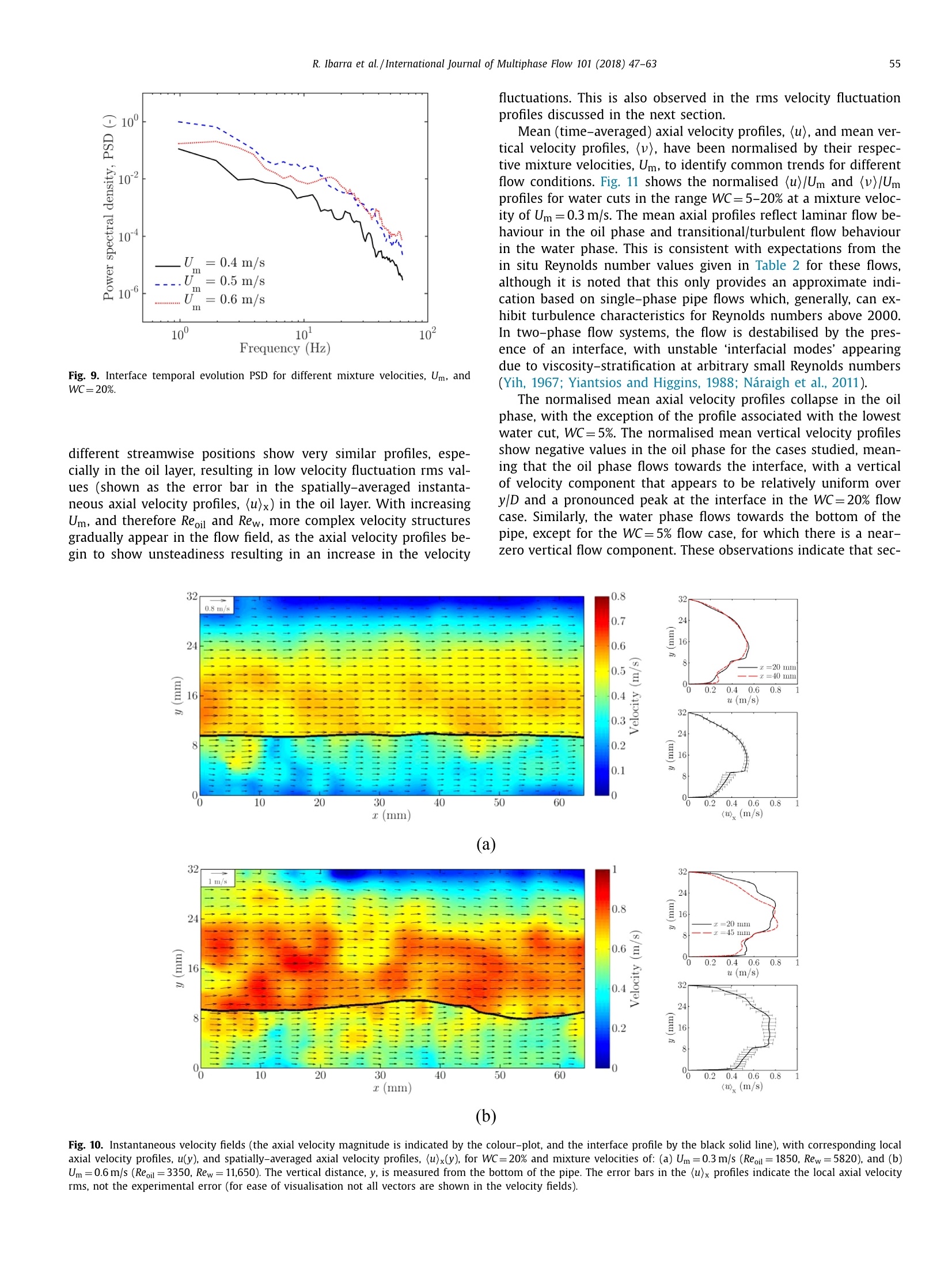
还剩15页未读,是否继续阅读?

产品配置单


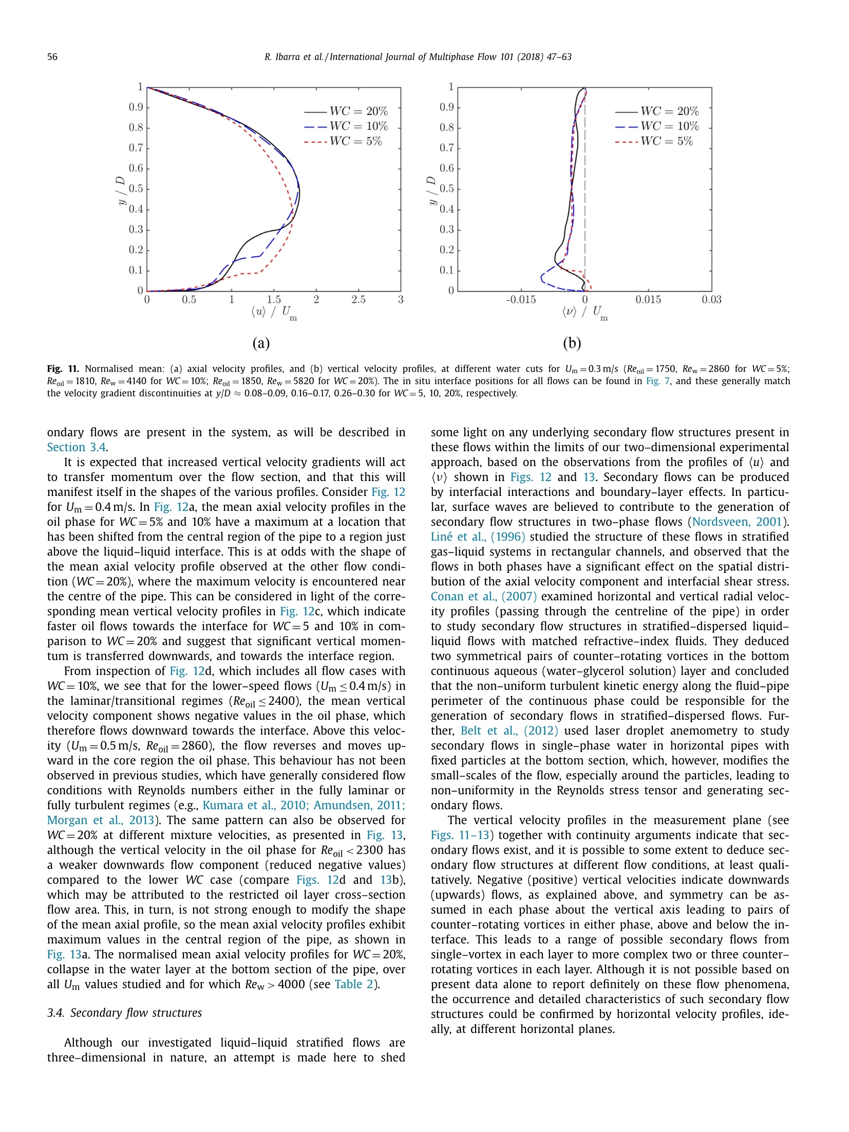
北京欧兰科技发展有限公司为您提供《水平管道中液 - 液流动中双线激光诱导荧光2-line PLIF,粒子成像测速PIV检测方案(气体流量计)》,该方案主要用于其他中双线激光诱导荧光2-line PLIF,粒子成像测速PIV检测,参考标准--,《水平管道中液 - 液流动中双线激光诱导荧光2-line PLIF,粒子成像测速PIV检测方案(气体流量计)》用到的仪器有PLIF平面激光诱导荧光火焰燃烧检测系统、德国LaVision PIV/PLIF粒子成像测速场仪、LaVision DaVis 智能成像软件平台
推荐专场


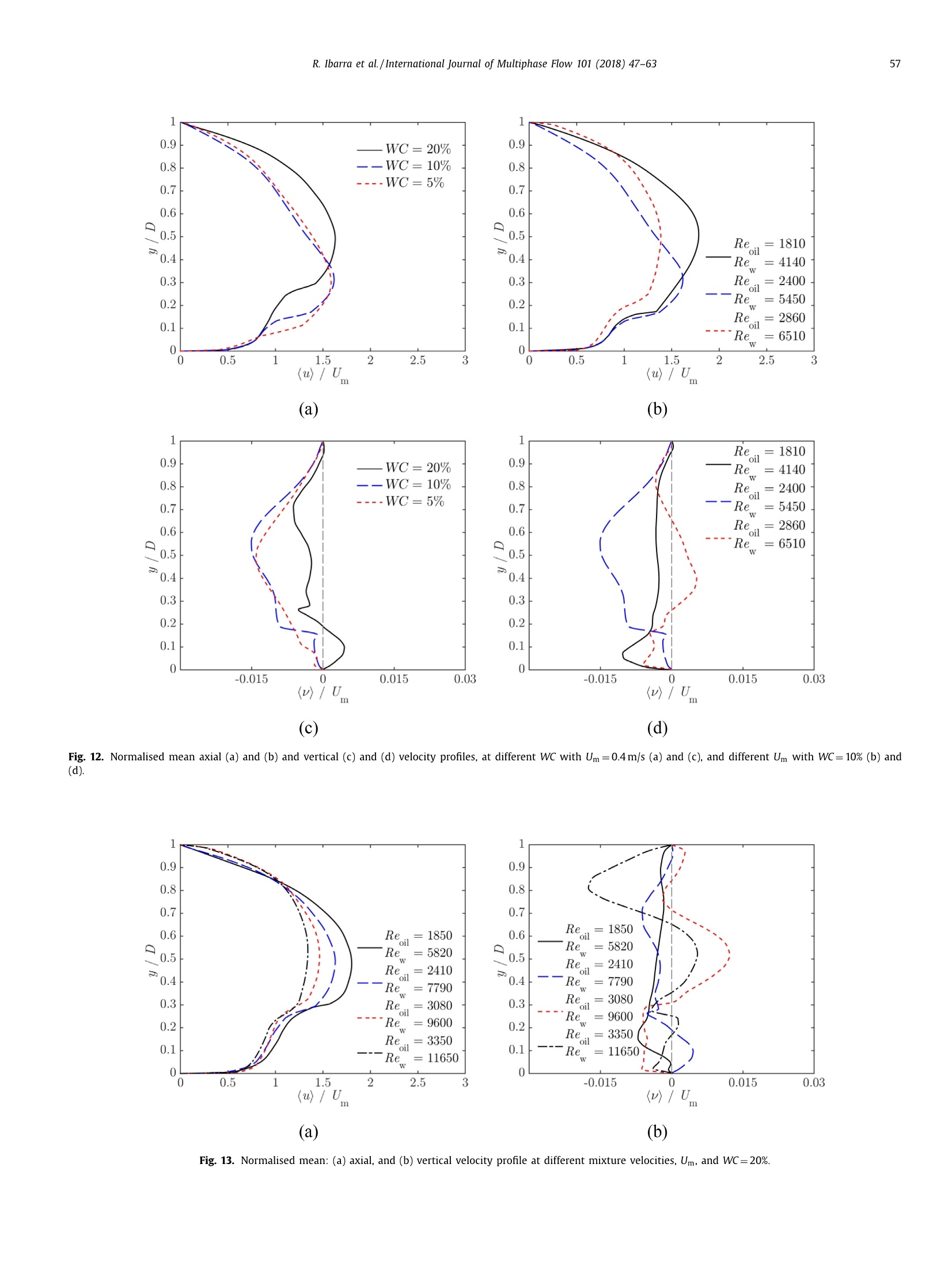
相关方案
更多
该厂商其他方案
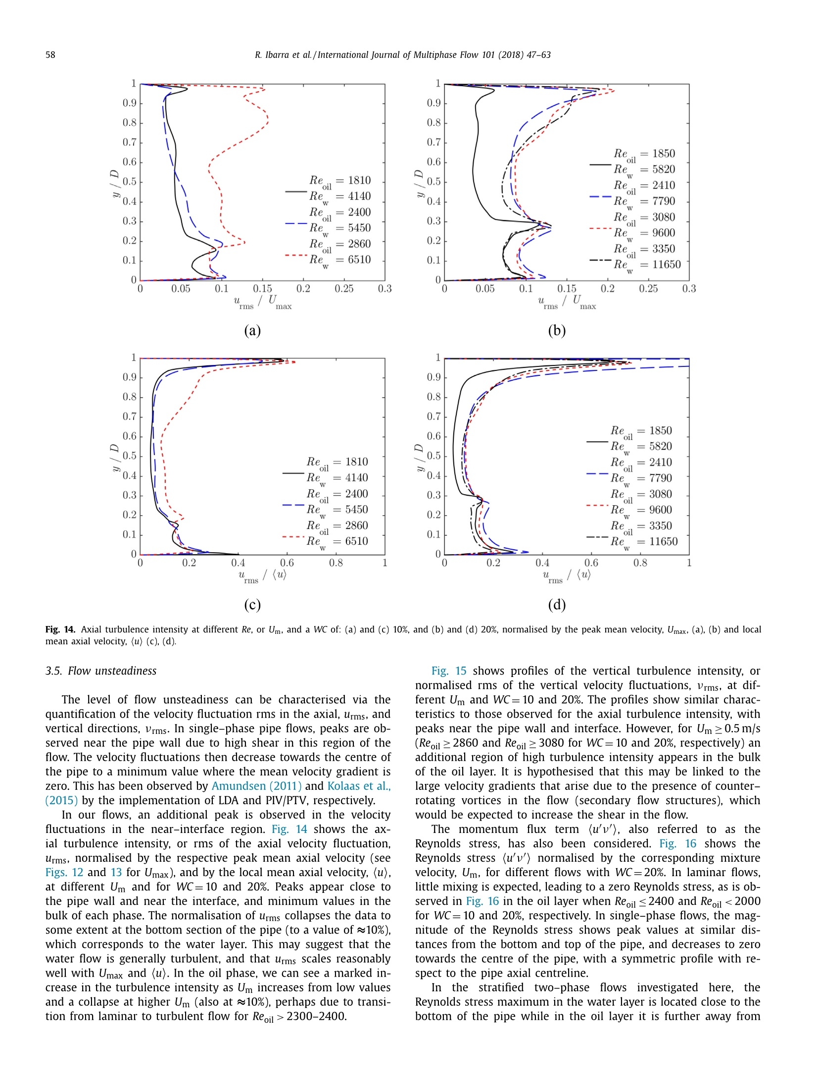
更多