


方案详情
文
采用4台高速相机和LaVision的DaVis8.2.0软件平台,构成一套时间分辨拉格朗日视角3D3C粒子跟踪测速系统。对拖曳水池中的翼型进行了实验测量,并进行了基于运动方程作为物理约束的拉格朗日数据梯度估算。
方案详情

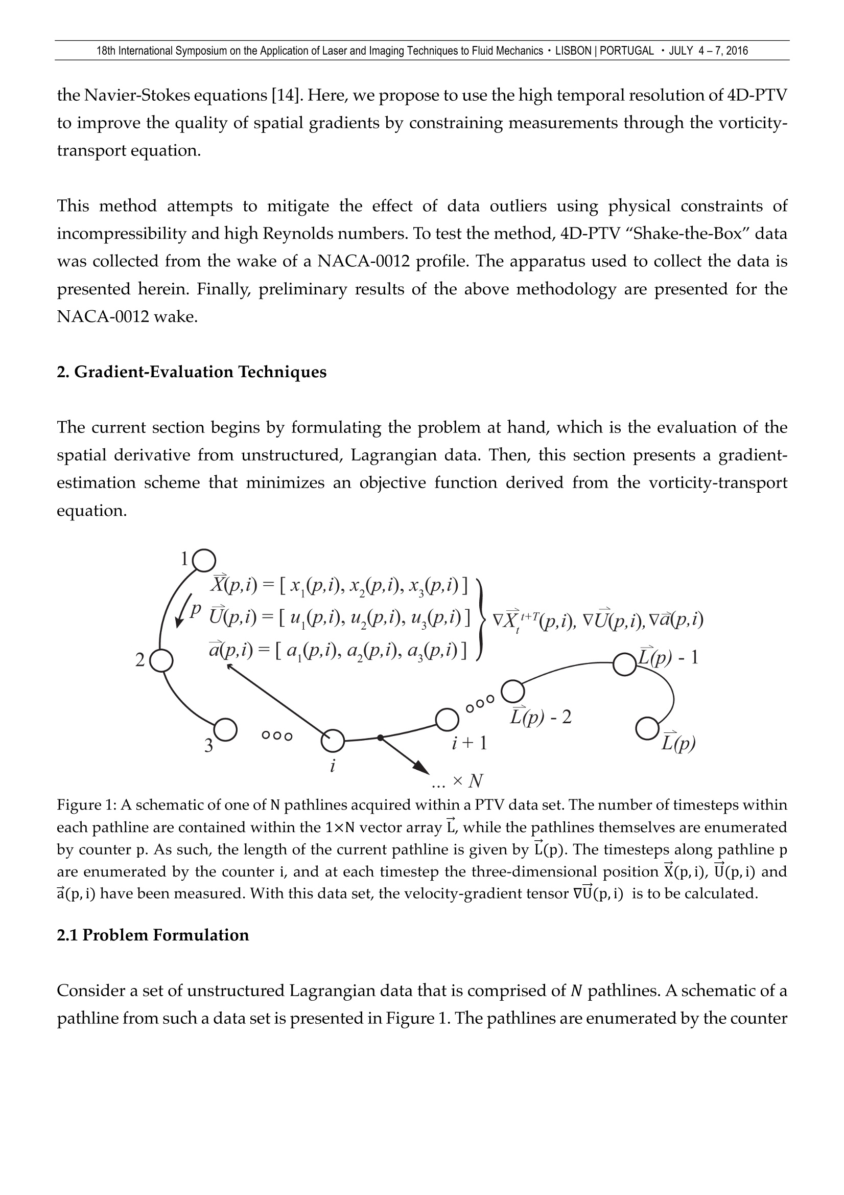
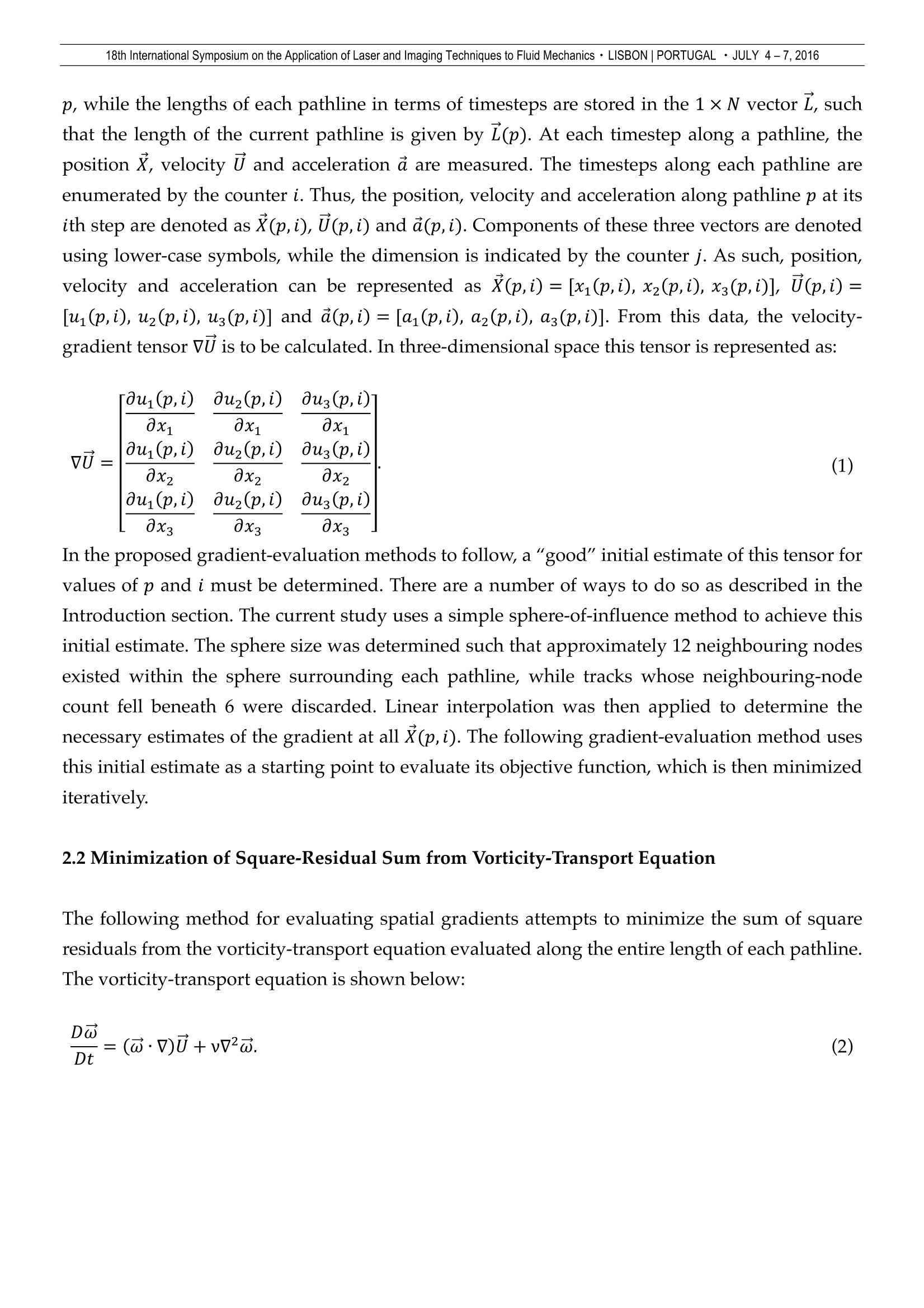
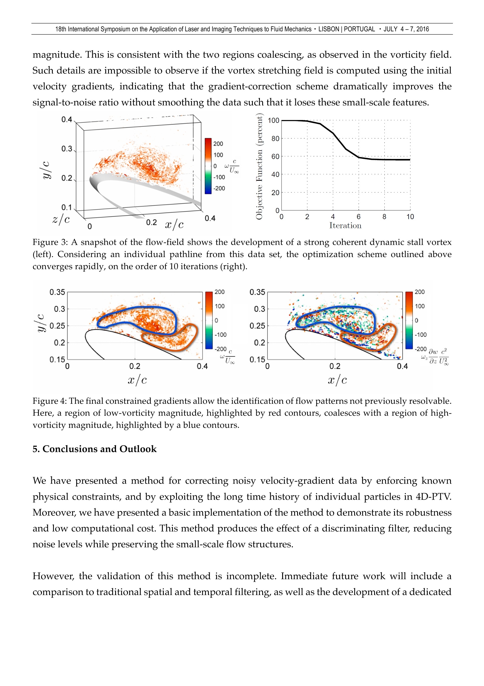
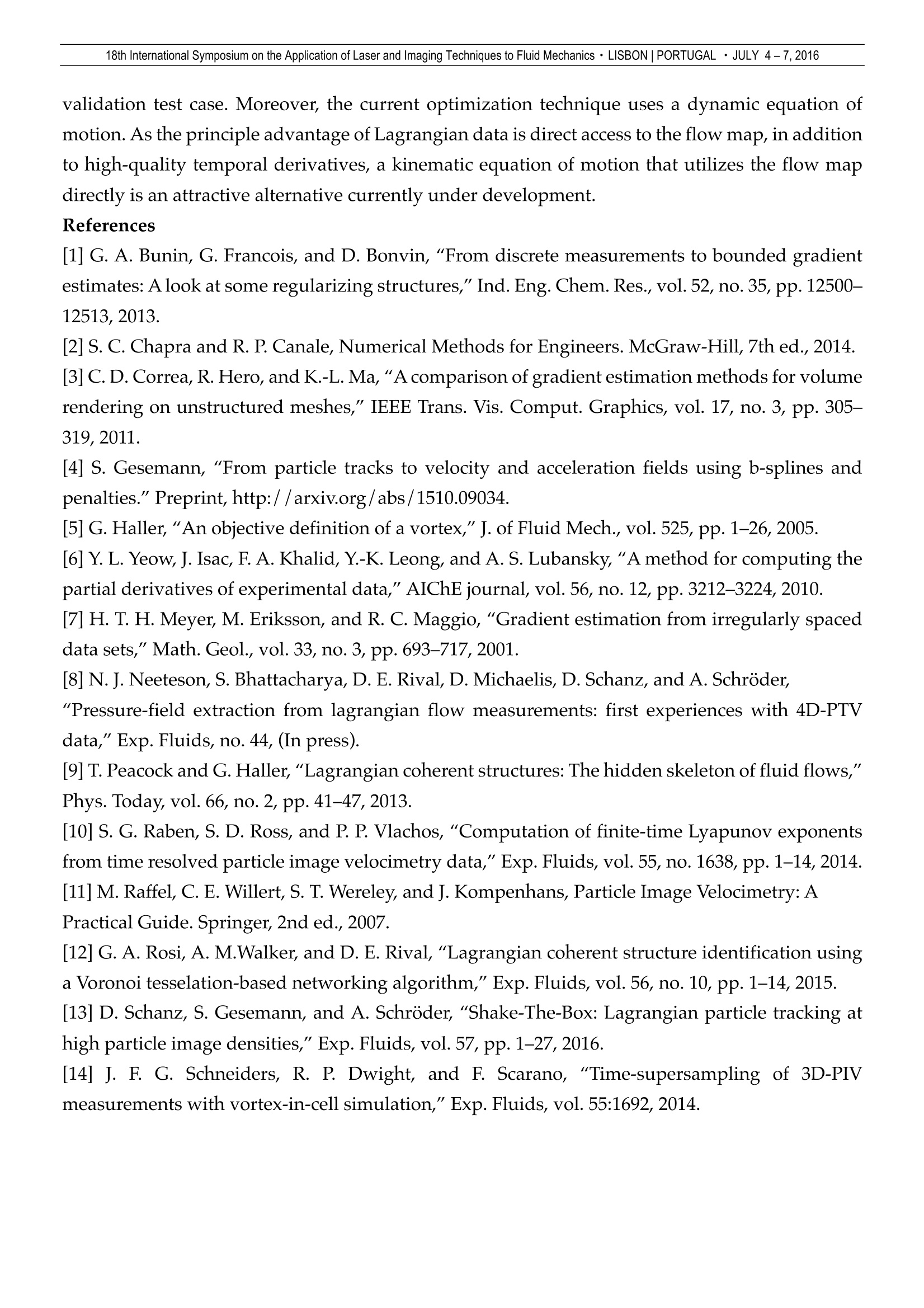
18th International Symposium on the Application of Laser and Imaging Techniques to Fluid Mechanics · LISBON|PORTUGAL ·JULY 4-7,2016 Gradient Estimation on Lagrangian Data Using Equations of Motion as PhysicalConstraints Jaime G. Wong, Giuseppe A. Rosi, David E. Rival Department of Mechanical and Materials Engineering, Queen’s University, Kingston, Canada *Correspondent author: jaime.wong@queensu.ca Keywords: Gradient estimation, flow-field reconstruction, physically constrained optimization ABSTRACT The advent of high-density particle tracking velocimetry has dramatically improved both spatial and temporalresolution available to researchers. However, making full use of the temporal data along a pathline does not yet exist.Here, a novel method for estimating gradients is proposed by applying equations of motion as constraints on theirvalues, while leveraging the substantial derivative along a pathline. Specifically, here we use the vorticity transportequation to limit the possible values of velocity-gradient components. It is shown that the method, althoughpreliminary, can reduce the noise in velocity gradients along a pathline and throughout a flow field. 1. Introduction Due to the ubiquity of particle image velocimetry (PIV), optical measurements have traditionallybeen used to acquire Eulerian flow-field data on a spatially uniform grid. In contrast, particletracking velocimetry (PTV) produces Lagrangian flow-field data on a spatially non-uniform grid.The advent of novel tracking algorithms such as "Shake-The-Box"has now made it possible toachieve spatial resolutions with 4D-PTV that are greater than Tomographic PIV [13]. With thespatial resolution of 4D-PTV now matching that of Tomo-PIV, it is reasonable to expect the wideradoption of PTV throughout the fluid-mechanics community. Collecting data in a Lagrangian frame presents with two significant advantages: it provides directaccess to the material derivative and to the flow map. Directly measuring the material derivativehas far-reaching applications. One such application is pressure extraction via the Poisson equation.In a Lagrangian frame, this operation can be performed accurately, since the material derivativeof velocity is directly measured. In contrast, if pressure is extracted from the material derivative inan Eulerian frame, one must be conscious of the possibility of compounding errors from themultiplication and summation of the many necessary measured terms [9]. Another application isin the study of entrainment across rotational non-rotational interfaces, since it is common practice to calculate the velocity of entrained fluid across the interface by normalizing the materialderivative of enstrophy by the magnitude of the enstrophy gradient [15]. Finally, having directaccess to the flow map is of particular use when calculating Lagrangian coherent structures [12],which are frame-invariant, user threshold-independent manifolds that separate a flow field intoregions of similar flow-map strain [9]. With Eulerian data, one is limited to Eulerian coherentstructures, which are both frame-variant and threshold-dependent [5]. One can attempt to acquirethe flow map from PIV data by synthetically seeding measured velocity fields with tracers andintegrating to determine their paths. However, this this method is limited due to the truncationerror and is computationally expensive [10]. However, PIV still offers one notable advantage over PTV, which is the ease and robustness ofspatial differentiation due to its spatially uniform grid. The uniform spacing of data nodes allowsone to quickly derive numerical representations of the spatial derivative, while the accuracy of thespatial derivative can be improved by using more data nodes surrounding a point of interest,which in turn reduces the residual error [2]. The uniform grid also simplifies spatial and temporalfiltering, which can in turn reduce the effect of data outliers on spatial differentiation. In contrast,the spatial non-uniformity of the data produced by PTV, which changes from time-step to time-step, makes spatial differentiation computationally slow and difficult to implement. Currently,typical methods to calculate the spatial derivative at a point of interest include: residual-minimization techniques that use an overdetermined system of equations based on neighboringnodes from which the spatial gradient can be calculated [6, 7]; or weighted-average techniquesthat calculate the gradient as a sum of weighted predictions based on neighboring nodes [3].Moreover, more sophisticated interpolation techniques make use of physical information aboutthe flow, such as a divergence-free velocity field, in order to improve resolution [4, 14]. The ability to mitigate the effect of data outliers remains an issue when calculating the spatialgradient on non-uniform data. Enforcing Lipschitz continuity on the gradient is likely the simplestmethod, while restraining the gradient to exist only within certain bounds is another [1]. However,applying these constraints aggressively can adversely affect the gradient, and thus information ofthe gradient should be known a priori, which may be unavailable. Furthermore, even if theseconstraints are placed conservatively, their lack of physical basis calls the accuracy of the resultinggradient into question. Thus, constraints that have some physical basis should be placed on theflow instead. For instance, it has been shown that tomographic PIV can be super-sampled belowthe Nyquist frequency by using the high spatial resolution to improve temporal resolution through the Navier-Stokes equations [14]. Here, we propose to use the high temporal resolution of 4D-PTVto improve the quality of spatial gradients by constraining measurements through the vorticity-transport equation. This method attempts to mitigate the effect of data outliers using physical constraints ofincompressibility and high Reynolds numbers. To test the method, 4D-PTV"Shake-the-Box" datawas collected from the wake of a NACA-0012 profile. The apparatus used to collect the data ispresented herein. Finally, preliminary results of the above methodology are presented for theNACA-0012 wake. 2. Gradient-Evaluation Techniques The current section begins by formulating the problem at hand, which is the evaluation of thespatial derivative from unstructured, Lagrangian data. Then, this section presents a gradient-estimation scheme that minimizes an objective function derived from the vorticity-transportequation. .×N Figure 1: A schematic of one of N pathlines acquired within a PTV data set. The number of timesteps withineach pathline are contained within the 1xN vector array L, while the pathlines themselves are enumeratedby counter p. As such, the length of the current pathline is given by L(p). The timesteps along pathline pare enumerated by the counter i, and at each timestep the three-dimensional position x(p,i), U(p,i) anda(p, i) have been measured. With this data set, the velocity-gradient tensor Vū(p,i) is to be calculated. 2.1 Problem Formulation Consider a set of unstructured Lagrangian data that is comprised of N pathlines. A schematic of apathline from such a data set is presented in Figure 1. The pathlines are enumerated by the counter p, while the lengths of each pathline in terms of timesteps are stored in the 1× N vector L, suchthat the length of the current pathline is given by L(p). At each timestep along a pathline, theposition X, velocity U and acceleration d are measured. The timesteps along each pathline areenumerated by the counter i. Thus, the position, velocity and acceleration along pathline p at itsith step are denoted as x(p,i),U(p,i) and a(p,i). Components of these three vectors are denotedusing lower-case symbols, while the dimension is indicated by the counter j. As such, position,velocity and acceleration can be represented as x(p,i)=[xi(p,i), x2(p,i), x3(p,i)], ū(p,i)=[ui(p,i), u2(p,i), u3(p,i)] and a(p,i)=[a1(p,i), az(p,i), a3(p,i)]. From this data, the velocity-gradient tensor VU is to be calculated. In three-dimensional space this tensor is represented as: In the proposed gradient-evaluation methods to follow, a"good" initial estimate of this tensor forvalues of p and i must be determined. There are a number of ways to do so as described in theIntroduction section. The current study uses a simple sphere-of-influence method to achieve thisinitial estimate. The sphere size was determined such that approximately 12 neighbouring nodesexisted within the sphere surrounding each pathline, while tracks whose neighbouring-nodecount fell beneath 6 were discarded. Linear interpolation was then applied to determine thenecessary estimates of the gradient at all X(p,i). The following gradient-evaluation method usesthis initial estimate as a starting point to evaluate its objective function, which is then minimizediterativelv. 2.2 Minimization of Square-Residual Sum from Vorticity-Transport Equation The following method for evaluating spatial gradients attempts to minimize the sum of squareresiduals from the vorticity-transport equation evaluated along the entire length of each pathline.The vorticity-transport equation is shown below: Da (2) At modest Reynolds numbers, the vorticity-diffusion term of this equation can be neglected. Thus,the substantial derivative and the vortex stretching term should be equal at all points along thepathline. However, due to the error in calculating the spatial derivative from the experimentaldata, these differences result in a residual for all dimensions j, and at every value of p and i. Theresiduals can be squared and summed, resulting in the single residual R (p, i) for a timestep alonga pathline: As R'(p, i) must be zero at all points along each pathline, these residuals can be summed along anentire pathline from 1 to p to produce an objective function 0 for the entire pathline. This functionis to be minimized. We wish to now find the set of VU(p, i) along the entire pathline the minimizes 0, given our initialguess. To do so, VO is first determined with respect to all nine elements of vū(p,i), along the entirelength of the pathline. Thus, VO is comprised of 9xL(p) equations. VO, which represents a singlecomponent equation of VO is presented in Eq. 5: 0 can thus be minimized by method of steepest descent by adjusting a step size alpha betweeniterations that minimizes 0 given the current gradient: The final estimates of VU(p,i) represent the evaluations of the velocity-gradient tensors along theentire pathline that have been corrected using information from other pathlines in its vicinity. While the method of steepest descent is very simple and only locally minimizing, it was chosenfor its ease of implementation, as it is sufficient to demonstrate the method proposed. Figure 2: A schematic of the water-filled towing tank and image-acquisition system used by the currentstudy to obtain 4D-PTV data. A NACA-0012 profile (A) was towed from rest through a measurementvolume located 15c downstream (B). The measurement volume was illuminated by 40mJ-per-pulse, 527nmlaser (C). The motions of 100um-diameter silver-coated glass microspheres were acquired by four FastcamSA-4 cameras at 1500Hz (D), from which 4D-PTV data of the wake was derived. 3. Apparatus: Towing-Tank Facility and Image-Acquisition System To test the gradient-evaluation methods presented in Sec. 2,"Shake-The-Box"4D-PTV data wascollected along the suction side of a towed NACA-0012 profile in a water-filled towing tank atQueen’s University. A schematic of the apparatus is shown in Figure 2. The span and chord of thewing wereL =1m andc= 0.3m, respectively, while the tip-gap spacing was kept less than 5%of chord, thereby ensuring a bulk two-dimensional flow. The profile was towed from rest with noinitial angle of attack at a constant velocity of 0.33m/s, corresponding to a chord-based Reynoldsnumber of Rec=105. The profile then pitched rapidlyytto an angle of attack ofα = 35° in order to form a strong dynamic stall vortex, such that physically sensible velocity-gradient estimates could be quickly identified from the large coherent structure. The profile’ssuction side passed through a 0.5cx0.5cx0.1c measurement volume arranged such that thenormal-vector of the laser plane was parallel with the span of the wing. The volume was located 15c downstream from the start position, thereby ensuring that the profile was in quasi-steadyconditions prior to the onset of motion. The measurement volume was achieved via a 40mJ-per-pulse, 527nm laser, which illuminated 100um-diameter silver-coated glass microspheres. Themotions of the microspheres were acquired by four Photron Fastcam SA-4 cameras sampling at1500Hz. The Stokes number of the particles was approximately 3×10⁻³《 0.1, which ensuredtracer-accuracy errors of <1% [11]. To minimize image distortions, water filled prisms were fixedonto the glass pane of the tank such that all cameras were orthogonal to a prism face. The imageswere then imported and processed in DaVis 8.2.0 (LaVision GmbH, Goettingen, Germany) for4DPTV analysis. Lagrangian data were subsequently exported to MATLAB 2012a (Mathworks,Natick, MA, USA) for post-processing. An initial estimate for the elements of the velocity-gradienttensor along the entire lengths of all pathlines was calculated using the sphere-of-influencemethod described in Sec. 2.1. As a proof-of-principle study, the gradient-evaluation method basedon the vorticity transport equation was applied to all pathlines. The proceeding section showspreliminary results achieved via this method. The second gradient-evaluation method that utilizesthe flow-map gradient is left as future work. 4. Results & Discussion An indicative flow-field snapshot prior to correction is shown in Figure 3, with the particle fieldcolored by spanwise vorticity. The dynamic stall vortex is shown clearly, and the particle tracks inthis region are long-lived, providing excellent temporal information for the physical constraintmethodology outlined above. A typical pathline optimization is also shown in Figure 3. As aconsequence of the gradient-descent method, only a local minimum of the objective function fromEquation (4) was obtained. However, this local minimum was obtained in under ten iterations,allowing the entire flow-field to be optimized within a few hours on a typical desktop PC. By enforcing the dynamic constraint of the vorticity equation, the spatial gradients observed in theflow field exhibit much greater coherence in both space and time. Specific flow patterns that couldnot be previously identified emerge, such as that exemplified by the flow field shown in Figure 4.Specifically, in the vorticity field, which is on the left of Figure 4, a region of low-vorticity fluidemerges. The region is highlighted by the red contour. This low-vorticity region coalesces with thehigh-vorticity dynamic stall vortex core, highlighted by the blue contour. The vortex core exhibitsvortex compression, corresponding to a reduction of vorticity magnitude. Meanwhile, the low-vorticity region is associated with vortex stretching, corresponding to an increase in vorticity magnitude. This is consistent with the two regions coalescing, as observed in the vorticity field.Such details are impossible to observe if the vortex stretching field is computed using the initialvelocity gradients, indicating that the gradient-correction scheme dramatically improves thesignal-to-noise ratio without smoothing the data such that it loses these small-scale features. -100 o-200.o Iteration Figure 3: A snapshot of the flow-field shows the development of a strong coherent dynamic stall vortex(left). Considering an individual pathline from this data set, the optimization scheme outlined aboveconverges rapidly, on the order of 10 iterations (right). Figure 4: The final constrained gradients allow the identification of flow patterns not previously resolvable.Here, a region of low-vorticity magnitude, highlighted by red contours, coalesces with a region of high-vorticity magnitude, highlighted by a blue contours. 5.Conclusions and Outlook We have presented a method for correcting noisy velocity-gradient data by enforcing knownphysical constraints, and by exploiting the long time history of individual particles in 4D-PTV.Moreover, we have presented a basic implementation of the method to demonstrate its robustnessand low computational cost. This method produces the effect of a discriminating filter, reducingnoise levels while preserving the small-scale flow structures. However, the validation of this method is incomplete. Immediate future work will include acomparison to traditional spatial and temporal filtering, as well as the development of a dedicated validation test case. Moreover, the current optimization technique uses a dynamic equation ofmotion. As the principle advantage of Lagrangian data is direct access to the flow map, in additionto high-quality temporal derivatives, a kinematic equation of motion that utilizes the flow mapdirectly is an attractive alternative currently under development. ( References ) ( [1] G. A. Bunin, G. Francois, an d D . Bonvin , “From discrete measurements to bounded gr a dientestimates: A look at some regularizing structures,"Ind. Eng. Chem. Res., vol. 5 2, no. 35,pp. 12500- 12513,2013. ) ( [2] S. C. Chapra and R. P. Canale, Numerical Methods for Engineers. McGraw-Hill, 7th ed., 2014. ) ( [3] C. D. Correa, R. Hero, and K.-L. Ma , "A comparison of gradient estimation methods for volumerendering on unstructured meshes," IEEE Trans. Vis. Comput. Graphics, vol. 17, n o . 3, pp. 305- 319,2011. ) ( [4] S. Gesemann, “From par t icle tracks to velocity and acceleration fields using b-sp l ines andpenalties."Preprint, http://arxiv.org/abs/1510.09034. ) ( [5] G. Haller,“An objective definition of a vortex,"J.of Fluid Mech., vol. 525, pp. 1-26, 2005. ) ( [6] Y.L. Yeow, J . Isac, F. A. Khalid, Y.-K. Leong, and A. S. Lubansky, “ A method for computing thepartial derivatives of experimental data," AIChE journal, vol. 56, no. 1 2 , pp. 3212-3224,2010. ) ( [7] H. T. H. Meyer, M. Eriksson, and R. C. Maggio,"Gradient estimation from irregularly spaceddata sets,"Math. Geol., vol. 33, no.3, pp. 693-717,2001. ) ( [8] N. J. Neeteson, S . Bhattacharya, D. E. Rival, D. Michaelis, D. Schanz, and A. Schroder,"Pressure-field extractio n from lagrangian flow measurements: first experiences with 4D-PTVdata," Exp. Fluids, no. 44, (In press). ) ( [9]T. Peacock and G. Haller, " Lagrangian coherent structures: The hidden skeleton of fluid flows,"Phys. Today, vol. 66, no. 2, pp. 41-47,2013. ) ( [10] S. G. Raben, S. D. Ross, and P. P. Vlachos,"Computation of finite-time Lyapunov exponentsfrom time resolved particle image velocimetry data,"Exp. Fluids, vol. 55, no. 163 8 ,pp. 1-14 , 2014.[11] M. Raffel, C. E. Willert, S. T. Wereley, and J. Kompenhans, Particle Image Velocimetry: APractical Guide. Springer, 2nd ed., 2007. ) ( [12] G. A. Rosi, A. M.Walker, and D. E. Rival,"Lagrangian coherent structure identification usinga Voronoi tesselation-based n e tworking algorithm"Exp.Fluids, vol. 56, no. 10, pp. 1-14, 2015. ) ( [13] D. Schanz, S. Gesemann, and A . Schroder, "Shake-The-Box: Lagrangian particle tracking athigh particle image densities," Exp. Fluids, vol. 57, pp. 1-27, 2016. ) ( [14] J. F. G. Schneiders, R. P. Dwight, and F. S carano, “Time-supersampling of 3D - PIVmeasurements with vortex-in-cell simulation," Exp. Fluids, vol. 55:1692, 2014. ) [15] M. Wolf, M. Holzner, D. Krug, B. Liithi, W. Kinzelbach, and A. Tsinober, "Effects of mean shearon the local turbulent entrainment process,"J. Fluid Mech., vol. 731, pp. 95-116, July 2013. The advent of high-density particle tracking velocimetry has dramatically improved both spatial and temporal resolution available to researchers. However, making full use of the temporal data along a pathline does not yet exist. Here, a novel method for estimating gradients is proposed by applying equations of motion as constraints on their values, while leveraging the substantial derivative along a pathline. Specifically, here we use the vorticity transport equation to limit the possible values of velocity-gradient components. It is shown that the method, although preliminary, can reduce the noise in velocity gradients along a pathline and throughout a flow field.
确定
还剩8页未读,是否继续阅读?

产品配置单


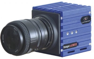
北京欧兰科技发展有限公司为您提供《拖曳水池中3D3C速度矢量场检测方案(CCD相机)》,该方案主要用于其他中3D3C速度矢量场检测,参考标准--,《拖曳水池中3D3C速度矢量场检测方案(CCD相机)》用到的仪器有Imager sCMOS PIV相机、体视层析粒子成像测速系统(Tomo-PIV)、LaVision DaVis 智能成像软件平台
推荐专场
CCD相机/影像CCD
更多


相关方案
更多
该厂商其他方案
更多