分形格栅生成湍流中速度矢量场检测方案(CCD相机)

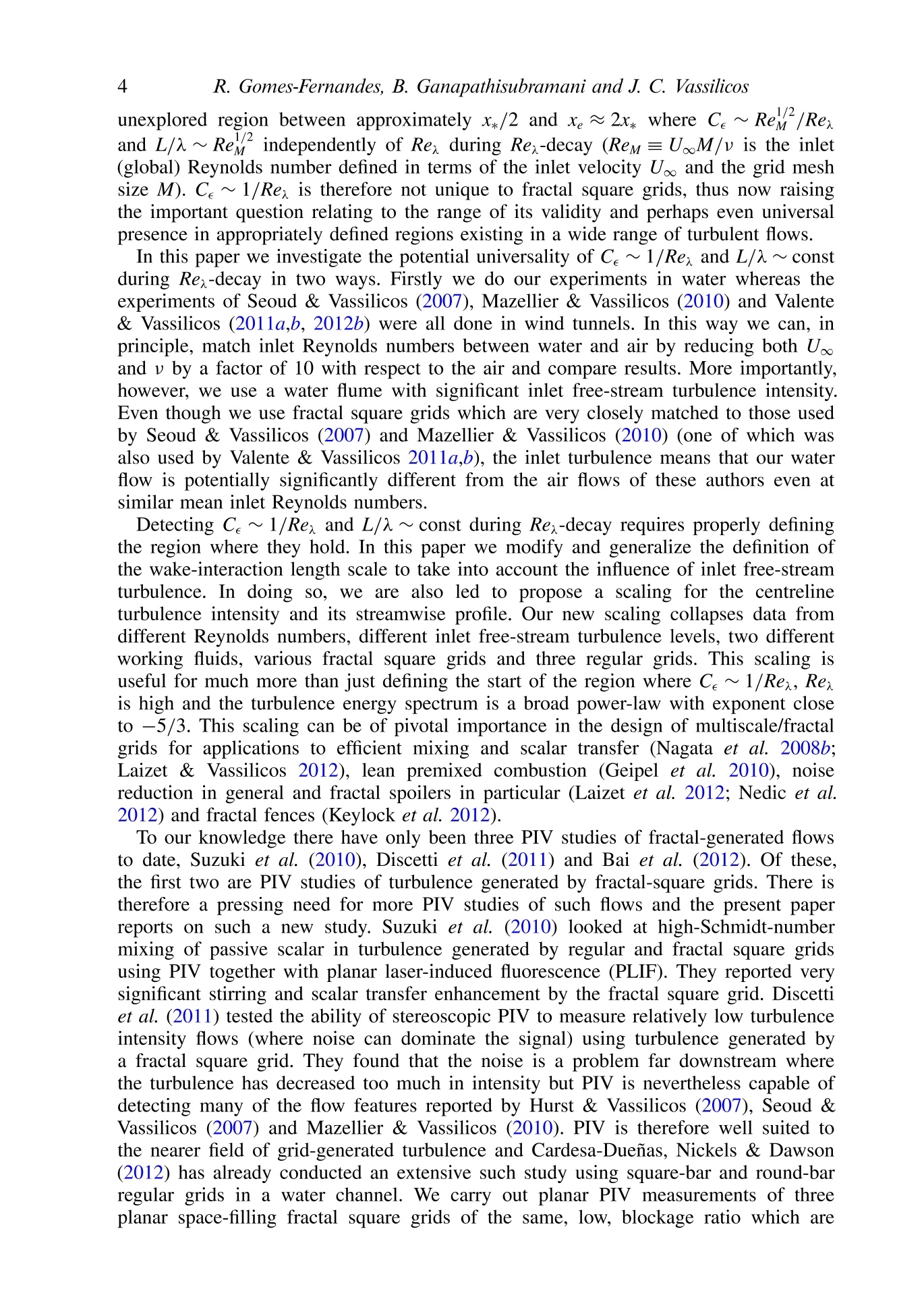
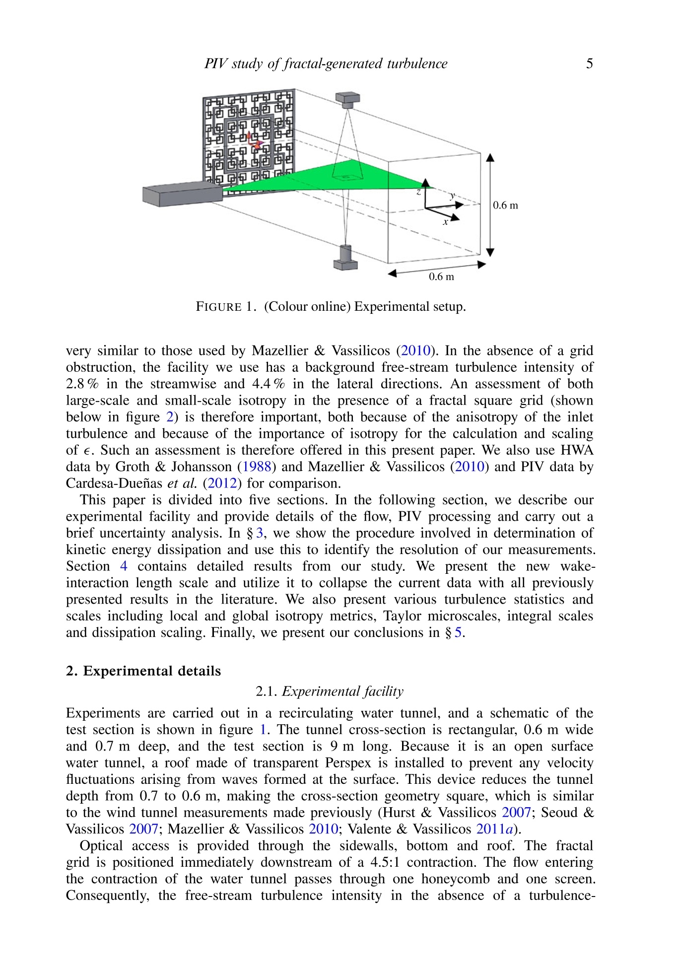
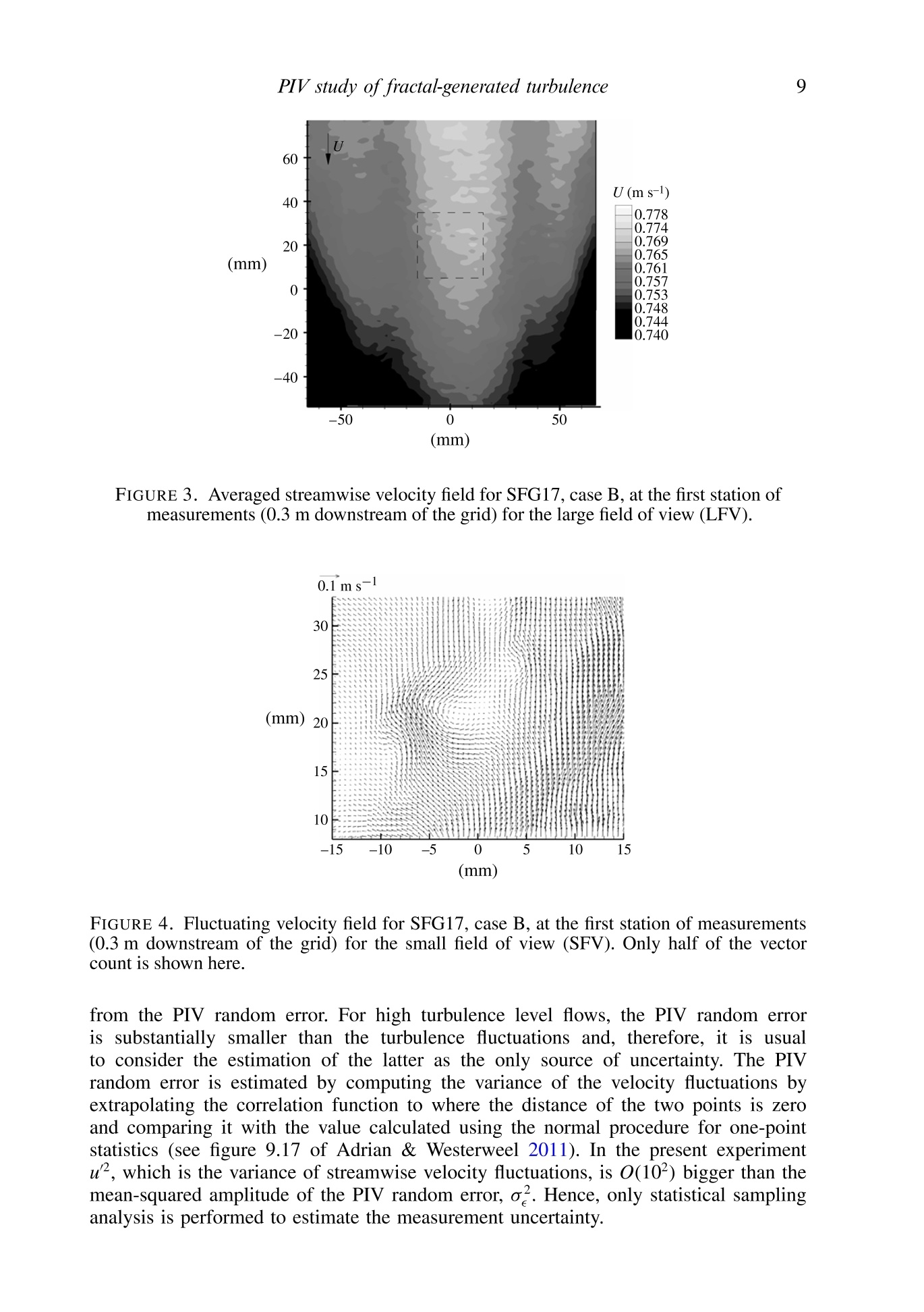
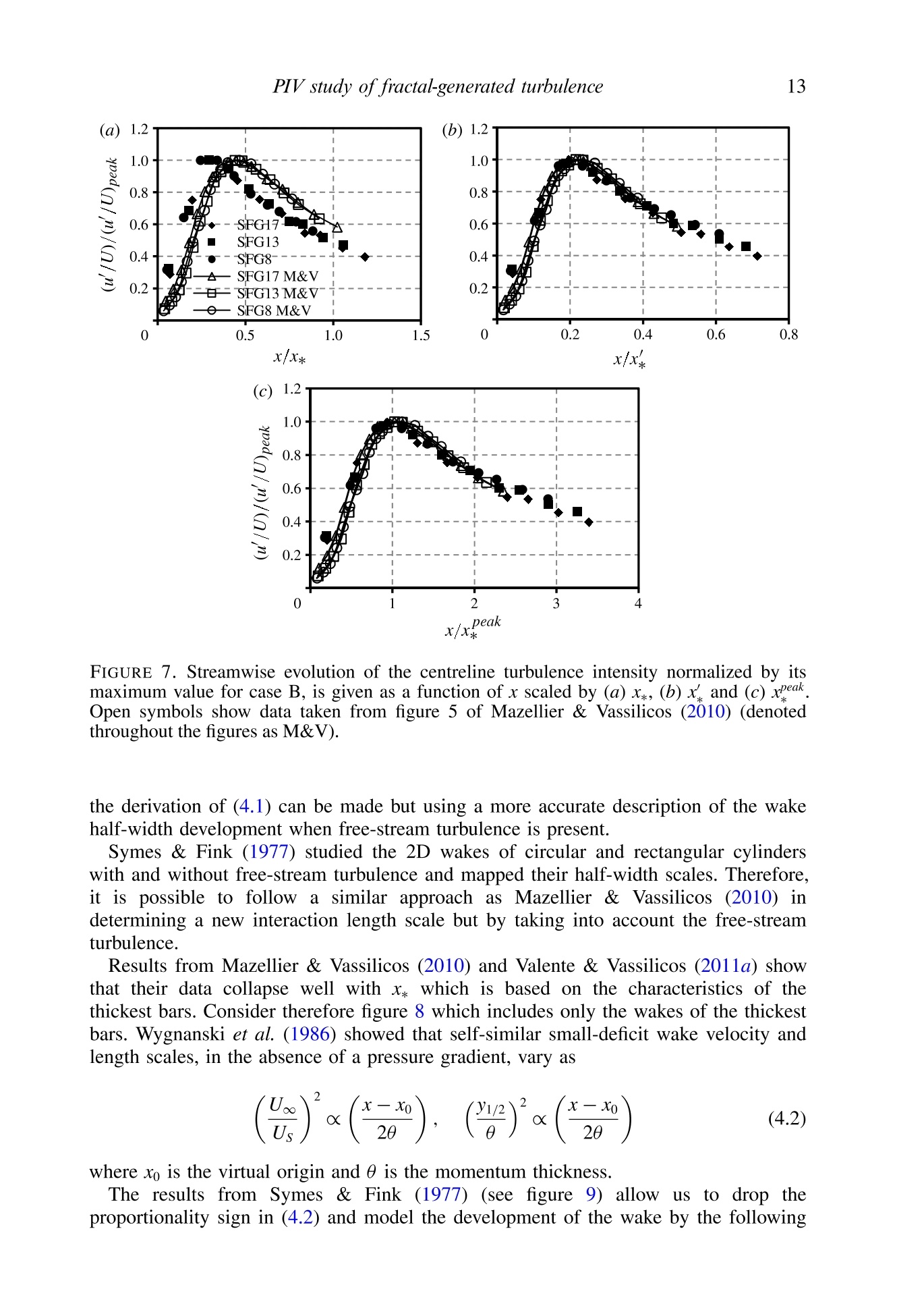
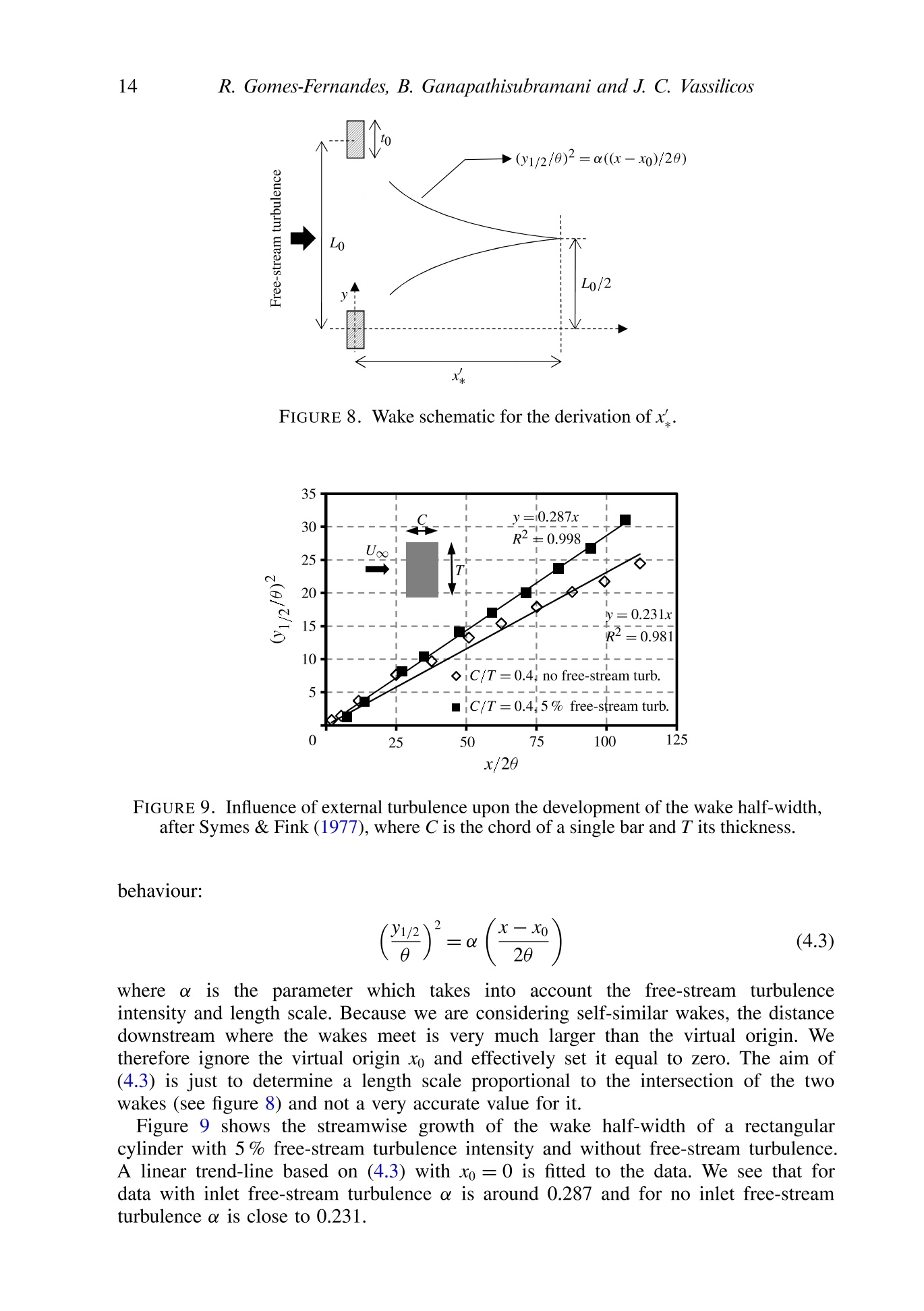
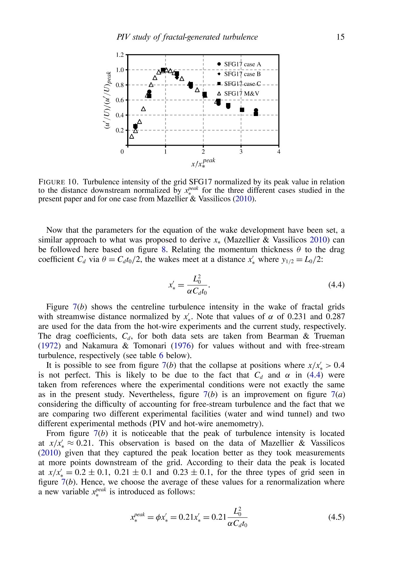
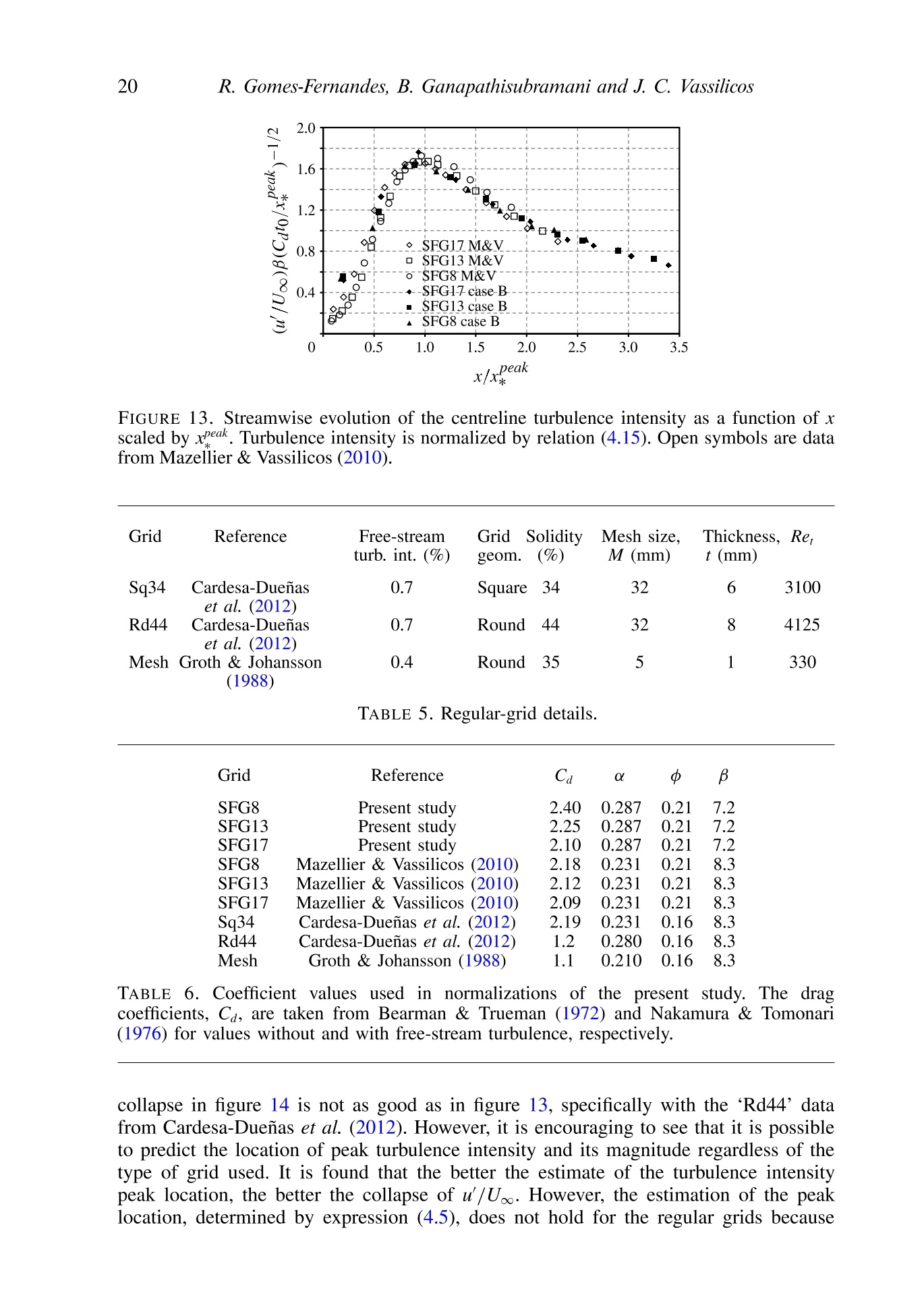
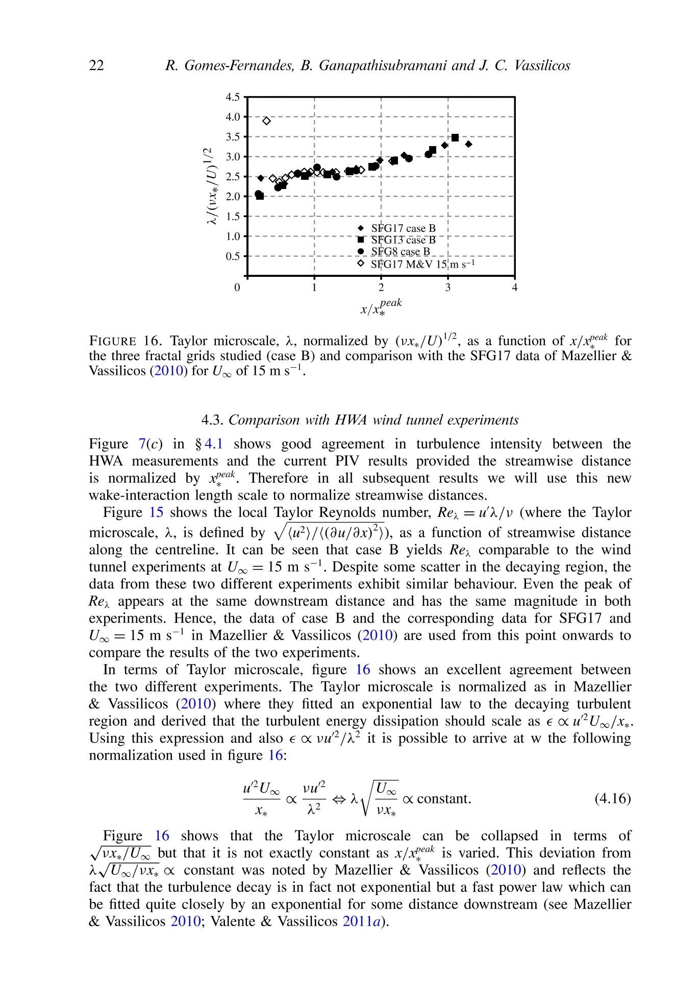
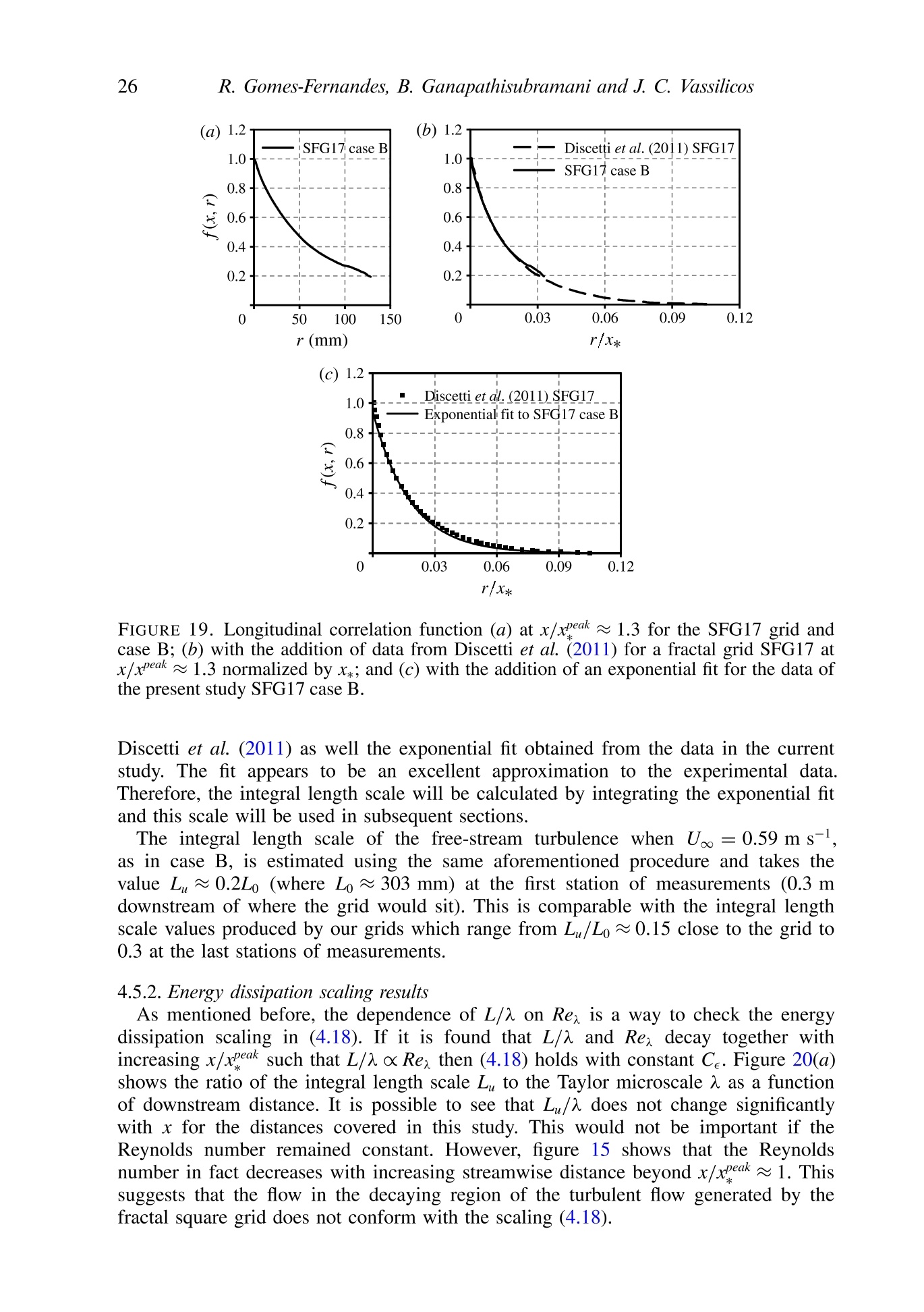
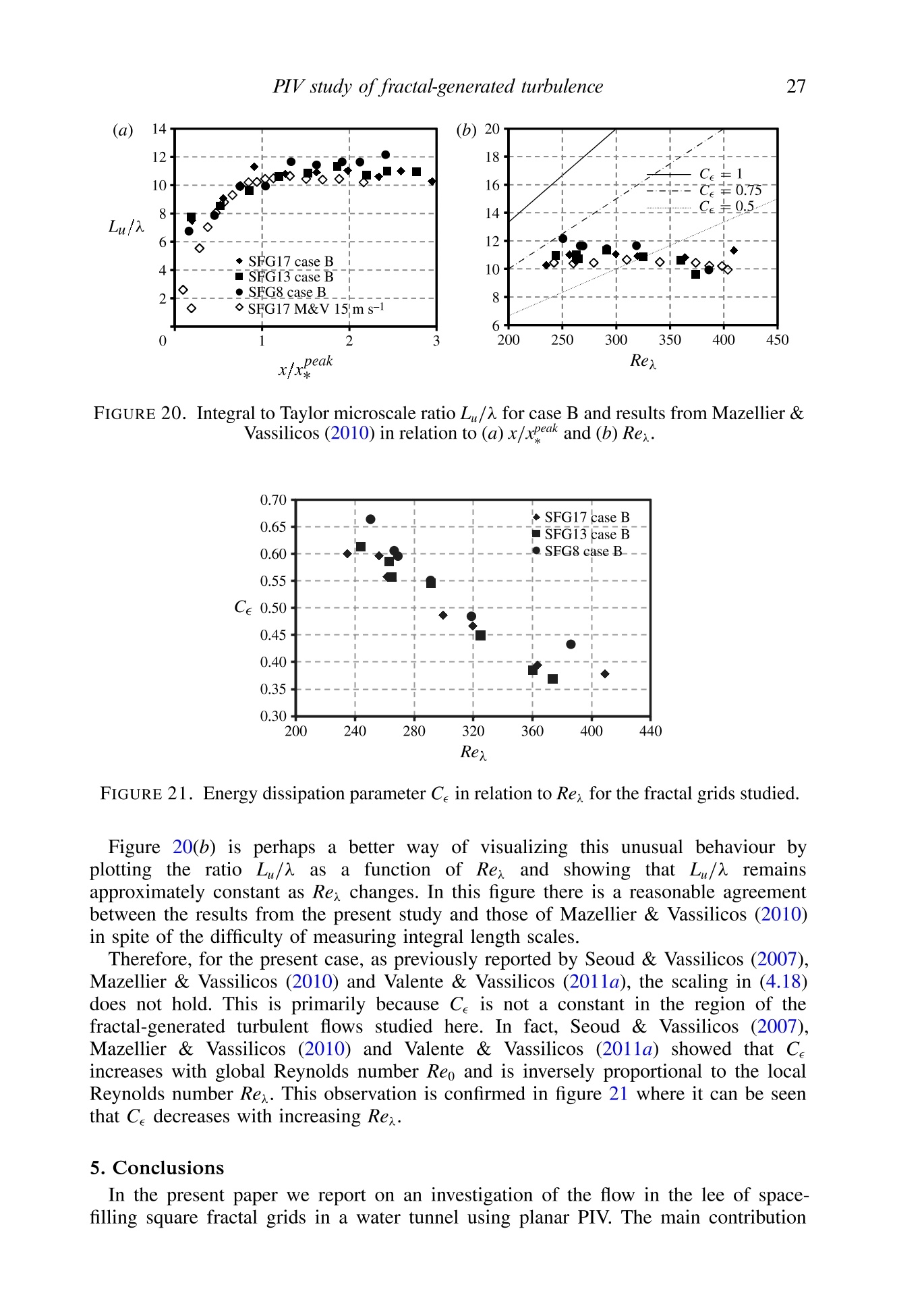
J. Fluid Mech.， page 1 of 31.C Cambridge University Press 2012doi：10.1017/jfm.2012.394 2R. Gomes-Fernandes， B. Ganapathisubramani and J. C. Vassilicos Journal of Fluid Mechanics http：//journals.cambridge.org/FLM Additional services for Journal of Fluid Mechanics： Email alerts： Click here Subscriptions： Click here Commercial reprints： Click here Terms of use ： Click here Particle image velocimetry study of fractal-generatedturbulence R. Gomes-Fernandes， B. Ganapathisubramani and J. C. Vassilicos Journal of Fluid Mechanics /FirstView Article / September 2012， pp 1-31DOI： 10.1017/jfm.2012.394， Published online： Link to this article： http：//journals.cambridge.org/abstract S0022112012003941 How to cite this article： R. Gomes-Fernandes， B. Ganapathisubramani and J. C. Vassilicos Particle image velocimetrystudy of fractal-generated turbulence. Journal of Fluid Mechanics， Available on CJO doi：10.1017/ifm.2012.394 CAMBRIDGE Particle image velocimetry study offractal-generated turbulence R. Gomes-Fernandes t， B. Ganapathisubramaniand J. C. Vassilicos Department of Aeronautics， Imperial College London， London SW7 2AZ， UK Aerodynamics & Flight Mechanics Research Group， University of Southampton，Southampton SO17 1BJ， UK (Received 18 April 2012； revised 31 July 2012； accepted 1 August 2012) An experimental investigation involving space-filling fractal square grids is presented.The flow is documented using particle image velocimetry (PIV) in a water tunnel asopposed to previous experiments which mostly used hot-wire anemometry in windtunnels. The experimental facility has non-negligible incoming free-stream turbulence(with 2.8 %and 4.4% in the streamwise (u'/U) and spanwise (v’/U) directions，respectively) vwhich presents a challenge in terms of comparison withpreviouswind tunnel results. An attempt to characterize the effects of the incoming freestream turbulence on the grid-generated turbulent flow is made and an improvedwake-interaction length scale isproposed which eennaabblleess tthe comparison of thepresent results with previous ones for both fractal square and regular grids. Thislength scale also proves to be a good estimator of the turbulence intensity peaklocation. Furthermore， a new turbulence intensity normalization capable of collapsingu/U for various grids in various facilities is proposed. Comparison with previousexperiments indicates good agreement in turbulence intensities， Taylor microscale， aswell as various other quantities， if the improved wake-interaction length scale is used.Global and local isotropy of fractal-generated turbulence is assessed using the velocitygradients of the two-component (2C) two-dimensional (2D) PIV and compared withregular grid results. Finally， the PIV data appear to confirm the new dissipationbehaviour previously observed in hot-wire measurements. Key words： turbulence control， turbulence theory， wakes 1. Introduction The study of turbulent flows originating from a fractal object obstructing a steadylaminar stream started with Queiros-Conde & Vassilicos (2001) and Staicu et al.(2003) who took turbulence measurements in the wake of three-dimensional fractalbranching tree-like objects. This was followed by some early fractal/multiscale-forcedturbulence simulations by Mazzi， Okkels & Vassilicos (2002)， Biferale et al. (2004)and Mazzi & Vassilicos (2004) and， after a few years， led to the first ever studyof turbulence generated by planar fractal/multiscale grids (Hurst & Vassilicos 2007).Hurst & Vassilicos (2007) experimented with three different families of planar fractalgrids： fractal cross-grids， fractal I-grids and fractal square grids (see figure 2 for thelatter). They tried a total of 21 grids and reported unusual/unconventional properties only for their fractal square grids. As a result， the majority of subsequent studiesof fractal-grid-generated turbulence have concentrated on fractal square grids (Seoud& Vassilicos 2007； Nagata et al. 2008a，b； Laizet， Lamballais & Vassilicoss 2010Mazellier & Vassilicos 2010； Stresing et al. 2010； Suzuki et al. 2010； Discetti et al.2011； Laizet & Vassilicos2011；Valente & Vassilicos22011a，b； Laizet et al. 2012；Laizet & Vassilicos ：2012). Even so， there have been a couple of studies whichused multiscale/fractal cross-grids to enhance the Reynolds number (Geipel， Goh &Lindstedt 2010； Kinzel et al. 2011) and one set of high-quality measurements veryfar downstream of regular and multiscale cross-grids which has provided the mostcompelling data to date demonstrating the far downstream dependence of turbulencedecay on inlet conditions (see Valente & Vassilicos2012a) as originally proposedby George (1992). The measurements of pressure drop across planar fractalgridsof Hurst & Vassilicos (2007) also motivated Aly， Chong， Nicolleau & Beck (2010)，Nicolleau， Salim & Nowakowski (2011) and Zheng， Nicolleau & Qin (2012) tostudy the pressure drop across fractal-shaped orifices in turbulent pipe flows. Kang，Dennis & Meneveau (2011) measured drag forces on fractal Sierpinski carpets andtriangles which look very similar to some of the fractal-shaped orifices used by Alyet al. (2010) and Nicolleau et al. (2011). Anderson & Meneveau (2011) studied andmodelled flows over fractal-like multiscale surfaces. The planar fractal I-grids introduced by Hurst & Vassilicos (2007)：are two-dimensional analogues of the three-dimensional fractal branching tree-like structuresused by Queiros-Conde & Vassilicos (2001). Whereas there has been no study ofturbulence generated by fractal I grids since Hurst & Vassilicos (2007) (except forMazellier & Vassilicos 2008 who used fractal I grid and fractal cross-grid data byHurst & Vassilicos 2007 in their demonstration of the inlet-condition dependence ofthe turbulence dissipation constant)， there has been some work starting with Chester，Meneveau & Parlange (2007) and Chester & Meneveau (2007) on fractal trees whichare not dissimilar to the fractal I trees of Queiros-Conde & Vassilicos (2001). Thefocus of that work has been on the calculation of drag forces using renormalizednumerical simulation to model the drag of unresolved branches of the fractal tree.More recently， particle image velocimetry (PIV) measurements were carried out in thenear wake of a fractal-like tree demonstrating the importance of the tree’s multiscalestructure for the actual modelling of the flow (Bai， Meneveau & Katz 2012). One of the motivations of the original experiments by Queiros-Conde & Vassilicos(2001) aand of the early simulations by Mazzi & Vassilicos (2004)， but alsoof much of the hot-wire anemometry (HWA)work which followed using fractalsquare grids (Seoud & Vassilicos2007；Mazellier & Vassilicos32010；VVaalente &Vassilicos2011a，b)， was to generate hitherto unexplored turbulent flow conditionswhere the high-Reynolds-number scaling of the kinetic energy dissipation e mightbe significantly different from the conventionale~ K3/2/L (where K and L are，respectively， the turbulent kinetic energy and some local correlation length scale).This scaling is referred to as one of the cornerstone assumptions of turbulence theory'by Tennekes & Lumley (1972)， and Batchelor (1953) comments that it suggests thatenergy transfer occurs chiefly as a result of inertial interactions of wavenumbersof the same order of magnitude’. Interestingly， Doering & Foias (2002) rigorouslyproved from the incompressible Navier-Stokes equations that periodic and statisticallystationary body-forced three-dimensional turbulence is such that eX*/2 which has yet to be determined. Mazellier & Vassilicos(2010) also showed that the constant value taken by L/ during Re -decay is in fact anincreasing function of the inlet velocity， U.. Valente & Vassilicos (2012b) applied the wake-interaction length scale to theanalysis of turbulencgeenerated by regular gridsand found a hitherto largely unexplored region between approximately x*/2 and xe~ 2x where Ce~ReM /Reand L/入~ ReM independently of Re during Rex-decay (ReM =UM/v is the inlet(global) Reynolds number defined in terms of the inlet velocity U. and the grid meshsize M). C~1/Re is therefore not unique to fractal square grids， thus now raisingthe important question relating to the range of its validity and perhaps even universalpresence in appropriately defined regions existing in a wide range of turbulent flows. In this paper we investigate the potential universality of Ce~1/Re， and L/~ constduring Re-decay in two ways. Firstly we do our experiments in water whereas theexperiments of Seoud & Vassilicos (2007)， Mazellier & Vassilicos (2010) and Valente& Vassilicos (2011a，b， 2012b) were all done in wind tunnels. In this way we can， inprinciple， match inlet Reynolds numbers between water and air by reducing both U.and p by a factor of 10 with respect to the air and compare results. More importantly，however， we use a water flume with significant inlet free-stream turbulence intensityEven though we use fractal square grids which are very closely matched to those usedby Seoud & Vassilicos (2007) and Mazellier & Vassilicos (2010) (one of which wasalso used by Valente & Vassilicos 2011a，b)， the inlet turbulence means that our waterflow is potentially significantly different from the air flows of these authors even atsimilar mean inlet Reynolds numbers. Detecting Ce~1/Rex and L/A~ const during Re-decay requires properly definingthe region where they hold. In this paper we modify and generalize the definitionA ofthe wake-interaction length scale to take into account the influence of inlet free-streamturbulence. In doing so， we are also led to propose a scaling for the centrelineturbulence intensity and its streamwise profile. Our new scaling collapses data fromdifferent Reynolds numbers， different inlet free-stream turbulence levels， two differentworking fluids， various fractal square grids and three regular grids. This scaling isuseful for much more than just defining the start of the region where Ce~1/Re， Rexis high and the turbulence energy spectrum is a broad power-law with exponent closeto -5/3. This scaling can be of pivotal importance in the design of multiscale/fractalgrids for applications to efficient mixing and scalar transfer (Nagata et al. 2008b；izet & Vassilicos 2012)， lean premixed combustion (Geipel et al. 2010)， O1reduction in general and fractal spoilers in particular (Laizet et al. 2012； Nedic et al.2012) and fractal fences (Keylock et al. 2012). To our knowledge there have only been three PIV studies of fractal-generated flowsto date， Suzuki et al. (2010)， Discetti et al. (2011) and Bai et al. (2012). Of these，the first two are PIV studies of turbulence generated by fractal-square grids. There istherefore a pressing need for more PIV studies of such flows and the present paperreports on such a new study. Suzuki et al. (2010) looked at high-Schmidt-numbermixing of passive scalar in turbulence generated by regular and fractal square gridsusing PIV together with planar laser-induced fluorescence (PLIF). They reported verysignificant stirring and scalar transfer enhancement by the fractal square grid. Discettiet al. (2011) tested the ability of stereoscopic PIV to measure relatively low turbulenceintensity flows (where noise can dominate the signal) using turbulence generated bya fractal square grid. They found that the noise is a problem far downstream wherethe turbulence has decreased too much in intensity but PIV is nevertheless capable ofdetecting many of the flow features reported by Hurst & Vassilicos (2007)， Seoud &Vassilicos (2007) and Mazellier & Vassilicos (2010). PIV is therefore well suited tothe nearer field of grid-generated turbulence and Cardesa-Duenas， Nickels & Dawson(2012) has already conducted an extensive such study using square-bar and round-barregular grids in a water channel. We carry out planar PIV measurements of three.planar space-filling fractal square grids of the same， low， blockage ratio which are FIGURE 1. (Colour online) Experimental setup. very similar to those used by Mazellier & Vassilicos (2010). In the absence of a gridobstruction， the facility we use has a background free-stream turbulence intensity of2.8% in the streamwise and 4.4% in the lateral directions. An assessment of bothlarge-scale and small-scale isotropy in the presence of a fractal square grid (shownbelow in figure 2) is therefore important， both because of the anisotropy of the inletturbulence and because of the importance of isotropy for the calculation and scalingof e. Such an assessment is therefore offered in this present paper. We also use HWAdata by Groth & Johansson (1988) and Mazellier & Vassilicos (2010) and PIV data byCardesa-Duenas et al.(2012) for comparison. This paper is divided into five sections. In the following section， we describe ourexperimental facility and provide details of the flow， PIV processing and carry out abrief uncertainty analysis. In 83， we show the procedure involved in determination ofkinetic energy dissipation and use this to identify the resolution of our measurements.Section 4contains detailed results from our study. We wake-interaction length scale and utilize it to collapse the current data with all previouslypresented results in the literature. We also present various turbulence statistics andscales including local and global isotropy metrics， Taylor microscales， integral scalesand dissipation scaling. Finally， we present our conclusions in $ 5. 2. Experimental details 2.1. Experimental facility Experiments are carried out in a recirculating water tunnel， and a schematic of thetest section is shown in figure1. The tunnel cross-section is rectangular， 0.6 m wideand 0.7 m deep， and the test section is 9 m long. Because it is an open surfacewater tunnel， a roof made of transparent Perspex is installed to prevent any velocityfluctuations arising from waves formed at the surface. This device reduces the tunneldepth from 0.7 to 0.6 m， making the cross-section geometry square， which is similarto the wind tunnel measurements made previously (Hurst & Vassilicos2007； Seoud &Vassilicos2007； Mazellier & Vassilicos 2010； Valente & Vassilicos 2011a). Opticalaccess is provided through the sidewalls， bottom and roof. The fractalgrid is positioned immediately downstream of a 4.5：1 contraction. The flow enteringthe contraction of the water tunnel passes through one honeycomb and one screen.Consequently， the free-stream turbulence intensity in the absence of a turbulence- TABLE 1. Free-stream velocities and Re for the three experimental cases. SFG8， SFG13and SFG17 are the three grids tested. Reo and ReL are the Reynolds numbers based on thethickness to and on the distance Lo between the thickest bars， respectively (see figure 2 forgeometrical details)， i.e.Reo=U.oto/v and Re =U.Lo/v. generating grid is up to 2.8% for the streamwise fluctuating velocity u and 4.4% forthe spanwise fluctuating velocity v. These estimates were obtained by carrying out PIVmeasurements immediately downstream of the contraction without the fractal grid. Theturbulence intensity in the streamwise direction (u/U) peaks 1.8 m downstream of thegrid with a value of 3.2 % whereas the turbulence intensity in the spanwise direction(u'/U) always decreases and has a value of 3.7% at the same distance downstream，1.8 m. The presence of non-negligible free-stream turbulence presents an opportunity. Onthe one hand， it might affect results in a way that might not allow comparisonwith previous wind tunnel low inlet free-stream turbulence experiments. On the otherhand， if the fractal grids， in some sense，‘‘break’the incoming turbulence and if theturbulence behaves thereafter as in previous experiments， that would be a significantresult. It must be noted that most of the analysis carried out in this study requires access tothe inlet speed(U). This speed is used to normalize various quantities in subsequentsections. However， we are unable to measure the inlet speed upstream of the griddue to lack of opticalaccess.. ITherefore， it is not possible to compare data fromthe wind tunnel experiments with the present one based only， for example， on aglobal Reynolds number Reo=f(U，l，v) (where is an appropriate length scalecharacteristic of the grid and vis the kinematic viscosity of the fluid). On the otherhand， we do measure the flow rate. We use this flow rate to evaluate an estimate forthe inlet speed. This estimated free-stream speed allows us to compare the results fromdifferent experiments. The free-stream velocity， U.o， in our study is defined as themean velocity of the tunnel 0.3 m downstream of the grid position when the grid isnot positioned in place. The power is kept constant and the grid is positioned in placebefore the measurements. Three different power settings were used resulting in threedifferent experimental cases as shown in table 1. 2.2. Fractal grid geometry For the present work， space-filling fractal square grids(SFG) with four ‘fractaliterations’(N) are used. Three quantitatively different (but qualitatively identical)ggeeoOmIetries are employed where only the thickness ratio (tr) is changed；t， is the ratiobetween the thickness of the thickest bar (to) and of the thinnest bar (tmin)， see figure 2.For the present study three different t， values are used： 8.5， 13 and 17 as in Mazellier& Vassilicos (2010). Lo， the distance between the thickest bars， and the blockage ratio，o， are both kept constant and are the same for all three grids. Table 2 summarizes tmin FIGURE 2. Space filling square fractal grid (SFG) geometry. The ‘fractal iterations’parameter (N) is the number the square shape is repeated with different scales. Grid SFG8 SFG13 SFG17 N 4 4 4 tr 8.5 13.0 17.0 to (mm) 17.5 21.0 23.5 tmin (mm) 2.1 1.6 1.4 Lo (mm) 302.9 303.2 303.3 25.3 25.0 25.0 TABLE 2. Fractal grids geometry details. the various grid geometries used in this study. The lengths Li， L2 and L of the threeiterations of bars shorter than Lo are L3=(1/2)L2=(1/4)Li=(1/8)Lo. The spanwisethicknesses ti， t2 and ts of these bars are t3=tt=t/t=trto. The thickness of allbars in the streamwise direction (denoted chord from this point onwards) is 5 mm. 2.3. Experimental technique The flow velocity is measured with two-dimensional (2D)， two-component (2C) PIV.The flow is seeded with polyamide 12 powder which consists of particles of 7 ummean diameter and 1.1 specific gravity. The response time (tp) of the seed particles isestimated to be 0.3 us. The Stokes number St=tp/tp (where tp is the characteristictime scale of the smallest eddies) must be less than 1 for the particles to faithfullyfollow the flow. The characteristic time considered here is the Kolmogorov timescale t=v/e (where u is the kinematic viscosity of water and e is the kineticenergy dissipation) which is approximately 25 ms. This results in a Stokes number of1.1 ×10-5 and indicates that particles track the velocity fluctuations in the flow fairlywell. The flow is illuminated by a double-pulsed Nd：YAG laser with a maximum energyof 200 mJ pulse(Litron Nano series). The laser isls sset at asamplingfrequency of 1.04 Hz in order to record statistically independent images. The laserlight sheet is formed after the beam has passed through a spherical lens to convergethe sheet into a minimum thickness of around 1.2 mm at a point in the middle ofthe measurement plane. After the spherical lens， a cylindrical lens is placed in orderto spread the light sheet and illuminate the desired field of view， thus creating ahorizontal light sheet as seen in figure 1. The light sheet plane is in the horizontalmid-plane of the channel. The PIV images are recorded by two CCD cameras (TSI POWERVIEWTMPlus)with 2048 ×2048 pixel resolution. As seen in figure 1， the cameras are placed lookingperpendicular to the light sheet from the top and bottom (a technique first introducedoy Buxton2011). The top camera images a large field of view (LFV) whereas thebottom camera images a smaller field of view (SFV) contained within the larger one.The two cameras are synchronized together with the laser sheet pulse at 1.04 Hz. Bothcameras are fitted with a Sigma 105 mm f/2.8 EX DG Macro lens set with f# of 4. Aminimal effect of peak locking was found for these experimental conditions. Since the two cameras are operating simultaneously at different magnifications，the pixel displacement is higher in the SFV camera (bottom one) than in the LFVone. Therefore， a balance has to be reached between a minimum pixel displacementin the top camera， for data accuracy， and a maximum pixel displacement for thebottom camera which limits the out-of-plane particle motion and hence any loss ofcorrelation. This balance is achieved by changing 8t， the time between two imageframes and it depends on the turbulent intensity in the flow. Hence， for regionsclose to the turbulence intensity peak the pixel displacement is roughly 6/28 px (topcamera/bottom camera) and 8/35 px for the turbulence decaying region. The calibration target is printed on a transparent sheet as a matrix of dots of 1.5 mmdiameter spaced 20 mm from each other for the LFV and a matrix of dots of 0.2 mmdiameter spaced 4 mm from each other for the SFV. The displacement vectors aremapped from the image plane to the object plane via a third-order polynomial function(Soloff， Adrian & Liu 1997) to account for any aberrations due to the lenses， Perspexor glass medium and water. The PIV analysis is done using a commercial PIV software (DaVis 8.0， LaVision).There are 10 stations in total where for each grid， free-stream velocity， camera andstation， a total of 1500 images are acquired. The first station is located 0.30 mdownstream of the grid and the remaining stations are spaced 0.50 m from eachother with the exception of station 8 which is 0.35 m downstream of station 7 due toconstraints related to the water tunnel’s optical access. The vector fields are obtainedby processing the PIV images using a recursive cross-correlation engine with a finalinterrogation window of size 32 ×32 pixels with 50 % overlap. Figures .3 and 4 show two examples of PIV results from the LFV and SFV，respectively， for the first station of measurements， 0.3 m downstream of the grid.The grid wakes are noticeable from the averaged flow field (figure 3) and an exampleof the turbulent flow field is shown in the instantaneous fluctuation velocity field(figure 4). The SFV is represented by the dashed lines in the LFV in figure 3oy u. Table 3 provides a summary of the main experimental parameters. 2.4. Uncertainty analysis There are two different main sources of uncertainty in the experimental results ofturbulent quantities.One arises from the statistical sampling of the data and the other FIGURE 3. Averaged streamwise velocity field for SFG17， case B， at the first station ofmeasurements (0.3 m downstream of the grid) for the large field of view (LFV). (mm) FIGURE 4. Fluctuating velocity field for SFG17， case B， at the first station of measurements(0.3 m downstream of the grid) for the small field of view (SFV). Only half of the vectorcount is shown here. from the PIV random error. For high turbulence level flows， the PIV random erroris substantially smaller than the turbulence fluctuations and， therefore， it is usualto consider the estimation of the latter as the only source of uncertainty. The PIVrandom error is estimated by computing the variance of the velocity fluctuations byextrapolating the correlation function to where the distance of thetwo points is zeroand comparing it with the value calculated using the normal procedure for one-pointstatistics (see figure 9.17 of Adrian & Westerweel 2011). In the present experimentu’， which is the variance of streamwise velocity fluctuations， is O(102) bigger than themean-squared amplitude of the PIV random error， o2. Hence， only statistical samplinganalysis is performed to estimate the measurement uncertainty. Seeding Type Polyamide 12 powder Specific gravity 1.1 Diameter 7 um Light sheet Laser type Maximum energy Nd：YAG 200 mJ pulse -1 Wave length 532 nm Thickness 1.2mm Camera Type Resolution CCD 2048×2048 px Pixel size 7.4 um Repetition rate 1.04 Hz Imaging Lens focal length 105 mm f# 4 Image magnification 0.45 (SFV) 0.10 (LFV) Viewing area 30 mmx30 mm (SFV) 130 mmx 130 mm (LFV) PIV analysis Interrogation area (IA) 32× 32 px Overlap IA 50 % Approximate resolution 0.53 mmx0.53 mmx 1.2 mm (SFV) 1.3 mmx1.3 mmx1.2 mm (LFV) TABLE 3. PIV experimental parameters. Station 1 2 3 4 5 6 7 8 9 10 Rel. uncert. (±%) 11.4 13.9 7.2 6.4 6.7 7.0 7.0 7.9 7.3 7.5 TABLE 4. Relative uncertainties of u for grid SFG13， case B. TABLE 4. Relative uncertainties of u for grid SFG13， case B. Using a 95 % confidence interval， the true value of u is within the intervalu²±1.96√su2/N where s is the variance of u and N is the number of sampleswhich is， in the present case， 1500. Table 4 shows the relative uncertainties， in term：of ± percentage of u"， for grid SFG13， case B， which is representative of the level ofthe uncertainties for the other cases and grids in the present study and also are in linewith what other researchers have found， such as Cardesa-Duenas et al. (2012). Therelative uncertainties presented in table 4 are computed for a single vector position andfor each measurement station. The velocity gradients are estimated using only the small field of view and， inorder to reduce the statistical sampling uncertainty， the gradients are averaged acrossthe whole field of view and the 1500 images， thus resulting in around 1.8 × 10°samples for each station. A de-noising procedure outlined by Tanaka & Eaton (2007)is used to obtain mean-square values of the gradients. Details of this procedure andits application to the data are discussed in 3. Comparisons with previous studies atsimilar locations show good agreement between the PIV results and the hot-wire data(also see $ 4.3). FIGURE 5. Comparison of the ratio of the distance between two velocity vectors in the SFVand the Kolmogorov microscale in relation to the position downstream of the grid and forcases A and C as shown in table 1. Note that the interrogation window size is twice thespacing between the vectors since we are using 50 % overlap. 3. Energy dissipation estimation In order to estimate important parameters such as energy dissipation， and Taylor andKolmogorov microscales it is necessary to compute mean-squared values of velocitygradients. Inparticular， for energy dissipation， planar PIV providesarplane of velocityPmeasurements where from the nine components of the velocity gradient， only fourare directly computed or five if the compressibility equation is taken into account.Therefore， in this case， energy dissipation is estimated using the following equation，which is an approximation used for 2C 2D PIV results after Tanaka & Eaton (2007)： Here e is the energy dissipation， v is the fluid kinematic viscosity， Sij=((0u；/0x；)+(0u；/0x；))/2 is the strain rate of the velocity fluctuations and u； is the velocityfluctuation. It is assumed that turbulence is locally isotropic， so s33=(Si+S2)/2and s=s = s (the overbar representsan ensemble average and we use itinterchangeably with angle brackets， ((). This ensemble average is a time averagewhen we calculate quantities such as turbulence intensities at a point， but space andtime averages when we calculate the mean square gradients). Knowing the energy dissipation， it is now possible to estimate the Kolmogorovmicroscale n=(/e). Figure 5 shows the behaviour of the Kolmogorov microscalein comparison with Ax， the distance between two velocity vectors in the SFV plane.This figure presents data for cases A and C which are related to the minimum andmaximum inlet velocity， U， respectively. Saarenrinne & Piirto (2000) demonstrated that for decreasing Ax the dissipationerror increases exponentially due to the square of the fluctuation velocity gradient.Tanaka & Eaton (2007) proposed a method to correct the energy dissipation estimatedby PIV which is best suited for n/10 <▲x 0.4is not perfect. This is likely to be due to the fact that Ca and a in (4.4) vweretaken from references where the experimental conditions were not exactly the sameas in the present study. Nevertheless， figure 7(b) is an improvement on figure 7(a)considering the difficulty of accounting for free-stream turbulence and the fact that weare comparing two different experimental facilities (water and wind tunnel) and twodifferent experimental methods (PIV and hot-wire anemometry). From figure 7(b) it is noticeable that the peak of turbulence intensity is locatedat x/x~0.21. This observation is. btased on the data of Mazellier & Vassilicos(2010) given that they captured the peak location better as they took measurementsat more points downstream of the grid. According to their data the peak is locatedat x/x' =0.2±0.1，0.21±0.1 and 0.23±0.1， for the three types of grid seen infigure 7(b). Hence， we choose the average of these values for a renormalization wherea new variable xpeak is introduced as follows： where is the coefficient that multiplies expression (4.4) in order to get xeck， +=0.21in figure 7(b). This change of variable results in the normalization in figure 7(c) wherex/xpeak=1 marks the location of the turbulence intensity peak. From this point onwards，the downstream distance x for all data， unless stated otherwise， will be normalized byxpeak Figure 10 shows the turbulence intensity values of the grid SFG17 in relation tox/xpeakfor the three different experimentalcases stlitudied here (see table 1) and forone case from Mazellier & Vassilicos (2010). It shows that there is practically nodifference between them and， therefore， when dealing with turbulence intensities， onlycase B will be shown for brevity in the remainder of this paper. Equation (4.5) provides an estimation of the turbulence intensity peak location butit should be used with caution， especially if applied to regular grid results， sincethis expression was derived based on the results of fractal grids. Note also that (4.5)includes an Re dependence of xpeak tthrough the parameter Ca and， to some extent，through a， even though the behaviour of the latter parameter when Re is variedremains unclear. The grid cross-section geometry is also accounted for in (4.5) throughCa and a. This is a significant result as the grid chord (parameter C in figure 9) playsan important role in the wake growth and velocity deficit. Therefore， this chord lengthshould be taken into account when designing grid turbulence experiments. The present analysis considers the wakes from the biggest bars to be dominant andneglects the contributions of the smallest squares. This seems to be valid for values oft， equa to and bigger than 8.5 which is the minimum t， tested here. At sufficientlysmaller values of t， the thickness of the smallest squares becomes non-negligible andtheir wakes influence the location of the turbulence intensity peak as well as theturbulence intensity at this location as can be clearly seen in figure 39(a) from Hurst &Vassilicos (2007). Finally， it must be noted that the values of o are taken from previous referencesand therefore may not exactly fit with the inlet free-stream turbulence in the currentstudy. We would expect an even better collapse if a were calculated for our specificexperimental conditions. 4.2. Turbulence intensity scaling It has been shown in the previous section that the streamwise development of theturbulence intensity can be collapsed using xeak， the wake-interaction length scale.However， this collapse also depends on the maximum value of turbulence intensity，which is used to normalize the turbulence intensity at all streamwise locations.Whilstthe observation that turbulence intensities scale with the maximum turbulence intensityis not trivial (and was already used by Mazellier & Vassilicos 2010) it remains oflittle interest without a scaling relation for the maximum turbulence intensity itself. Inthis section， we introduce a scaling relation which allows us to estimate the maximumturbulence intensity for a given grid geometry and flow condition. Consider the streamwise mean momentum equation of an isolated wake in thefar-wake region (Pope 2000， p. 148)， to u’via a constant value； since their behaviour with the streamwise distance issimilar. Secondly， the Reynolds stress wv is related to a self-similar function g() viauu=Usg(n) where n=y/y1/2(x) (see figure 6 for notation). Figure 7 from Wygnanskiet al. (1986) shows that ow/ay is zero at n~ 1. We used n=1 to derive thewake-interaction length scale in g 4.1 because the turbulence intensity at the centrelineattains a maximum value where the two largest wakes intercept and their half-widthsyi/ equaly. To derive the turbulence intensity scaling we evaluate (4.6) at n=1where ouu/oy=0. Hence， (4.6) can be re-written as where uy is the mean of the streamwise velocity fluctuations squared and Uy isthe mean flow velocity， both at the wake half-width. Equation (4.7) can be integratedalong the line where n~1 which is given by (4.2) and is approximately y~y√x.Equation (4.7) thus integrated yields where the integral is curvilinear along y~yx and the variable of integration isdenoted s and is related to x and y by ds=dx+dy2. This can be translated to (4.9) The parameter y is of O(10-1) (see (4.3) and values of a from figure 9). In theregion where 4x>y2， the above equation simplifies to Integrating the above equation and assuming that as x→ o， UyiU andu→0， we obtain a relation for uly： It is well-established that the far-wake self-similar mean velocity profile of aturbulent wake is f(n)=(U。 -U)/Us (see Wygnanski et al. 1986). Utilizing thisself-similar function in the above equation， we obtain the following relation betweenthe velocity deficit and the turbulence intensity： This relation is well-known (Tennekes & Lumley 1972) and its origin is perhaps now abit clearer on the basis of the streamwise mean momentum equation. According to (4.2)， the wake velocity deficit scales with the momentum thickness ofthe flow， which in turn is related to the drag coefficient (Ca) and the thickness of the FIGURE 11. Influence of external turbulence upon the development of turbulence intensity atthe wake centreline， after Symes & Fink (1977). bar (to)： The virtual origin (xo) may$ 4.1. Thus far， all the relations have been derived for a laminar free stream. Itis not trivial to account for the presence of free-stream turbulence. We utilize theexperimental results from Symes & Fink (1977) to include the effects of free-streamturbulence on the maximum turbulence intensity. A new parameter B that relates theturbulence intensity at the wake centreline to the free-stream turbulence is introduced.Furthermore， it is assumed that this parameter β is essentially unchanged across thewake. Therefore， the value of B at half wake-width is taken to be the same as thatfor the wake centreline. Using (4.12) and (4.13) with xo=0 and the parameter B thefollowing relation is obtained： Figure 11 shows a plot of the centreline turbulence intensity in the wake of a singlebar of chord C and thickness T as a function of streamwise distance for differentfree-stream turbulence levels (the data are taken from Symes & Fink 1977). Note thatthe inverse of the squared turbulence intensity (U(u2) is plotted as a function ofstreamwise distance x from the wake-generating obstruction. It can be seen that in thecase of a laminar free stream the value of pis 8.3. However， when the free-streamturbulence level increases to 5% then p’reduces to a value of 7.2. We use this valueof Bfor the data obtained in our study.it i s important to stresss that the results from figure 7(a-c) consist of theturbulence intensity calculated with respect to them emaena nvelocity at each swhereas in relation (4.13) the velocity fluctuationsare normalized by the free-stream velocity (U). Therefore， in order to apply (4.13)， figure 12 first shows thepresent experimental results as well as the results from Mazellier & Vassilicos (2010) PIV study offractal-generated turbulence FIGURE 12. Streamwise evolution of the centreline non-normalized turbulence intensity as afunction of x scaled by xPeak. Open symbols are data from Mazellier & Vassilicos (2010). using U. as the normalization scale. We choose xpeak to scale streamwise distance asit has already been shown that this parameter collapses the streamwise development ofturbulence intensities. Figure 12 shows a lack of collapse of turbulence intensity datawhich is not within the experimental error. Mazellier & Vassilicos (2010) have shown that the u’/U. data in figure 12 can becollapsed by using the peak turbulence intensity. From (4.14)， this peak turbulenceintensity scales as (1/p)√Cato/xeak Therefore， the scaling relation for the turbulenceintensity is where the dimensionless function g depends on the streamwise distance x and theargument *represents any dependences that might exist on boundary/inlet/initialconditions. Figure 13 shows the streamwise development of the turbulence intensity with thestreamwise distance scaled with xpeak and the turbulence intensity scaled according to(4.15). The collapse of the data appears to be very good， especially when comparedto the scatter observed in figure 12. The collapse is relatively poorer near the peakturbulence intensity. This can be attributed to the uncertainty in the determination ofCa as well as B. It is especially important to note that there is significant difficulty in accountingfor the presence of free-stream turbulence in the scaling relations. The scatter， nearthe peak， in figure 13 is partly due to the presence of free-stream turbulence in themeasurements obtained in the current study. Therefore， we now aim to examine thiscollapse in greater detail by only using data where the free stream is laminar. We usethe fractal-grid data obtained using hot-wire anemometry in a wind tunnel (Mazellier& Vassilicos 2010) as well as the data obtained in the lee of regular grids (Groth& Johansson 1988； Cardesa-Duenas et al. 2012). Details of the regular grids used inthese two studies are in table 5. Figure 14 shows the streamwise development of turbulence intensity for the threeregular grids as well as for the fractal grids of Mazellier & Vassilicos (2010). Theintensities are scaled using a p value of 8.3 (the value for laminar free stream). The x/x FIGURE 13. Streamwise evolution of the centreline turbulence intensity as a function of xscaled by xPeak. Turbulence intensity is normalized by relation (4.15). Open symbols are datafrom Mazellier & Vassilicos (2010). Grid Reference Free-stream Grid Solidity Mesh size. Thickness， Re turb. int. (%) geom. (%) M (mm) t (mm) Sq34 Cardesa-Duenas et al. (2012) 0.7 square 34 32 6 3100 Rd44 Cardesa-Duenas et al. (2012) Mesh Groth & Johansson 0.7 Round1 44 32 8 4125 0.4 Round1 335 5 1 330 TABLE 5. Regular-grid details. Grid Reference Ca 中 SFG8 Present study 2.40 0.287 0.21 7.2 SFG13 Present study 2.25 0.287 0.21 7.2 SFG17 Present study 2.10 0.287 0.21 7.2 SFG8 Mazellier & Vassilicos (2010) 2.18 0.231 0.21 8.3 SFG13 Mazellier & Vassilicos (2010) 2.12 0.231 0.21 8.3 SFG17 Mazellier & Vassilicos (2010) 2.09 0.231 0.21 8.3 Sq34 Cardesa-Duenas et al. (2012) 2.19 0.231 0.16 8.3 Rd44 Cardesa-Duenas et al. (2012) 1.2 0.280 0.16 8.3 Mesh Groth & Johansson (1988) 1.1 0.210 0.16 8.3 TABLE 6. Coefficient values used in normalizations of thepresent study. The drag coefficients， Ci， are taken from Bearman & Trueman (1972) and Nakamura & Tomonari (1976) for values without and with free-stream turbulence， respectively. TABLE 6. Coefficient values used in normalizations of thepresent study. The dragcoefficients， Ci， are taken from Bearman & Trueman (1972) and Nakamura & Tomonari(1976) for values without and with free-stream turbulence， respectively. collapse in figure 14 is not as good as in figure 13， specifically with the ‘Rd44’datafrom Cardesa-Duenas et al. (2012). However， it is encouraging to see that it is possibleto predict the location of peak turbulence intensity and its magnitude regardless of thetype of grid used. It is found that the better the estimate of the turbulence intensitypeak location， the better the collapse of u/U.. However， the estimation of the peaklocation， determined by expression (4.5)， does not hold for the regular grids because x/x peak FIGURE 14. Streamwise evolution of the centreline turbulence intensity with the samenormalization as figure 13. Besides the fractal-grid results from Mazellier & Vassilicos(2010)， data from regular grids from Cardesa-Duenas et al. (2012) are included，where‘Sq34'is related to the results of square bars and 34 % solidity and‘Rd44'is related to round barsand 44 % solidity； Groth & Johansson (1988) data include results from a mesh with roundbars. FIGURE 15. Re as a function of x/xPeak along the centreline for the three fractal grids studied(case B) and comparison with the SFG17 data of Mazellier & Vassilicos (2010) for U.。 of15 ms-l. the coefficient that multiplies x’ (see expression (4.5)) is not 0.21 but 0.16 forthe regular grids considered here. Table 6 presents all coefficients used in the presentpaper to normalize data. The values of a for the round bars vary between 0.280and 0.210 and were taken from Symes & Fink (1977) using the same methodologyas in figure 9 (not presented here for brevity). Finally， it is interesting to observethat the scaling relations for the streamwise development of turbulence intensity inggrri1d turbulence (both regular and fractal square grids) can be based on the turbulencecharacteristics of an isolated wake. This highlights the importance of pure wakeflows and further detailed work is required to examine the turbulent characteristics ofisolated wakes under different initial and boundary conditions， in particular incomingfree-stream turbulence. FIGURE 16. Taylor microscale， A， normalized by (vx/U)1/2， as a function of x/xpeak forthe three fractal grids studied (case B) and comparison with the SFG17 data of Mazellier &Vassilicos (2010) for U.of 15 ms-. 4.3. Comparison with HWA wind tunnel experiments Figure 7(c) ini 84.1 shows good agreement in turbulence intensity between theHWA measurements and the current PIV results provided the streamwise distanceis normalized by xpeak. Therefore in all subsequent results we will use this newwake-interaction length scale to normalize streamwise distances. Figure 15 shows the local Taylor Reynolds number， Rex=u')/v (where the Taylormicroscale， A， is defined by √(u)/((0u/0x)))， as a function of streamwise distancealong the centreline. It can be seen that case B yields Re comparable to the windtunnel experiments at U=15 m s-. Despite some scatter in the decaying region， thedata from these two different experiments exhibit similar behaviour. Even the peak ofRex appears at the same downstream distance and has the same magnitude in bothexperiments. Hence， the data of case B and the corresponding data for SFG17 andU.。= 15 m s- in Mazellier & Vassilicos (2010) are used from this point onwards tocompare the results of the two experiments. In terms of Taylor microscale， figure 16 shows an excellent agreement betweenthe two different experiments. The Taylor microscale is normalized as in Mazellier& Vassilicos (2010) where they fitted an exponential law to the decaying turbulentregion and derived that the turbulent energy dissipation should scale as e ou’U./x..Using this expression and also e x vu/2 it is possible to arrive at w the followingnormalization used in figure 16： Figure 11e6 showsthat the Taylor microscalecan be collapsed inn termss Cofvx/U. but that it is not exactly cos/Uo川nstant as x/xpeak is varied. This deviation from√U./vx o constant was noted by Mazellier & Vassilicos (2010) and reflects thefact that the turbulence decay is in fact not exponential but a fast power law which canbe fitted quite closely by an exponential for some distance downstream (see Mazellier& Vassilicos 2010； Valente & Vassilicos 2011a). FIGURE 17. Global isotropy parameter u' /u’as a function of the distance downstream of thefractal grids for case B. Figures 77， 15 and 16 show that it ispossible to recover the same behaviourand results from two different experimental facilities such as awind tunnel andwater tunnel and two different experimental techniques such as hot-wire anemometryand PIV. In addition， comparable results are obtained even with a substantial free-stream turbulence inntthe incoming flow. The only difference bbeettwweeeenn the twoexperiments compared here is the turbulence intensity of the incoming flow， whichalters the wake growth from the grid bars and therefore the turbulence intensitypeak appears earlier in the results obtained in the current study. However， by usingappropriate scaling relations that account for incoming free-stream turbulence， thedata from different experiments can be collapsed. This suggests that the turbulencegenerated by space-filling fractal square grids exhibits similar behaviour in our flume，which has significant background turbulence， as in wind tunnel experiments wherethe background turbulence is negligible even though， as we report in g4.5.1， thebackground turbulence in our facility has aassimilar integral length scale to theturbulence generated by our fractal grids. 4.4. Global and local isotropy Isotropic turbulence was first studied by Taylor (1935) and it is characterized by theconstancy of the statistical quantities in relation to rotations and reflections about allaxes. The assumption of isotropy implies that it is only necessary to measure thevelocity gradient in one direction in order to determine kinetic energy dissipation. Before delving into small scales or local isotropy it is useful to look at large scalesor global isotropy. Figure 17 shows the variation with downstream distance of theratio of root-mean-square (r.m.s.) velocities in the streamwise and spanwise directionsu'/u’. The streamwise distance is normalized by xpeak. This figure shows that for mostdownstream locations and for all three grids studied， u'/u'is slightly smaller than 1.2.This is in agreement with the results of Hurst & Vassilicos (2007) where a similarvalue for this ratio was found at locations that are sufficiently far downstream of thepeak in turbulence intensity. In the aforementioned paper the authors acknowledgedthe importance of comparing results from different grids by normalizing them withXpeak (the distance where the turbulence intensity peaks) and presented a good collapsebetween their grids. FIGURE 18. Local isotropy parameters Ki and K3 as a function of the distance downstreamof the fractal grids for case A compared with the results from Tsinober et al. (1992) for aregular grid. In terms of small-scale or local isotropy，it is very difficult to generate a flowwhere the velocity gradient statistics are invariant to reflections and rotations about allaxes. Several examples of local isotropy studies can be found in George & Hussein(1991) who adapted the results of Browne， Antonia & Shah (1987) for differenttypes of turbulence sources(wakes， jets， pipes， etc.) with the exception of gridturbulence. According to Kolmogorov’s first hypothesis of similarity， the small scales aresupposedly locally isotropic if the Reynolds number is high enough. The small scalesare largely responsible for the behaviour of the velocity derivatives and hence it isthought that the relations derived by Taylor (1935) hold， that is the ratios should be equal to 1. In the present study， we only report on two ratios (K andK). This is because we can only determine these two ratios from our planar PIVmeasurements. Figure 18 shows variation in K and K3 with streamwise distance. It should be notedthat we only show the data from case A for the sake of clarity； however， all the othercases have very similar values of K and K3. The figure also shows data from a regulargrid taken from Tsinober， Kit & Dracos (1992). The regular grid in their study wasmade of round rods (15 mm diameter) arranged in a square mesh with a mesh size of60 mm. The solidity of their grid was 0.44 and the free-stream velocity was 7 m s-.The Reo of their study was comparable to the Reo of case A in the current study(see definition of Reo in table 1). In order to compare results from the two differentexperiments， the turbulence intensity peak is estimated for the regular grid using (4.5)as it was not captured in the experiments of Tsinober et al. (1992). It can be seenin figure 18 that local isotropy parameters do not tend to unity for both fractal andregular grids. This is consistent with the observations of Browne et al. (1987) andGeorge & Hussein (1991) who reported similar findings in other types of turbulentflows. However， there is no significant difference in local isotropy parameters betweenthe fractal and regular grids in the region x/xPeak where we have one data point forcomparison from the Tsinober et al. (1992) regular grid study. 4.5. Energy dissipation scaling It is considered a cornerstone assumption in turbulence theory (see Townsend 1956；Tennekes & Lumley 1972； Pope 2000) that when the Reynolds number is high enough，turbulent energy dissipation scales as where u is the r.m.s. of the velocity fluctuations， L is an integral length scale and Ce isa constant independent of space， time and Re. In Burattini， Lavoie & Antonia (2005)，for example， it is possible to see that the Ce constancy for high Re is even found insome inhomogeneous types of flow such as wakes and jets. Looking at the Richardson-Kolmogorov cascade phenomenology， the small scalesdo not directly feel the large scales whose characteristics depend mainly on themechanism that generates the turbulence in the first place. It is then assumed thatthe energy dissipated by the small scales is transferred by the cascade， from thelarge scales. Hence， the scaling of turbulent energy dissipation should be a ratiobetween u， effectively the turbulent kinetic energy， and L/u’ which is the time for theenergy to cascade until dissipation. As clearly stated by Batchelor (1953) this cascadephenomenology is expected to be valid for a wide range of turbulent flows， not onlyperfectly homogeneous isotropic turbulence. Therefore， if we consider the aforementioned scaling for energy dissipation togetherwith an estimation of the Taylor microscale given bye o vu"2/入2， then the followingexpression can be derived： Relation (4.19) is the result of considering Ce as a constant and it depicts the well-known phenomenon that an increase in the Reynolds number causes the range ofexcited turbulent scales to increase too. In order to verify if the flow in the presentstudy follows relation (4.19) it is necessary to estimate an integral length scale. Thefollowing subsection looks at means of doing this from our PIV data. 4.5.1. Integral length scale estimation The integral length scale is obtained by computing the longitudinal correlationfunction f(r， x) =u(x)u(x+r)/u (x)2. Figure 19(a) shows the streamwise variation ofthe correlation function for the SFG17 grid (case B). The correlation does not reachzero with our field of view. Therefore， our large-scale field of view is not sufficientto capture this information. However， we can estimate the integral scale by fitting afunction to the data and integrating this function. In order to confirm that fitting a function to the data will result in a good estimationof the integral length scale， data from the present study are compared with the resultsof Discetti et al. (2011) who performed high-resolution planar PIV measurements inthe wake of similar fractal square grids. Measurements in the current study as well inDiscetti et al. (2011) are taken in the same region of the flow， at around x/xeak ~1.3. Figure 19(b) shows a comparison between the streamwise autocorrelation obtainedby Discetti et al. (2011) and the current study. It can be seen that the data from thetwo studies are in excellent agreement. Since the study by Discetti et al. (2011) has alonger field of view， we can compare the fit to the correlation obtained using our datato the data from Discetti et al. (2011). This in turn will validate the fitting functionand hence our estimate of the integral length scale. Figure 19(c) shows the data from 0.12 FIGURE 19. Longitudinal correlation function (a) at x/xpeak ~1.3 for the SFG17 grid andcase B； (b) with the addition of data from Discetti et al. (2011) for a fractal grid SFG17 atx/xDeak ~1.3 normalized by x； and (c) with the addition of an exponential fit for the data ofthe present study SFG17 case B. Discetti et al. (2011) as well the exponential fit obtained from the data in the currentstudy. The fit appears to be an excellent approximation to the experimental data.Therefore， the integral length scale will be calculated by integrating the exponential fitand this scale will be used in subsequent sections. The integral length scale of the free-stream turbulence when U.= 0.59 ms-，as in case B， is estimated using the same aforementioned procedure and takes thevalue Lu~ 0.2Lo (where Lo≈303 mm) at the first station of measurements (0.3 mdownstream of where the grid would sit). This is comparable with the integral lengthscale values produced by our grids which range from Lu/Lo~0.15 close to the grid to0.3 at the last stations of measurements. 4.5.2. Energy dissipation scaling results As mentioned before， the dependence of L/入 on Re， is a way to check the energydissipation scaling in (4.18). If it is found that L/ and Re decay together withincreasing x/xpeak such that L/入 oRe then (4.18) holds with constant Ce. Figure 20(a)shows the ratio of the integral length scale Lu to the Taylor microscale 入 as a functionof downstream distance. It is possible to see that Lu/入 does not change significantlywith x for the distances covered in this study. This would not be important if theReynolds number remained constant. However， figure 15 shows that the Reynoldsnumber in fact decreases with increasing streamwise distance beyond x/xpeak 1. Thissuggests that the flow in the decaying region of the turbulent flow generated by thefractal square grid does not conform with the scaling (4.18). FIGURE 20. Integral to Taylor microscale ratio Lu/入 for case B and results from Mazellier &Vassilicos (2010) in relation to (a) x/xDeak and (b) Re. FIGURE 21. Energy dissipation parameter Ce in relation to Re for the fractal grids studied. Figure 20(b) is perhaps aa better way of visualizing this unusual behaviour byplotting the ratio Lu/A asCa function of Re and showing that Lu/A remainsapproximately constant as Rex changes. In this figure there is a reasonable agreementbetween the results from the present study and those of Mazellier & Vassilicos (2010)in spite of the difficulty of measuring integral length scales. Therefore， for the present case， as previously reported by Seoud & Vassilicos (2007)，Mazellier & Vassilicos (2010) and Valente & Vassilicos (2011a)， the scaling in (4.18)does not hold. This is primarily because C is not a constant in the region of thefractal-generated turbulent flows studied here. In fact， Seoud & Vassilicos (2007)，Mazellier & Vassilicos (2010) and Valente & Vassilicos (2011a) showed that Cincreases with global Reynolds number Reo and is inversely proportional to the localReynolds number Re. This observation is confirmed in figure 21 where it can be seenthat Cdecreases with increasing Re. 5. Conclusions In the present paper we report on an investigation of the flow in the lee of space-filling square fractal grids in a water tunnel using planar PIV. The main contribution of this paper is the introduction of an improved and generalized wake interactionlength scale and a turbulence intensity scaling which， together， collapse the datafrom different experiments with different grids (fractal/multiscale and regular) withand without incoming turbulence intensity. Moreover， data from hot-wire anemometryexperiments carried out in a wind tunnel (mainly from Mazellier & Vassilicos322010)were also compared with the present study， as were the local and global isotropyparameters from our current study to those obtained with regular grids in other studies. When flowdownstream of the grids have a higher rate of growth compared to a flow withlaminar incoming flow. This has consequence in the magnitude of turbulence intensitydevelopment was taken into account in our investigation through the introduction of anew wake-interaction length scale (xPeak). This length scale requires information aboutdevelopment of an isolated wake in the presence of free-stream turbulence， which wastaken from previously published results (see Symes & Fink 1977). This new wake-interaction length scale takes into account the free-stream turbulence characteristicsand the geometry of the grid. It also provides an estimation of the turbulenceintensit1y peak location. In addition to the wake-interaction length scale， we alsodemonstrate that the turbulence intensity scales with wake velocity deficit by usingthe streamwise momentum equation (together with certain assumptions). This， togetherwith our new wake-interaction length scale， allowed us to derive a scaling relationfor turbulence intensity which seems valid both for regular and fractal square-grid-generated turbulence. In terms of isotropy， it was found that both globaland localIparametersareconsistent with previous studies in the literature. The ratio of u/v’ is close to 1.2beyond x/xPeak ~2. The parameters Ki and K3 (see (4.17)) are found to be 1.2 and 1.1，respectively， which is also consistent with results obtained in regular grid experiments，suggesting that there is no significant difference in local isotropy parameters acrossthese different flows in the flow regions considered. Finally， the energy dissipation scaling was revisited in our investigation and it wasconfirmed that the ratio Lu/入 remains approximately constant while the Reynoldsnumber decreases in the streamwise region between xpeakand 3xpeak. This is a verylong region in our experiments where xDeak， for the grid SFG17， is approximately1.4 m. Hence， (4.18)withh Ce~constantilssnotvali1d iinn this region. Instead，Cc1/Rex. Acknowledgements We gratefully acknowledge the financial support from EPSRC through Grant No.EP/H030875/1. We also acknowledge the technicians in the Department of Aeronauticsworkshop for all their help with setting up the experiments. REFERENCES ADRIAN， R. J. & WESTERWEEL， J. 2011 Particle Image Velocimetry. Cambridge University Press. ALY， A.， ABOU， E.-A.， CHONG， A.， NICOLLEAU， F. & BECK， S. 2010 Experimental study of thepressure drop after fractal-shaped orifices in turbulent pipe flows. Exp. Therm. Fluid Sci. 34(1)，104-111. ANDERSON， W. & MENEVEAU， C. 2011 Dynamic roughness model for large-eddy simulation ofturbulent flow over multiscale， fractal-like rough surfaces. J. Fluid Mech. 679， 288-314. ANTONIA， R. A.， ZHOU， T. & ROMANO， G. P. 2002 Small-scale turbulence characteristics oftwo-dimensional bluff body wakes. J. Fluid Mech. 459， 67-92. BAI， K.， MENEVEAU， C. & KATZ， J. 2012 Near-wake turbulent flow structure and mixing lengthdownstream of a fractal tree. Boundary-Layer Meteorol. 143， 285-308. BATCHELOR， G. K. 1953 The Theory of Homogeneous Turbulence. Cambridge University Press. BEARMAN， P. W. & TRUEMAN， D. M. 1972 An investigation of the flow around rectangularcylinders. Aeronaut. Q. 23， 229-237. BIFERALE， L.， CENCINI， M.， LANOTTE， A. S.， SBRAGAGLIA， M. & TOSCHI， 2004 Anomalousscaling and universality in hydrodynamic systems with power-law forcing. New J. Phys. 6，37. BROWNE， L. W. B.， ANTONIA， R. A. & SHAH， D. A. 1987 Turbulent energy dissipation in a wake.J. Fluid Mech. 179， 307-326. BURATTINI， P.， LAVOIE， P. & ANTONIA， R. A. 2005 On the normalized turbulent energy dissipationrate. Phys. Fluids 17， 098103. BUXTON，O. R. H. 2011 Fine scale features of turbulent shear flows. PhD thesis， Imperial CollegeLondon. CARDESA-DUENAS， J. I.， NICKELS， T. B. & DAWSON， J. R. 2012 2D PIV measurements in thenear field of grid turbulence using stitched fields from multiple cameras. Exp. Fluids 52，1611-1627. CHESKIDOV， A. & DOERING， C. R. 2007 Energy dissipation in fractal-forced flow. J. Math. Phys.48，065208. CHESTER， S. & MENEVEAU， C. 2007 Renormalized numerical simulation of flow over planar andnon-planar fractal trees. Enuiron. Fluid Mech. 7， 280-301. CHESTER， S.， MENEVEAU， C. & PARLANGE， M. B. 2007 Modeling turbulent flow over fractal treeswith renormalized numerical simulation. J.Comput. Phys. 225 (1)， 427-448. DALLAS， V.， VASSILICOS， J. C. & HEWITT， G. F. 2009 Stagnation point von Karman coefficient.Phys. Rev. E 80， 046306. DISCETTI， S.， ZISKIN，I. B.， ADRIAN， R. J. & PRESTRIDGE， K. 2011 PIV study of fractal gridturbulence. In 9th International Symposium on Particle Image Velocimetry- PIV'11， Kobe，Japan. Visualization Society of Japan. DOERING， C. R. & FOIAS， C. 2002 Energy dissipation in body-forced turbulence. J. Fluid Mech.467，289-306. EAMES， I.， JONSSON， C. & JOHNSON， P. B. 2011 The growth of a cylinder wake in turbulent flow.J. Turbul. 12， 1-16. GEIPEL， P.， GOH， K. H. H. & LINDSTEDT， R. P. 2010 Fractal-generated turbulence in opposed jetflows. Flow Turbul. Combust. 85 (3-4)， 397-419. GEORGE， W. K. 1992 The decay of homogeneous turbulence. Phys. Fluids A 4， 1492. GEORGE， W. K. & HUSSEIN， H. J. 1991 Locally axisymmetric turbulence. J. Fluid Mech. 233，1-23. GROTH， J. & JOHANSSON， A. V. 1988 Turbulence reduction by screens. J.Fluid Mech. 197，139-155. HOPFINGER， E. J. & ToLY， J. A. 1976 Spatially decaying turbulence and its relation to mixingacross density interfaces. J. Fluid Mech. 78， 155-175. HURST， D. & VASSILICOS，J. C. 2007 Scalings and decay of fractal-generated turbulence. Phys.Fluids 19， 035103. KANG， H. K.， DENNIS， D. & MENEVEAU， C. 2011 Flow over fractals： drag forces and near wakes.Fractals 19， 387-399. KEYLOCK， C. J.， NISHIMURA， K.， NEMOTO，M. & ITO， Y. 2012 The flow structure in the wake ofa fractal fence and the absence of an inertial regime. Enuiron. Fluid Mech. 12， 227-250. KINZEL， M.， WoLF， M.， HOLZNER， M.， LUTHI， B.， TROPEA， C. & KINZELBACH， W.2011Simultaneous two-scale 3D-PTV measurements in turbulence under the influence of systemrotation. Exp. Fluids 51 (1)， 75-82. KUCzAJ， A. K. & GEURTS， B. J. 2006 Mixing in manipulated turbulence. J.Turbul. 7， 1-35. KUCzAJ， A. K.， GEURTS， B. J. & McCoMB， W. D. 2006 Non local modulation of the energycascade in broadband-forced turbulence. Phys. Rev. E 74， 016306. LAIZET， S.， FORTUNE， V.， LAMBALLAIS， V. & VASSILICOS， J. C. 2012 Low Mach numberprediction of the acoustic signature of fractal-generated turbulence. Intl J. Heat Fluid Flow 35，25-32. LAIZET， S.， LAMBALLAIS， E. & VASSILICOS， J. C. 2010 A numerical strategy to combinehigh-order schemes， complex geometry and parallel computing for high resolution dns offractal generated turbulence. Comput. Fluids 39 (3)， 471-484. LAIZET， S. & VASSILICOS， J. C. 2011 DNS of fractal-generated turbulence. Flow Turbul. Combust.87，673-705. LAIZET， S. & VASSILICOS， J. C. 2012 The fractal space-scale unfolding mechanism forenergy-efficient turbulent mixing. Phys. Rev. Lett. (submitted). MAZELLIER， N.& VASSILICOS， J. C. 2008 The turbulence dissipation constant is not universalbecause of its universal dependence on large-scale flow topology. Phys. Fluids 20， 014102. MAZELLIER， N.& VASSILICOS， J. C. 2010 Turbulence without Richardson-Kolmogorov cascade.Phys. Fluids 22， 075101. MAZZI， B.， OKKELS， F. & VASSILICOS， J. C. 2002 A shell-model approach to fractal-inducedturbulence. Eur. J. Mech. (B/Fluids) 28 (2)， 231-241. MAZZI， B. & VASSILICOS， J. C. 2004 Fractal-generated turbulence. J. Fluid Mech. 502，65-87. NAGATA， K.， SUzUKI， H.， SAKAI， H.， HAYASE， Y. & KUBO， T. 2008a Direct numerical simulationof turbulence characteristics generated by fractal grids. Intl Rev. Phys.5， 400-409. NAGATA， K.， SUZUKI， H.， SAKAI， H.， HAYASE， Y. & KUBO， T. 2008b Direct numerical simulationof turbulent mixing in grid-generated turbulence. Phys. Scr. 132， 014054. NAKAMURA， Y. & TOMONARI， Y. 1976 The effect of turbulence on the drags of rectangular prisms.Trans. Japan Soc. Aeronaut. Space Sci. 19， 81-86. NEDIC， J.， GANAPATHISUBRAMANI， B.， VASSILICOS， J. C.， BOREE， J.， BRIZZI， L. E. & SPOHN，A. 2012 Aero-acoustic performance of fractal spoilers. AIAA J. (in press). NICOLLEAU， F.， SALIM， S. & NOWAKOWSKI， A. F. 2011 Experimental study of a turbulent pipeflow through a fractal plate. J. Turbul. 12， 1-20. POPE， S. B. 2000 Turbulent Flows. Cambridge University Press. QUEIROS-CONDE， D. & VASSILICOS， J. C. 2001 Turbulent wakes of 3-D fractal grids. InIntermittency in Turbulent Flows and Other Dynamical Systems (ed. J. C. Vassilicos).Cambridge University Press. SAARENRINNE， P. & PIIRTO， M. 2000 Turbulent kinetic energy dissipation rate estimation from PIVvector fields. Exp. Fluids 29， S300-S307. SEOUD， R. E. & VASSILICOS， J. C. 2007 Dissipation and decay of fractal-generated turbulence.Phys. Fluids 19， 105108. SOLOFF， S. M.， ADRIAN， R. J. & LIU， Z.-C. 1997 Distortion compensation for generalizedstereoscopic particle image velocimetry. Meas. Sci. Technol. 8， 1441-1454. STAICU， A.， MAZZI， B.， VASSILICOS， J. C. & VAN DE WATER， W. 2003 Turbulent wakes of fractalobjects. Phys. Reu. E 67 (6)， 066306. STRESING， R.， PEINKE，J.， SEOUD， R. E. & VASSILICOS， J. C. 2010 Defining a new class ofturbulent flows. Phys. Reu. Lett. 104， 194501. SUzUKI， H.， NAGATA， K.， SAKAI， Y. & UKAI， R. 2010 High-Schmidt-number scalar transfer inregular and fractal grid turbulence. Phys. Scr. T142， 014069. SYMES， C. R. & FINK， L. E. 1977 Effects of external turbulence upon the flow past cylinders. InStructure and Mechanisms of Turbulence I (ed. H. Fiedler)， pp. 86-102. Springer. TANAKA， T.& EATON， J. K. 2007 A correction method for measuring turbulence kinetic energydissipation rate by PIV. Exp. Fluids 42， 893-902. TAYLOR， G. I.1935 Statistical theory of turbulence. Proc. R. Soc. Lond.A 151， 421-478. TENNEKES， H. & LUMLEY， J. L. 1972 A First Course in Turbulence. MIT. TOWNSEND， A. A. 1956 The Structure of Turbulent Shear Flows. Cambridge University Press. TSINOBER， A.， KIT， E. & DRACOS， T. 1992 Experimental investigation of the field of velocitygradients in turbulent flows. J. Fluid Mech. 242， 169-192. VALENTE， P. C.& VASSILICOS， J. C.2011a The decay of turbulence generated by a class ofmulti-scale grids. J. Fluid Mech. 687，300-340. VALENTE， P. C. & VASSILICOS， J. C. 2011b Comment on dissipation and decay of fractal-generatedturbulence [Phys. Fluids 19， 105108 (2007)]. Phys. Fluids 23， 119101. VALENTE， P. C.& VASSILICOS， J. C. 2012a Dependence of decaying homogeneous isotropicturbulence on inflow conditions. Phys. Lett. A 376，510-514. VALENTE， P. C. & VASSILICOS， J. C. 2012b Universal dissipation scaling for non-equilibriumturbulence. Phys. Rev. Lett. 108， 214503. WYGNANSKI， I.， CHAMPAGNE， F. & MARASLI， B. 1986 On the large-scale structures intwo-dimensional， small-deficit， turbulent wakes. J. Fluid Mech. 168， 31-71. ZHENG， H. W.， NICOLLEAU， F. & QIN， N. 2012 Detached eddy simulation for turbulent flows in apipe with a snowflake fractal orifice. In New Approaches in Modeling Multiphase Flowsand Dispersion in Turbulence， Fractal Methods and Synthetic Turbulence (ed. F. C. G. A.Nicolleau， C. Cambon， J.-M. Redondo， J. C. Vassilicos， M. Reeks & A. F. Nowakowski).Springer. JOURNALSDownloaded from http：//journals.cambridge.org/FLM， IP address： on Sep tEmail address for correspondence： r.g.fernandes@imperial.ac.uk An experimental investigation involving space-filling fractal square grids is presented. The flow is documented using particle image velocimetry (PIV) in a water tunnel as opposed to previous experiments which mostly used hot-wire anemometry in wind tunnels. The experimental facility has non-negligible incoming free-stream turbulence (with 2.8% and 4.4% in the streamwise (u0=U) and spanwise (v0=U) directions, respectively) which presents a challenge in terms of comparison with previous wind tunnel results. An attempt to characterize the effects of the incoming free stream turbulence on the grid-generated turbulent flow is made and an improved wake-interaction length scale is proposed which enables the comparison of the present results with previous ones for both fractal square and regular grids. This length scale also proves to be a good estimator of the turbulence intensity peak location. Furthermore, a new turbulence intensity normalization capable of collapsingu0=U for various grids in various facilities is proposed. Comparison with previous experiments indicates good agreement in turbulence intensities, Taylor microscale, as well as various other quantities, if the improved wake-interaction length scale is used. Global and local isotropy of fractal-generated turbulence is assessed using the velocity gradients of the two-component (2C) two-dimensional (2D) PIV and compared with regular grid results. Finally, the PIV data appear to confirm the new dissipation behaviour previously observed in hot-wire measurements.