


方案详情
文
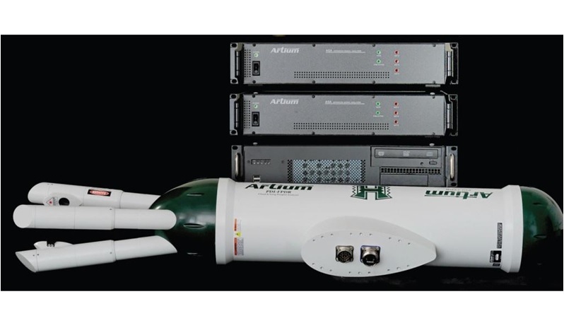
采用美国Artium公司的机载相位多普勒粒子干涉仪(PDI)飞行探头。测量暖积云中微小水液滴的粒径和速度,并据此得出液态水含量LWC数据。探头悬挂安装在双水獭飞机机翼下。在空中飞行状态下,对云层进行测量。
方案详情

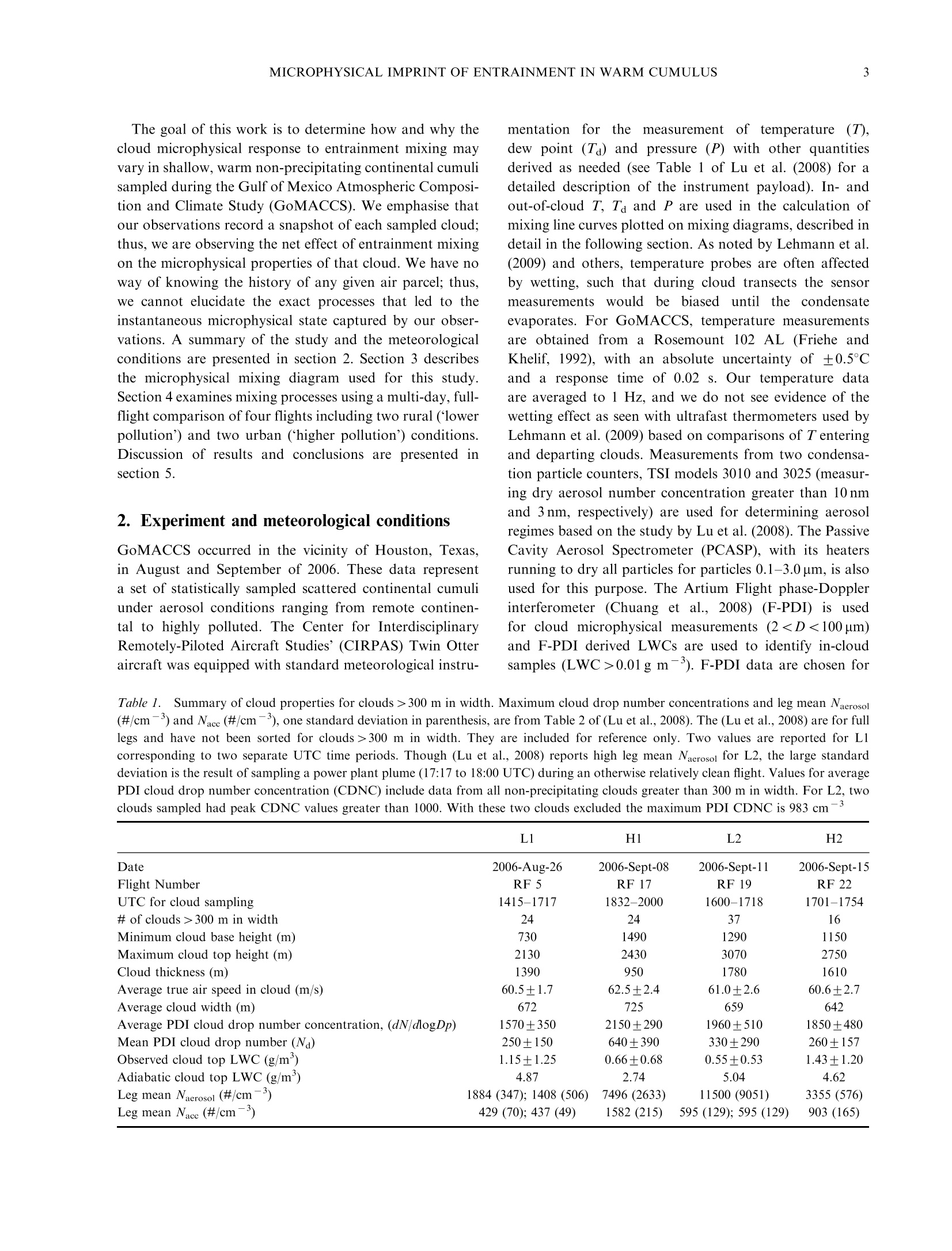
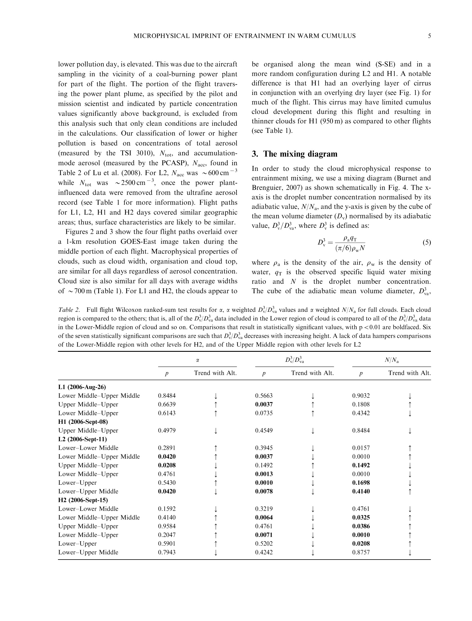
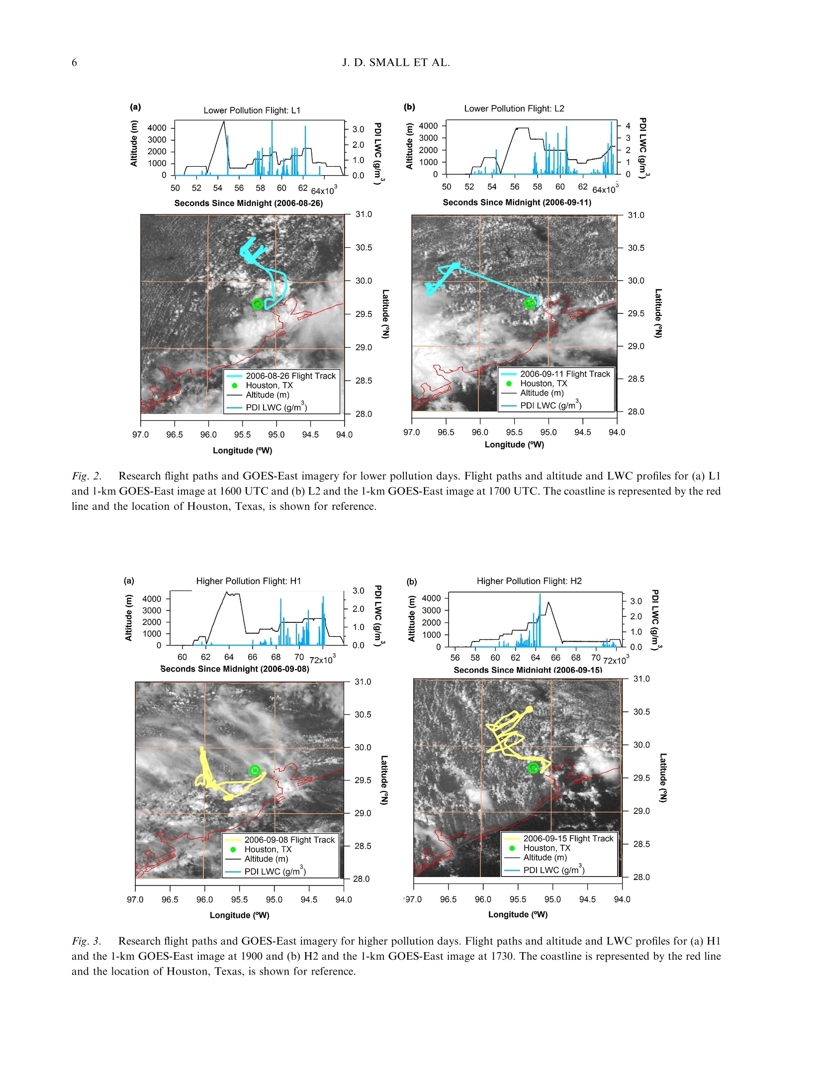
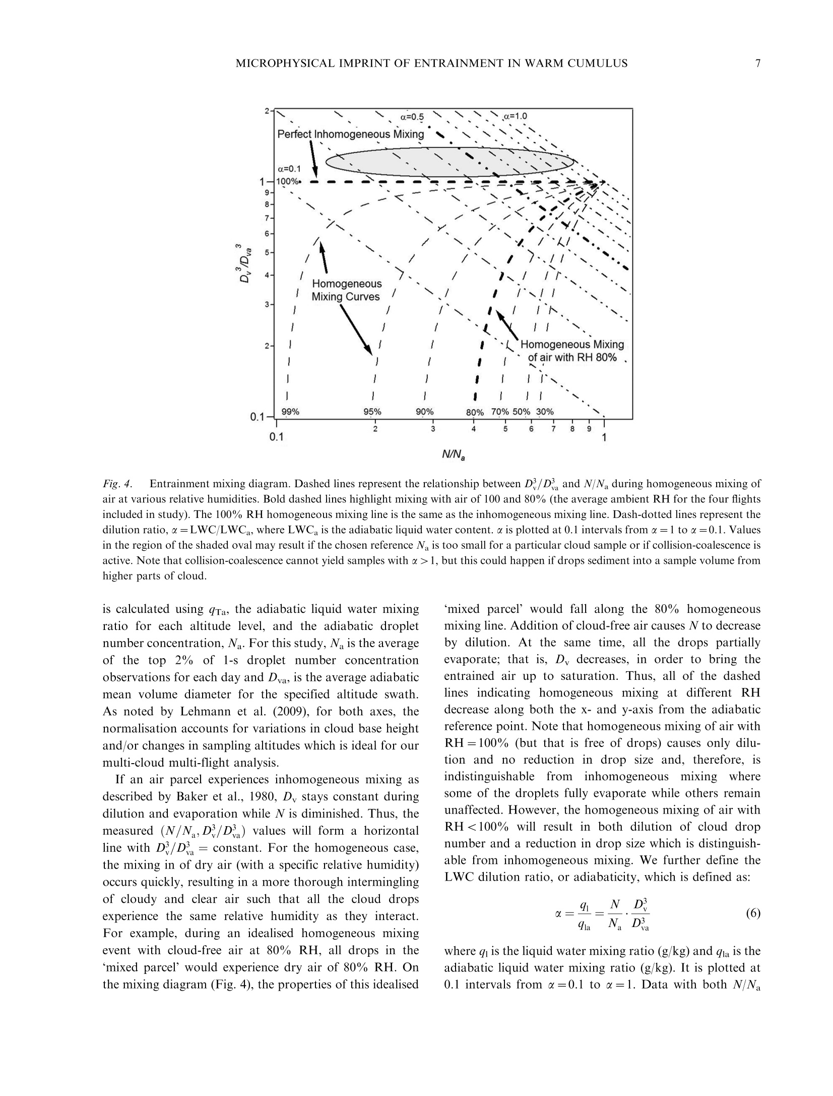
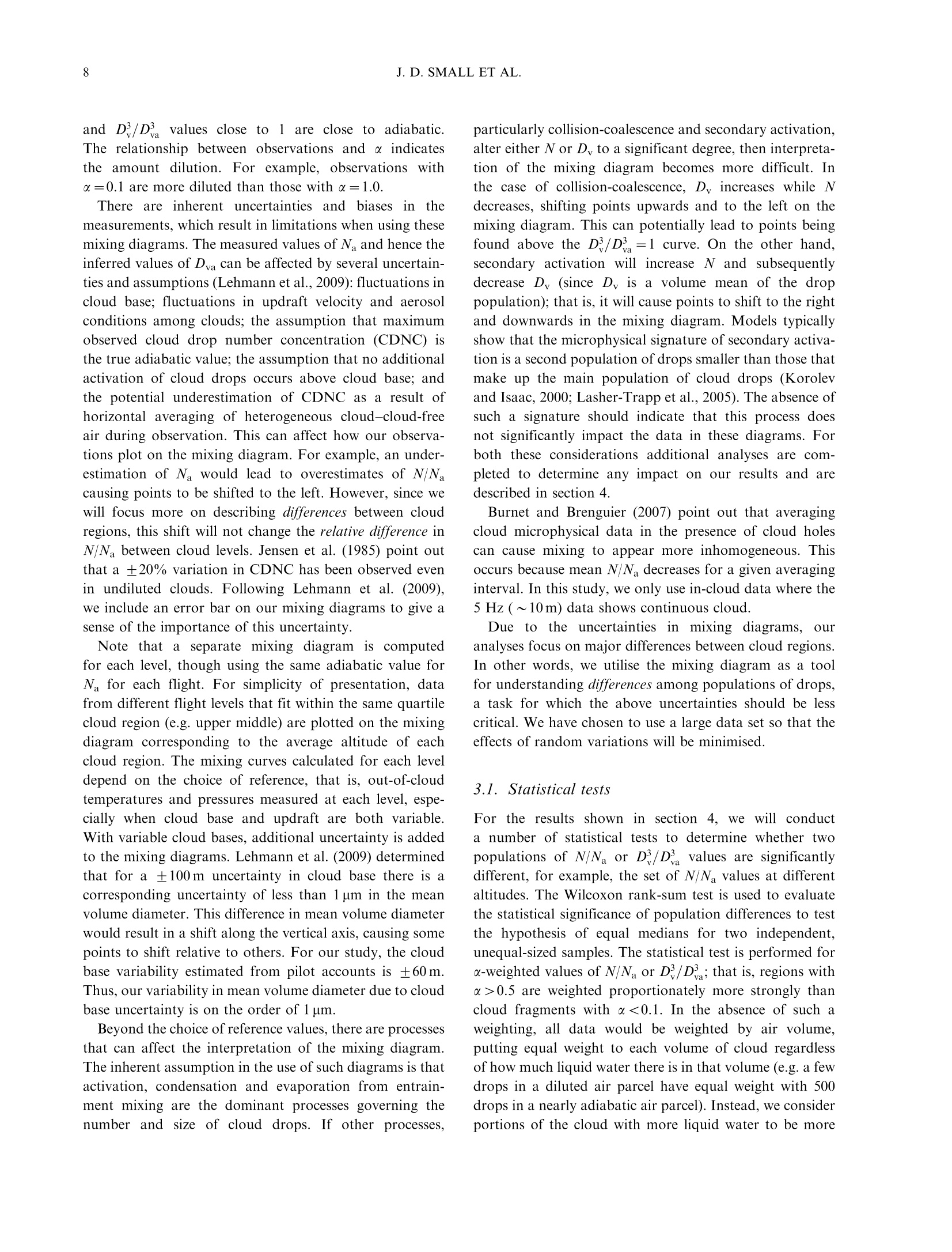
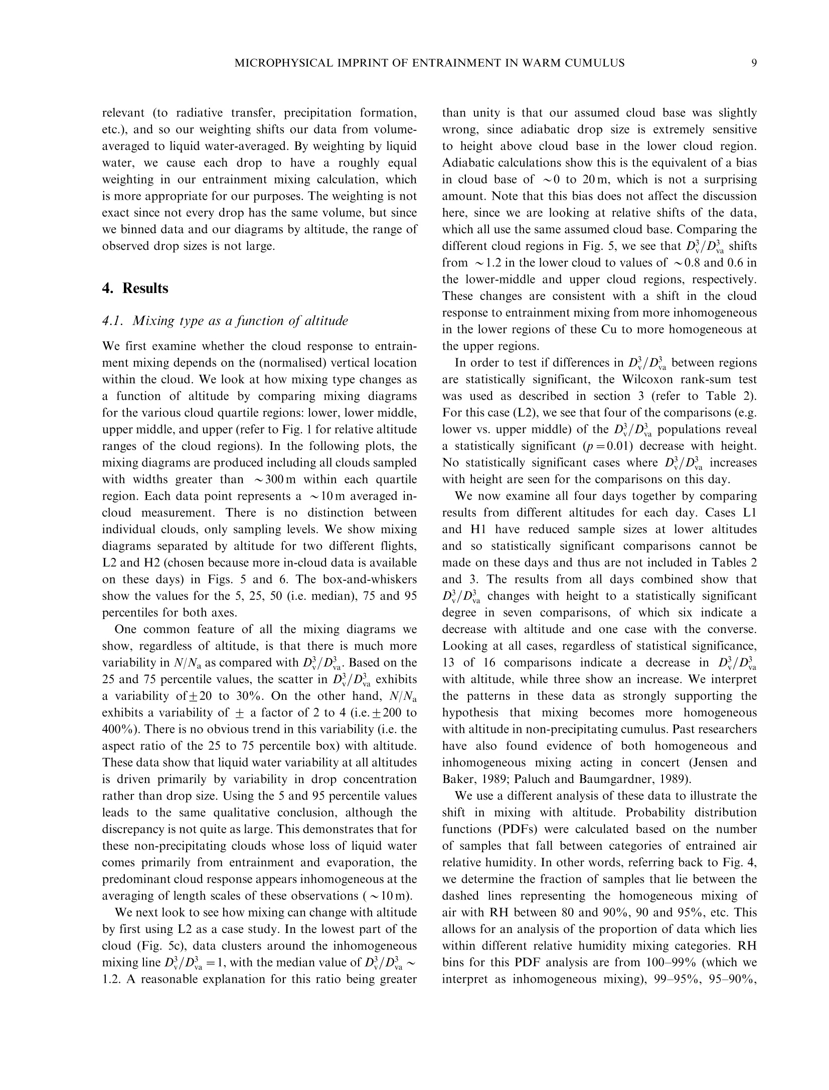
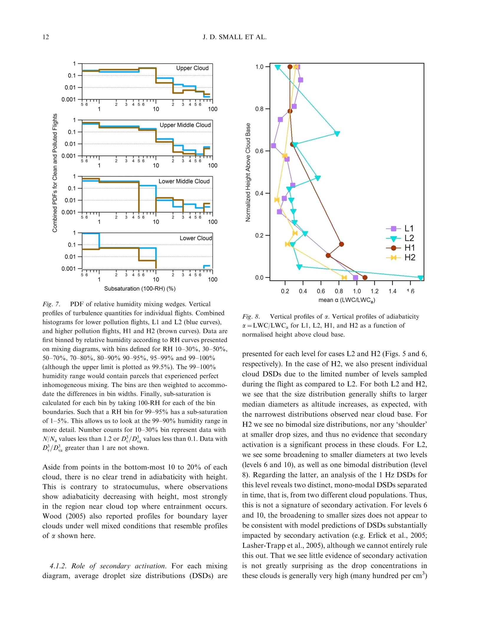
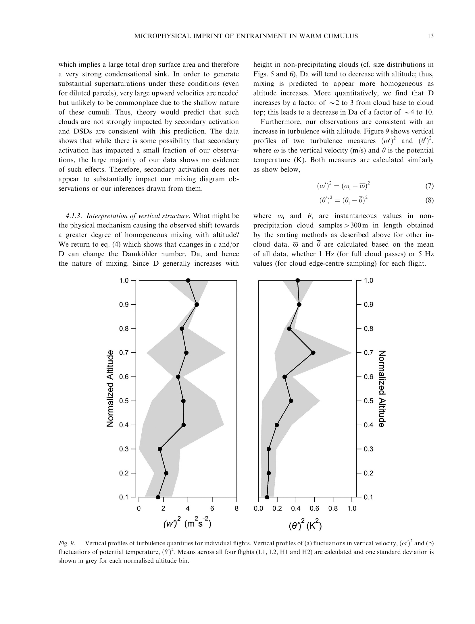
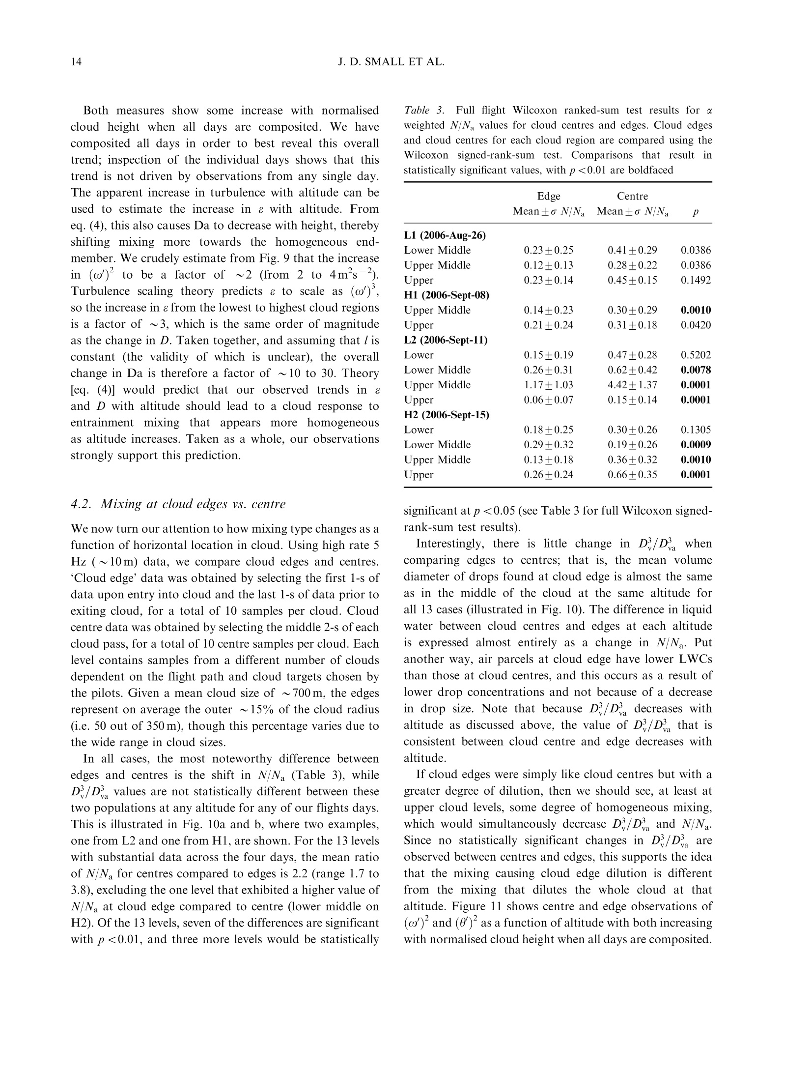
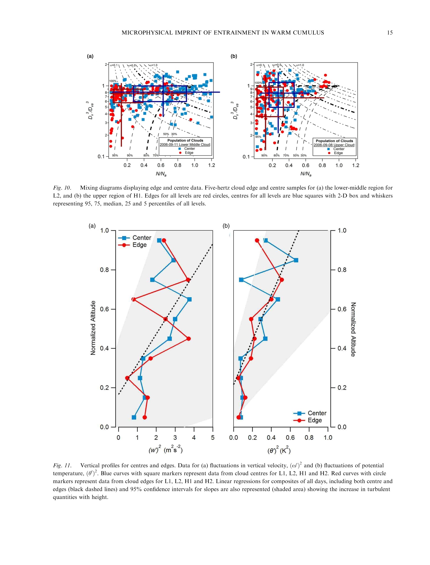
Taylor & FrancisTaylor &Francis GroupTellus B: Chemical and Physical MeteorologyISSN: (Print) 1600-0889 (Online) journal homepage:http://www.tandfonline.com/loi/zelb20 PUBLISHED BY THE INTERNATIONAL METEOROLOGICAL INSTITUTEIN STOCKHOLM Microphysical imprint of entrainment in warmcumulus jennifer D. Small, Patrick Y. Chuang & Haflidi H. jonsson To cite this article: Jennifer D. Small, Patrick Y. Chuang & Haflidi H. Jonsson (2013) Microphysicalimprint of entrainment in warm cumulus, Tellus B: Chemical and Physical Meteorology, 65:1,19922, DOI: 10.3402/tellusb.v65i0.19922 To link to this article: https://doi.org/10.3402/tellusb.v65i0.19922 Published online: 25 jul 2013. Submit your article to this journal C dilAArticle views: 123 Citing articles: 1 View citing articles C http://www.tandfonline.com/action/journalInformation?journalCode=zelb20 Microphysical imprint of entrainment in warm cumulus By JENNIFER D. SMALL, PATRICK Y. CHUANG2* and HAFLIDIH.JONSSON’ ‘Department of Meteorology, University of Hawai'i at Manoa, 2525 Correa Road, Honolulu, HI 96822-2219;Department of Earth and Planetary Sciences, University of California-Santa Cruz, 1156 High Street, Santa Cruz, CA 95064;Center for Interdisciplinary Remotely-Piloted AircraftStudies, Naval Postgraduate School, Monterey, CA 93933 (Manuscript received 19 October 2012; in final form 18 June 2013) ABSTRACT We analyse the cloud microphysical response to entrainment mixing in warm cumulus clouds observed fromthe CIRPAS Twin Otter during the GoMACCS field campaign near Houston, Texas, in summer 2006. Clouddrop size distributions and cloud liquid water contents from the Artium Flight phase-Doppler interferometerin conjunction with meteorological observations are used to investigate the degree to which inhomogeneousversus homogeneous mixing is preferred as a function of height above cloud base, distance from cloud edge andaerosol concentration. Using four complete days of data with 101 cloud penetrations (minimum 300 m inlength), we find that inhomogeneous mixing primarily explains liquid water variability in these clouds.Furthermore, we show that there is a tendency for mixing to be more homogeneous towards the cloud top,which we attribute to the combination of increased turbulent kinetic energy and cloud drop size with altitudewhich together cause the Damkohler number to increase by a factor of between 10 and 30 from cloud base tocloud top. We also find that cloud edges appear to be air from cloud centres that have been diluted solelythrough inhomogeneous mixing. Theory predicts the potential for aerosol to affect mixing type via changes indrop size over the range of aerosol concentrations experienced (moderately polluted rural sites to highlypolluted urban sites). However, the observations, while consistent with this hypothesis, do not show astatistically significant effect of aerosol on mixing type. Keywords: inhomogeneous mixing, homogeneous mixing, GoMACCS, phase-Doppler interferometer, cloudmicrophysics 1. Introduction Entrainment is the process by which sub-saturated airsurrounding a cumulus cloud is drawn into the cloud due tothe (turbulent) motions of the cloudy air. The result ofentrainment is a dilution of both total water and liquidwater, and thus this process is important in governing theevolution of clouds. The mixing of the sub-saturated air with cloudy air, andthe evaporation of liquid water to bring this air to watersaturation, comprise the cloud response to entrainment(hereafter termed entrainment mixing or just mixing).If sufficient dry air is entrained, all the liquid water canevaporate causing complete dissipation of a cloudy volume.If, however, there is an excess of liquid water over thatrequired bringing the entrained air to saturation, then the ( *Corresponding author. ) drop population remaining in the cloud volume has beenaltered due to entrainment. The change in cloud micro-physical properties due to entrainment has been the subjectof numerous studies due to its relevance to key processessuch as precipitation and short-wave reflectance (e.g. Bakeret al., 1980; Paluch and Baumgardner, 1989; Su et al., 1998;Lasher-Trapp et al., 2005; Derkson et al., 2009). In thisstudy, we focus on the following questions relating to themicrophysical response of warm, non-precipitating Cu toentrainment: (1) How does entrainment mixing affect clouddrop size distributions? (2) What does this mixing dependon? and (3) Can aerosol influence the effects of entrainmentmixing? The third question is motivated by interest inthe effects of aerosol on the formation and evolution ofcumulus clouds. Many processes within cumulus clouds depend on theirmicrophysical properties. For example, precipitation andradiative processes depend on the total cloud drop numberconcentration (N) and the mean and shape of the drop size distribution (DSD) for the entire cloud drop popula-tion. Entrainment modifies microphysical properties bydecreasing cloudliquid water content (LWC). SinceLWC~ND, where N is cloud drop concentration andD, is mean volume diameter, the loss of LWC can occur via(1) the decrease of N, termed inhomogeneous mixing (e.g.Latham and Reed, 1977; Hill and Choularton, 1985; Jensenet al., 1985; Lasher-Trapp et al., 2005), (2) a decrease inDy, termed homogeneous mixing (e.g. Baker et al., 1980;Telford et al., 1984; Jensen et al., 1985; Burnet andBrenguier, 2007), or (3) a combination of both, whichrepresents a ‘mixture’of these two end-member types ofmixing (Lasher-Trapp et al., 2005). During homogeneousmixing, after being exposed to sub-saturated air, all dropspartially evaporate to re-establish saturation, causingthe DSD to shift to smaller diameters (the very smallestdrops, a few um in size, may completely evaporate).During inhomogeneous mixing, a subset of drops comple-tely evaporates to re-establish saturation, causing N todecrease, but the shape of the DSD remains the same. Theratio of the time scale it takes for a drop to evaporate, tevap,to the time scale required to mix the cloudy and cloud-freeair, tmix (Baker et al., 1984), is believed to control the cloudmicrophysical response to entrainment, that is, the locationin the continuum between homogeneous and inhomoge-neous mixing. In the limit, homogeneous mixing occurswhen tevap >>Tmix whereby all cloud drops are exposedto the same sub-saturation after complete mixing of thecloud and cloud-free parcels. Perfectly inhomogeneousmixing occurs when the converse is true, that is, tmix>> tevap whereby drops adjacent to sub-saturated regionscompletely evaporate rapidly while the remaining drops arecompletely unaffected. Following Baker et al. (1984), thetime scale for the evaporation of a single drop is given by: where k is a function of temperature and pressure and RHrepresents the relative humidity. We see that Tevap dependson the characteristic drop diameter D. One potentialconsequence is that Tevap will increase with cloud heightas drops grow larger by condensation, all other factors(such as environmental RH and turbulence) being equal.Also, more polluted clouds, with smaller drops, may causetevap to decrease and shift mixing towards the inhomoge-neous end-member (again, all other factors being equal).Lehmann et al. (2009) describe a related time scale, onefor the clear air, without a cloud present, to return tosaturation. This phase-relaxation time scale depends on the rate of evaporation of the entire population of drops,which we re-write as: As LWC increases,Tphase decreases. For fixed LWC,as diameter increases, surface area decreases and thereforetphase increases. Which one of these reaction time scales ismore appropriate depends on the microphysical context,and in some cases when Tphase ~ Tevap, both are smaller thanthe time required to restore saturation (Lehmann et al.,2009). The turbulent mixing time scale is given by: Where I is a mixing length scale and8, the energydissipation rate. Regions of the cloudwith strongerturbulence should have smaller tmix and hence mayshift mixing towards the homogeneous end-member. TheDamkohler number, Da, can be defined as the ratio of themixing time scale to that for phase change, that is: where we have dropped the RH or LWC term for clarity.No matter whether tevap (i.e. single drop) or Tphase (i.e. droppopulation) is used to set the evaporation time scale, thetime scale can be written as proportional to D(althoughthe assumptions are different). If Da is large, inhomoge-neous mixing is favoured, while homogeneous mixingis favoured for smaller Da. Changes in e and/or D are,therefore, predicted to change the nature of mixing inclouds. In reality, the microphysical response to sub-saturatedair is likely to be much more complex. Cumulus clouds arespatially and temporally variable, and mixing occurs acrossa range of scales and changes to the DSD as a result ofmixing are highly variable (Bewley and Lasher-Trapp,2011). Thus no single drop diameter, entrained air relativehumidity, LWC, mixing length scale or energy dissipa-tion rate is likely to be appropriate for computing thesetime scales, even within a single cumulus cloud. Forexample, Lehmann et al. (2009) show that variations in aand Tmix/Tphase by factors as large as 10 and 10, respec-tively, can occur within individual clouds. This suggeststhat mixing can have different character within the samecloud. Some cloudy regions may also have experiencedmultiple dilution events, each potentially of differentcharacter. Lastly, the turbulent transport of cloud dropswill have a tendency to homogenise DSDs within a cloud,such that the signature of a ‘pure'entrainment event wouldbe lost after some time. The goal of this work is to determine how and why thecloud microphysical response to entrainment mixing mayvary in shallow, warm non-precipitating continental cumulisampled during the Gulf of Mexico Atmospheric Composi-tion and Climate Study (GoMACCS). We emphasise thatour observations record a snapshot of each sampled cloud;thus, we are observing the net effect of entrainment mixingon the microphysical properties of that cloud. We have noway of knowing the history of any given air parcel; thus,we cannot elucidate the exact processes that led to theinstantaneous microphysical state captured by our obser-vations. A summary of the study and the meteorologicalconditions are presented in section 2. Section 3 describesthe microphysical mixing diagram used for this study.Section 4 examines mixing processes using a multi-day, full-flight comparison of four flights including two rural (‘lowerpollution’) and two urban (higher pollution’) conditions.Discussion of results and conclusions are presented insection 5. 2. Experiment and meteorological conditions GoMACCS occurred in the vicinity of Houston, Texas,in August and September of 2006. These data representa set of statistically sampled scattered continental cumuliunder aerosol conditions ranging from remote continen-tal to highly polluted. The Center for InterdisciplinaryRemotely-Piloted Aircraft Studies’(CIRPAS) Twin Otteraircraft was equipped with standard meteorological instru- mentation for the measurementof temperature (T),dew point (Ta) and pressure (P) with other quantitiesderived as needed (see Table 1 of Lu et al. (2008) for adetailed description of the instrument payload). In- andout-of-cloud T, Td and P are used in the calculation ofmixing line curves plotted on mixing diagrams, described indetail in the following section. As noted by Lehmann et al.(2009) and others, temperature probes are often affectedby wetting, such that during cloud transects the sensormeasurements wouldlbte biased until the condensateevaporates. For GoMACCS, temperature measurementsare obtained from a Rosemount 102 AL (Friehe andKhelif, 1992), with an absolute uncertainty of±0.5℃and a response time of 0.02 s. Our temperature dataare averaged to 1 Hz, and we do not see evidence of thewetting effect as seen with ultrafast thermometers used byLehmann et al.(2009) based on comparisons of T enteringand departing clouds. Measurements from two condensa-tion particle counters, TSI models 3010 and 3025 (measur-ing dry aerosol number concentration greater than 10 nmand 3 nm, respectively) are used for determining aerosolregimes based on the study by Lu et al. (2008). The PassiveCavity Aerosol Spectrometer (PCASP), with its heatersrunning to dry all particles for particles 0.1-3.0 um, is alsoused for this purpose. The Artium Flight phase-Dopplerinterferometer (Chuang et al., 2008) (F-PDI) iss usedfor cloud microphysical measurements (20.01g m-3). F-PDI data are chosen for Tablee 1I. Summary of cloud properties for clouds>300 m in width. Maximum cloud drop number concentrations and leg mean Naerosol(#/cm-) and Nacc (#/cm-3), one standard deviation in parenthesis, are from Table 2 of (Lu et al., 2008). The (Lu et al., 2008) are for fulllegs and have not been sorted for clouds >300 m in width. They are included for reference only. Two values are reported for L1corresponding to two separate UTC time periods. Though (Lu et al., 2008) reports high leg mean Naerosol for L2, the large standarddeviation is the result of sampling a power plant plume (17:17 to 18:00 UTC) during an otherwise relatively clean flight. Values for averagePDI cloud drop number concentration (CDNC) include data from all non-precipitating clouds greater than 300 m in width. For L2, twoclouds sampled had peak CDNC values greater than 1000. With these two clouds excluded the maximum PDI CDNC is 983 cm-' L1 H1 L2 H2 Date 2006-Aug-26 2006-Sept-08 2006-Sept-11 2006-Sept-15 Flight Number RF 5 RF 17 RF 19 RF 22 UTC for cloud sampling 1415-1717 1832-2000 1600-1718 1701-1754 # of clouds > 300 m in width 24 24 37 16 Minimum cloud base height (m) 730 1490 1290 1150 Maximum cloud top height (m) 2130 2430 3070 2750 Cloud thickness (m) 1390 950 1780 1610 Average true air speed in cloud (m/s) 60.5±1.7 62.5±2.4 61.0±2.6 60.6±2.7 Average cloud width (m) 672 725 659 642 Average PDI cloud drop number concentration,(dN/dlogDp) 1570±350 2150±290 1960+510 1850±480 Mean PDI cloud drop number (Na) 250+150 640±390 330+290 260±157 Observed cloud top LWC (g/m) 1.15±1.25 0.66±0.68 0.55+0.53 1.43±1.20 Adiabatic cloud top LWC (g/m’) 4.87 2.74 5.04 4.62 Leg mean Naerosol (#/cm) 1884 (347);1408 (506) 7496 (2633) 11500(9051) 3355 (576) Leg mean Nacc (#/cm) 429(70);437 (49) 1582(215) 595 (129);595(129) 903(165) in-cloud identification due to the ability of the F-PDIto detect large numbers of cloud droplets without coin-cidence effects (see Chuang et al., 2008 for a more detaileddescription of F-PDIlimitations andcapabilities).A combination of F-PDI and data from the Cloud Imag-ing Probe (CIP) component of the Cloud, Aerosol andPrecipitation Spectrometer Probe (Baumgardner et al.(2001),1550 um) and limit our analysis to non-precipitatingclouds. Soundings of T, Ta and RH taken during clear-air spiralsbefore or after cloud sampling on the four days used in thisstudy are shown in Fig. 1 along with the average height ofcloud base and cloud top for each flight. Cloud base andcloud top heights are defined as the lowest level and highestlevel at which clouds were sampled for each day, as de-scribed by CIRPAS pilots and the on-board mission scien-tist. During any particular flight cloud base remained fairlyconstant varying, on average, by ±60 m based on pilotaccounts. We report altitude-dependent results using fourdifferent cloud regions, denoted lower,lower middle, uppermiddle, and upper. These quartile regions are determinedas the bottom 25%, 25-50%,50-75% and upper 25% ofaltitudes for each flight, as illustrated in Fig. 1, regardlessof their absolute altitude. Use of normalised cloud heightis common for comparison among different cloud cases(Jiang et al., 2006; Lu et al., 2008; Small et al., 2009). We note that on any given day, cloud penetrations arenot evenly distributed among these different levels, and onsome days, there may be no data at all from one region (e.g.lower middle) while another region was very well sampled. 2.1. Statistical sampling of cumulus fields For this study we choose to use two lower pollution flights,denoted L1 (2006-Aug-26) and L2 (2006-Sept-11) and twohigher pollution flights denoted H1 (2006-Sept-08) and H2(2006-Sept-15) out of the 22 GoMACCS research flights.For each flight, sampling of cumulus fields occurred byselecting closest reasonable cloud targets such that the dataconsists of an unbiased sample of cloud microphysical anddynamical properties over a large geographic region undersimilar meteorological conditions. We choose the twomost-polluted and two least-polluted flights, with satisfac-tory cloud sampling, in order to maximise the aerosolconcentration contrast. All flight data have been filteredsuch that only non-precipitating cumulus are included inthe analysis. Filtering is critical since the mixing diagram ismost useful under conditions of minimal collision-coales-cence as discussed below. We also filter for clouds greaterthan 300 m in width. Over all flights, mean and o of cloudwidth are 680 and 337m, respectively. Detailed informationregarding each flight is available in Table 1. Note that theultrafine aerosol concentration during L2, classified as a Fig. I. Out-of-cloud atmospheric soundings. Vertical soundings for four full flights L1 (2006-Aug-26), L2 (2006-Sept-11), H1 (2006-Sept-08) and H2 (2006-Sept-15). Note that RH measurement problems occurred during large portions of the sounding for H2 (i.e. valuesabove 100%). Grey shaded areas represent cloud layers (from lowest observed cloud base to highest observed cloud top) for each researchflight. Approximate altitudes for cloud regions, lower (L), lower middle (LM), upper middle (UM) and upper (U) for each flight areseparated by dotted lines. lower pollution day, is elevated. This was due to the aircraftsampling in the vicinity of a coal-burning power plantfor part of the flight. The portion of the flight travers-ing the power plant plume, as specified by the pilot andmission scientist and indicated by particle concentrationvalues significantly above background, is excluded fromthis analysis such that only clean conditions are includedin the calculations. Our classification of lower or higherpollution is, based on concentrations of total aerosol(measured by the TSI 3010), Ntot, and accumulation-mode aerosol (measured by the PCASP), Nacc, found inTable 2 of Lu et al. (2008). For L2, Nace was ~600cmwhile Ntotwas ~2500cm-3, once the power plant-influenced data were removed from the ultrafine aerosolrecord (see Table 1 for more information). Flight pathsfor L1, L2, H1 and H2 days covered similar geographicareas; thus, surface characteristics are likely to be similar. Figures 2 and 3 show the four flight paths overlaid over a 1-km resolution GOES-East image taken during the middle portion of each flight. Macrophysical properties of clouds, such as cloud width, organisation and cloud top, are similar for all days regardless of aerosol concentration. Cloud size is also similar for all days with average widths of ~700 m (Table 1). For L1 and H2, the clouds appear to be organised along the mean wind (S-SE) and in amore random configuration during L2 and H1. A notabledifference is that H1 had an overlying layer of cirrusin conjunction with an overlying dry layer (see Fig.1) formuch of the flight. This cirrus may have limited cumuluscloud development during this flight and resulting inthinner clouds for H1 (950 m) as compared to other flights(see Table 1). 3. The mixing diagram In order to study the cloud microphysical response toentrainment mixing, we use a mixing diagram (Burnet andBrenguier, 2007) as shown schematically in Fig. 4. The x-axis is the droplet number concentration normalised by itsadiabatic value, N/Na, and the y-axis is given by the cube ofthe mean volume diameter (D) normalised by its adiabaticvalue, D/Das where D is defined as: where Pa is the density ofthe air, pw is the density ofwater, 9r is the observed specific liquid water mixingratio andNis the droplet number concentration.The cube of the adiabatic mean volume diameter, Da Table 2. Full flight Wilcoxon ranked-sum test results for a, a weighted D/Da values and o weighted N/N for full clouds. Each cloudregion is compared to the others; that is, all of the D/Da data included in the Lower region of cloud is compared to all of the D/Dva datain the Lower-Middle region of cloud and so on. Comparisons that result in statistically significant values, with p <0.01 are boldfaced. Sixof the seven statistically significant comparisons are such that D/Dia decreases with increasing height. A lack of data hampers comparisonsof the Lower-Middle region with other levels for H2, and of the Upper Middle region with other levels for L2 D/D N/Na p Trend with Alt. Trend with Alt. Trend with Alt. L1 (2006-Aug-26) Lower Middle-Upper Middle 0.8484 0.5663 0.9032 Upper Middle-Upper 0.6639 0.0037 0.1808 Lower Middle-Upper 0.6143 0.0735 0.4342 H1 (2006-Sept-08) Upper Middle-Upper 0.4979 0.4549 0.8484 L2 (2006-Sept-11) Lower-Lower Middle 0.2891 0.3945 0.0157 Lower Middle-Upper Middle 0.0420 0.0037 0.0010 Upper Middle-Upper 0.0208 0.1492 0.1492 Lower Middle-Upper 0.4761 0.0013 0.0010 Lower-Upper 0.5430 0.0010 0.1698 Lower-Upper Middle 0.0420 0.0078 0.4140 H2 (2006-Sept-15) Lower-Lower Middle 0.1592 0.3219 0.4761 Lower Middle-Upper Middle 0.4140 0.0064 0.0325 Upper Middle-Upper 0.9584 0.4761 0.0386 Lower Middle-Upper 0.2047 0.0071 0.0010 Lower-Upper 0.5901 0.5202 0.0208 Lower-Upper Middle 0.7943 0.4242 0.8757 Fig. 2. Research flight paths and GOES-East imagery for lower pollution days. Flight paths and altitude and LWC profiles for (a) L1and 1-km GOES-East image at 1600 UTC and(b) L2 and the 1-km GOES-East image at 1700 UTC. The coastline is represented by the redline and the location of Houston, Texas, is shown for reference. ata Fig. 3. Research flight paths and GOES-East imagery for higher pollution days. Flight paths and altitude and LWC profiles for (a) H1and the 1-km GOES-East image at 1900 and (b) H2 and the 1-km GOES-East image at 1730. The coastline is represented by the red lineand the location of Houston, Texas, is shown for reference. N/N. Fig.4. Entrainment mixing diagram. Dashed lines represent the relationship between D/Dia and N/N during homogeneous mixing ofair at various relative humidities. Bold dashed lines highlight mixing with air of 100 and 80% (the average ambient RH for the four flightsincluded in study). The 100% RH homogeneous mixing line is the same as the inhomogeneous mixing line. Dash-dotted lines represent thedilution ratio,α=LWC/LWCa, where LWCa is the adiabatic liquid water content. a is plotted at 0.1 intervals from =1 to α=0.1. Valuesin the region of the shaded oval may result if the chosen reference Na is too small for a particular cloud sample or if collision-coalescence isactive. Note that collision-coalescence cannot yield samples with a>1, but this could happen if drops sediment into a sample volume fromhigher parts of cloud. is calculated using gTa, the adiabatic liquid water mixingratio for each altitude level, and the adiabatic dropletnumber concentration,Na. For this study, Na is the averageof the top 2% of 1-s droplet number concentrationobservations for each day and Dva, is the average adiabaticmean volume diameter for the specified altitude swath.As noted by Lehmann et al. (2009), for both axes, thenormalisation accounts for variations in cloud base heightand/or changes in sampling altitudes which is ideal for ourmulti-cloud multi-flight analysis. If an air parcel experiences inhomogeneous mixing asdescribed by Baker et al., 1980, D, stays constant duringdilution and evaporation while N is diminished. Thus, themeasured (N/N,D/D) values will form a horizontalline with D:/Da= constant. For the homogeneous case,the mixing in of dry air (with a specific relative humidity)occurs quickly, resulting in a more thorough interminglingof cloudy and clear air such that all the cloud dropsexperience the same relative humidity as they interact.For example, during an idealised homogeneous mixingevent with cloud-free air at 80% RH, all drops in the‘mixed parcel’would experience dry air of 80% RH. Onthe mixing diagram (Fig. 4), the properties of this idealised ‘mixed parcel would fall along the 80% homogeneousmixing line. Addition of cloud-free air causes N to decreaseby dilution. At the same time, all the drops partiallyevaporate; that is, D, decreases, in order to bring theentrained air up to saturation. Thus, all of the dashedlines indicating homogeneous mixing at different RHdecrease along both the x- and y-axis from the adiabaticreference point. Note that homogeneous mixing of air withRH=100% (but that is free of drops) causes only dilu-tion and no reduction in drop size and, therefore, isindistinguishable from11inhomogeneous mixingwheresome of the droplets fully evaporate while others remainunaffected. However, the homogeneous mixing of air withRH<100% will result in both dilution of cloud dropnumber and a reduction in drop size which is distinguish-able from inhomogeneous mixing. We further define theLWC dilution ratio, or adiabaticity, which is defined as: where q is the liquid water mixing ratio (g/kg) and qia is theadiabatic liquid water mixing ratio (g/kg). It is plotted at0.1 intervals from a=0.1 to α=1. Data with both N/N. and Di/Dia values close to 1 are close to adiabatic.The relationship between observations and a indicatesthe amount dilution. For example, observations witho=0.1 are more diluted than those withα=1.0. There are inherent uncertainties and biases in themeasurements, which result in limitations when using thesemixing diagrams. The measured values of Na and hence theinferred values of Dva can be affected by several uncertain-ties and assumptions (Lehmann et al., 2009): fluctuations incloud base; fluctuations in updraft velocity and aerosolconditions among clouds; the assumption that maximumobserved cloud drop number concentration (CDNC) isthe true adiabatic value; the assumption that no additionalactivation of cloud drops occurs above cloud base; andthe potential underestimation of CDNC as a result ofhorizontal averaging of heterogeneous cloud-cloud-freeair during observation. This can affect how our observa-tions plot on the mixing diagram. For example, an under-estimation of Na would lead to overestimates of N/Nacausing points to be shifted to the left. However, since wewill focus more on describing differences between cloudregions, this shift will not change the relative difference inN/Na between cloud levels. Jensen et al. (1985) point outthat a +20% variation in CDNC has been observed evenin undiluted clouds. Following Lehmann et al. (2009),we include an error bar on our mixing diagrams to give asense of the importance of this uncertainty. Note that a separate mixing diagram is computedfor each level, though using the same adiabatic value forNa for each flight. For simplicity of presentation, datafrom different flight levels that fit within the same quartilecloud region (e.g. upper middle) are plotted on the mixingdiagram corresponding to the average altitude of eachcloud region. The mixing curves calculated for each leveldepend on the choice of reference, that is, out-of-cloudtemperatures and pressures measured at each level, espe-cially when cloud base and updraft are both variable.With variable cloud bases, additional uncertainty is addedto the mixing diagrams. Lehmann et al. (2009) determinedthat for a±100m uncertainty in cloud base there is acorresponding uncertainty of less than 1 um in the meanvolume diameter. This difference in mean volume diameterwould result in a shift along the vertical axis, causing somepoints to shift relative to others. For our study, the cloudbase variability estimated from pilot accounts is ±60 m.Thus, our variability in mean volume diameter due to cloudbase uncertainty is on the order of 1 um. Beyond the choice of reference values, there are processesthat can affect the interpretation of the mixing diagram.The inherent assumption in the use of such diagrams is thatactivation, condensation and evaporation from entrain-ment mixing are the dominant processes governing thenumber and size of cloud drops. If other processes, particularly collision-coalescence and secondary activation,alter either N or Dy to a significant degree, then interpreta-tion of the mixing diagram becomes more difficult. Inthe case of collision-coalescence, D, increases while Ndecreases, shifting points upwards and to the left on themixing diagram. This can potentially lead to points beingfound above the D:/Da=1 curve. On the other hand,secondary activation will increase N and subsequentlydecrease Dv (since D, is a volume mean of the droppopulation); that is, it will cause points to shift to the rightand downwards in the mixing diagram. Models typicallyshow that the microphysical signature of secondary activa-tion is a second population of drops smaller than those thatmake up the main population of cloud drops (Korolevand Isaac, 2000; Lasher-Trapp et al., 2005). The absence ofsuch a signature should indicate that this process doesnot significantly impact the data in these diagrams. Forboth these considerations additional analyses are com-pleted to determine any impact on our results and aredescribed in section 4. Burnet and Brenguier (2007) point out that averagingcloud microphysical data in the presence of cloud holescan cause mixing to appear more inhomogeneous. Thisoccurs because mean N/Na decreases for a given averaginginterval. In this study, we only use in-cloud data where the5 Hz (~10m) data shows continuous cloud. Due to the uncertainties in mixing diagrams, ouranalyses focus on major differences between cloud regions.In other words, we utilise the mixing diagram as a toolfor understanding differences among populations of drops,a task for which the above uncertainties should be lesscritical. We have chosen to use a large data set so that theeffects of random variations will be minimised. 3.1. Statistical tests For the results shown in section 4, we will conducta number of statistical tests to determine whether twopopulations of N/Na or D/Davalues are significantlydifferent, for example, the set of N/Na values at differentaltitudes. The Wilcoxon rank-sum test is used to evaluatethe statistical significance of population differences to testthe hypothesis of equal medians for two independent,unequal-sized samples. The statistical test is performed foru-weighted values of N/Na or D/Da; that is, regions withα>0.5 are weighted proportionately more strongly thancloud fragments with α<0.1. In the absence of such aweighting, all data would be weighted by air volume,putting equal weight to each volume of cloud regardlessof how much liquid water there is in that volume (e.g. a fewdrops in a diluted air parcel have equal weight with 500drops in a nearly adiabatic air parcel). Instead, we considerportions of the cloud with more liquid water to be more relevant (to radiative transfer, precipitation formation,etc.), and so our weighting shifts our data from volume-averaged to liquid water-averaged. By weighting by liquidwater, we cause each drop to have a roughly equalweighting in our entrainment mixing calculation, whichis more appropriate for our purposes. The weighting is notexact since not every drop has the same volume, but sincewe binned data and our diagrams by altitude, the range ofobserved drop sizes is not large. 4. Results 4.1. Mixing type as a function of altitude We first examine whether the cloud response to entrain-ment mixing depends on the (normalised) vertical locationwithin the cloud. We look at how mixing type changes asa function of altitude by comparing mixing diagramsfor the various cloud quartile regions: lower, lower middle,upper middle,and upper (refer to Fig. 1 for relative altituderanges of the cloud regions). In the following plots, themixing diagrams are produced including all clouds sampledwith widths greater than ~300 m within each quartileregion. Each data point represents a ~10m averaged in-cloud measurement. There is no (distinction betweenindividual clouds, only sampling levels. We show mixingdiagrams separated by altitude for two different flights,L2 and H2 (chosen because more in-cloud data is availableon these days) in Figs. 5 and 6. The box-and-whiskersshow the values for the 5, 25, 50 (i.e. median), 75 and 95percentiles for both axes. One common feature of all the mixing diagrams weshow, regardless of altitude, is that there is much morevariability in N/Na as compared with D/D. Based on the25 and 75 percentile values, the scatter in D:/D? exhibitsa variability of±20 to 30%. On the other hand, N/Naexhibits a variability of ± a factor of 2 to 4 (i.e.±200 to400%). There is no obvious trend in this variability (i.e. theaspect ratio of the 25 to 75 percentile box) with altitude.These data show that liquid water variability at all altitudesis driven primarily by variability in drop concentrationrather than drop size. Using the 5 and 95 percentile valuesleads to the same qualitative conclusion, although thediscrepancy is not quite as large. This demonstrates that forthese non-precipitating clouds whose loss of liquid watercomes primarily from entrainment and evaporation, thepredominant cloud response appears inhomogeneous at theaveraging of length scales of these observations (~10m). We next look to see how mixing can change with altitudeby first using L2 as a case study. In the lowest part of thecloud (Fig. 5c), data clusters around the inhomogeneousmixing line D:/Da=1, with the median value of D:/Da~1.2. A reasonable explanation for this ratio being greater than unity is that our assumed cloud base was sightlywrong, since adiabatic drop size is extremely sensitiveto height above cloud base in the lower cloud region.Adiabatic calculations show this is the equivalent of a biasin cloud base of ~0 to 20 m, which is not a surprisingamount. Note that this bias does not affect the discussionhere, since we are looking at relative shifts of the data,which all use the same assumed cloud base. Comparing thedifferent cloud regions in Fig. 5, we see that D./Da shiftsfrom ~1.2 in the lower cloud to values of ~0.8 and 0.6 inthe lower-middle and upper cloud regions, respectively.These changes are consistent with a shift in the cloudresponse to entrainment mixing from more inhomogeneousin the lower regions of these Cu to more homogeneous atthe upper regions. In order to test if differences in D./D between regionsare statistically significant, the Wilcoxon rank-sum testwas used as described in section 3 (refer to Table 2).For this case (L2), we see that four of the comparisons (e.g.lower vs. upper middle) of the D/D populations reveala statistically significant (p=0.01) decrease with height.No statistically significant cases where D/Da increaseswith height are seen for the comparisons on this day. We now examine all four days together by comparingresults from different altitudes for each day. Cases L1and H1 lhave reduced sample sizes at lower altitudesandd so statistically significant comparisons cannot bemade on these days and thus are not included in Tables 2and 3. The results from all days combined show thatD/Da changes with height to a statistically significantdegree in seven comparisons, of which six indicate adecrease with altitude and one case with the converse.Looking at all cases, regardless of statistical significance,13 of 16 comparisons indicate a decrease in D/Dwith altitude, while three show an increase. We interpretthe patterns in these data as strongly supporting thehypothesis1Sthat mixing becomes more lhomogeneouswith altitude in non-precipitating cumulus. Past researchershave also found evidence of both homogeneous andinhomogeneous mixing acting in concert (Jensen andBaker, 1989; Paluch and Baumgardner, 1989). We use a different analysis of these data to illustrate theshift in mixinggwith altitude. Probability distributionfunctions (PDFs) were calculated based on the numberof samples that fall between categories of entrained airrelative humidity. In other words, referring back to Fig. 4,we determine the fraction of samples that lie between thedashed lines representing the homogeneous mixing ofair with RH between 80 and 90%,90 and 95%, etc. Thisallows for an analysis of the proportion of data which lieswithin different relative humidity mixing categories. RHbins for this PDF analysis are from 100-99% (which weinterpret as inhomogeneous mixing), 99-95%, 95-90%, Fig. 5. 1-Hz data plotted as a function of altitude and corresponding average DSD for each level (coloured markers and lines based onaltitude) for (a) upper cloud, (b) lower-middle cloud and (c) lower cloud with 2-D box and whiskers representing 95, 75, median, 25 and 5percentiles of all levels. 90-80%,80-70%,70-50% and 50-30%. Note that Fig. 7is plotted with the y-axis as sub-saturation for clarity athigh RH, so 80-90% RH is plotted as 10-20% sub-saturation. Data with N/Na or D/Dva values greater than1.2 or less than 0.1 were excluded. A parcel of air whosedrops have experienced a mixture of homogeneous andinhomogeneous mixing will appear on the mixing diagramas having experienced one single homogeneous mixingevent, but at a higher RH than was actually encountered.One can see this by following a line of constant adiabaticity in the sample mixing diagram in Fig. 4. The PDFs inFig. 7 show that as height above cloud base increases, thenumber of samples that plot in lower relative humiditywedges’ increases. This is evident in both the lower andthe higher pollution examples. This different approach toanalysing the data further supports the hypothesis thathomogeneous mixing becomes more important at higherlevels in a cloud. Looking at variations in N/Na there is no statisticallysignificant difference when comparing vertical cloud regions Fig. 6. 1-Hz data plotted as a function of altitude (coloured markers) and corresponding average DSD foreach level and individualclouds (coloured lines based on altitude) for (a) upper cloud,(b) upper-middle cloud and (c) lower cloud with 2-D box and whiskersrepresenting 95, 75, median, 25 and 5 percentiles of all levels. and no observed trend in N/Nwith increased altitude,which is consistent with inspection of Figs. 5 and 6. It must be noted that the points on the mixing diagramsfor the chosen layers often do not appear to fall‘perfectly'along the homogeneous mixing lines and there is muchscatter. This is due in part to the large number of samplesand different clouds at each level. Another considerationis that aircraft observations provide only instantaneousobservations and it is not possible to know the mixinghistory of any given sample. 4.1.1. Adiabaticity profiles. Adiabaticity a can also becompared among different cloud altitude regions. Table 2shows that of the 16 available comparisons, only three arestatistically significant, with two of the three supportingan increase in a with height. Nine of 16 comparisonsindicate an increase in a with cloud height, and the otherseven indicate a decrease. These data thus support a null-hypothesis adiabaticity profile where there’s no clearchange with altitude. To support this point, vertical profilesof o are plotted in Fig. 8 following Fig. 4c of Wood (2005). Fig. 7. PDF of relative humidity mixing wedges. Vertical profiles of turbulence quantities for individual flights. Combinedhistograms for lower pollution flights, L1 and L2 (blue curves),and higher pollution flights, H1 and H2 (brown curves). Data arefirst binned by relative humidity according to RH curves presentedon mixing diagrams, with bins defined for RH 10-30%,30-50%,50-70%,70-80%,80-90%90-95%,95-99% and 99-100%(although the upper limit is plotted as 99.5%). The 99-100%humidity range would contain parcels that experienced perfectinhomogeneous mixing. The bins are then weighted to accommo-date the differences in bin widths. Finally, sub-saturation iscalculated for each bin by taking 100-RH for each of the binboundaries. Such that a RH bin for 99-95% has a sub-saturationof 1-5%. This allows us to look at the 99-90% humidity range inmore detail. Number counts for 10-30% bin represent data withN/Na values less than 1.2 or D/D values less than 0.1. Data withD/Dgreater than 1 are not shown. Aside from points in the bottom-most 10 to 20% of eachcloud, there is no clear trend in adiabaticity with height.This is contrary to stratocumulus, where observationsshow adiabaticity decreasing with height, most stronglyin the region near cloud top where entrainment occurs.Wood (2005) also reported profiles for boundary layerclouds under well mixed conditions that resemble profilesof a shown here. 4.1.2. Role of secondary activation. For each mixingdiagram, average droplet size distributions (DSDs) are Fig. 8. Vertical profiles of o. Vertical profiles of adiabaticitya=LWC/LWCa for L1, L2, H1, and H2 as a function ofnormalised height above cloud base. presented for each level for cases L2 and H2 (Figs. 5 and 6,respectively). In the case of H2, we also present individualcloud DSDs due to the limited number of levels sampledduring the flight as compared to L2. For both L2 and H2,we see that the size distribution generally shifts to largermedian diameters as altitude increases, as expected, withthe narrowest distributions observed near cloud base. ForH2 we see no bimodal size distributions, nor any shoulder’at smaller drop sizes, and thus no evidence that secondaryactivation is a significant process in these clouds. For L2,we see some broadening to smaller diameters at two levels(levels 6 and 10), as well as one bimodal distribution (level8). Regarding the latter, an analysis of the 1 Hz DSDs forthis level reveals two distinct,mono-modal DSDs separatedin time, that is, from two different cloud populations. Thus,this is not a signature of secondary activation. For levels 6and 10, the broadening to smaller sizes does not appear tobe consistent with model predictions of DSDs substantiallyimpacted by secondary activation (e.g. Erlick et al., 2005;Lasher-Trapp et al., 2005), although we cannot entirely rulethis out. That we see little evidence of secondary activationis not greatly surprising as the drop concentrations inthese clouds is generally very high (many hundred per cm’) which implies a large total drop surface area and thereforea very strong condensational sink. In order to generatesubstantial supersaturations under these conditions (evenfor diluted parcels), very large upward velocities are neededbut unlikely to be commonplace due to the shallow natureof these cumuli. Thus, theory would predict that suchclouds are not strongly impacted by secondary activationand DSDs are consistent with this prediction. The datashows that while there is some possibility that secondaryactivation has impacted a small fraction of our observa-tions, the large majority of our data shows no evidenceof such effects. Therefore, secondary activation does notappear to substantially impact our mixing diagram ob-servations or our inferences drawn from them. height in non-precipitating clouds (cf. size distributions inFigs. 5 and 6), Da will tend to decrease with altitude; thus,mixing is predicted to appear more homogeneous asaltitude increases. More quantitatively, we find that Dincreases by a factor of ~2 to 3 from cloud base to cloudtop; this leads to a decrease in Da of a factor of ~4 to 10. Furthermore, our observations are consistent with anincrease in turbulence with altitude. Figure 9 shows verticalprofiles o01f two turbulence measures (ω)’ and (0),where ω is the vertical velocity (m/s) and 0 is the potentialtemperature (K). Both measures are calculated similarlyas show below, (ω)=(ω-) (7) 4.1.3. Interpretation ofvertical structure. What might bethe physical mechanism causing the observed shift towardsa greater degree of homogeneous mixing with altitude?We return to eq. (4) which shows that changes in e and/orD can change the Damkohler number, Da, and hencethe nature of mixing. Since D generally increases with where ω and 0; areeinstantaneousvalues innon-precipitation cloud samples>300 m in length obtainedby the sorting methods as described above for other in-cloud data. w and 0 are calculated based on the meanof all data, whether 1 Hz (for full cloud passes) or 5 Hzvalues (for cloud edge-centre sampling) for each flight. Fig.9. Vertical profiles of turbulence quantities for individual flights. Vertical profiles of (a) fluctuations in vertical velocity, (ω') and (b)fluctuations of potential temperature, (0). Means across all four flights (L1, L2, H1 and H2) are calculated and one standard deviation isshown in grey for each normalised altitude bin. Both measures show some increase with normalisedcloud height when all days are composited. We havecomposited all days in order to best reveal this overalltrend; inspection of the individual days shows that thistrend is not driven by observations from any single day.The apparent increase in turbulence with altitude can beused to estimate the increase in e with altitude. Fromeq. (4), this also causes Da to decrease with height, therebyshifting mixing more towards the homogeneous end-member. We crudely estimate from Fig. 9 that the increasein (ω)" to be a factor of ~2 (from 2 to 4m’s-2).Turbulence scaling theory predicts e to scale as (ω),so the increase in e from the lowest to highest cloud regionsis a factor of ~3, which is the same order of magnitudeas the change in D. Taken together, and assuming that I isconstant (the validity of which is unclear), the overallchange in Da is therefore a factor of ~10 to 30. Theory[eq. (4)] would predict that our observed trends inand D with altitude should lead to a cloud response toentrainment jmixing thattappears more homogeneousas altitude increases. Taken as a whole, our observationsstrongly support this prediction. 4.2. Mixing at cloud edges vs. centre We now turn our attention to how mixing type changes as afunction of horizontal location in cloud. Using high rate 5Hz (~10m) data, we compare cloud edges and centres.Cloud edge'data was obtained by selecting the first 1-s ofdata upon entry into cloud and the last 1-s of data prior toexiting cloud, for a total of 10 samples per cloud. Cloudcentre data was obtained by selecting the middle 2-s ofeachcloud pass, for a total of 10 centre samples per cloud. Eachlevel contains samples from a different number of cloudsdependent on the flight path and cloud targets chosen bythe pilots. Given a mean cloud size of ~700 m, the edgesrepresent on average the outer ~15% of the cloud radius(i.e. 50 out of 350m), though this percentage varies due tothe wide range in cloud sizes. In all cases, the most noteworthy difference betweenedges and centres is the shift in N/Na (Table 3), whileD:/D values are not statistically different between thesetwo populations at any altitude for any of our flights days.This is illustrated in Fig. 10a and b, where two examples,one from L2and one from H1, are shown. For the 13 levelswith substantial data across the four days, the mean ratioof N/N for centres compared to edges is 2.2 (range 1.7 to3.8), excluding the one level that exhibited a higher value ofN/Na at cloud edge compared to centre (lower middle onH2). Of the 13 levels, seven of the differences are significantwith p<0.01, and three more levels would be statistically Table 3.3.Full flight Wilcoxon ranked-sum test results for αweighted N/Na values for cloud centres and edges. Cloud edgesand cloud centres for each cloud region are compared using theWilcoxon signed-rank-sum test. Comparisons that result instatistically significant values, with p<0.01 are boldfaced Edge Centre Mean±o N/Na Mean±o N/Na P L1 (2006-Aug-26) Lower Middle 0.23+0.25 0.41+0.29 0.0386 Upper Middle 0.12±0.13 0.28±0.22 0.0386 Upper 0.23+0.14 0.45±0.15 0.1492 H1 (2006-Sept-08) Upper Middle 0.14+0.23 0.30±0.29 0.0010 Upper 0.21±0.24 0.31±0.18 0.0420 L2 (2006-Sept-11) Lower 0.15±0.19 0.47±0.28 0.5202 Lower Middle 0.26±0.31 0.62+0.42 0.0078 Upper Middle 1.17±1.03 4.42±1.37 0.0001 Upper 0.06±0.07 0.15+0.14 0.0001 H2 (2006-Sept-15) Lower 0.18±0.25 0.30±0.26 0.1305 Lower Middle 0.29±0.32 0.19±0.26 0.0009 Upper Middle 0.13±0.18 0.36±0.32 0.0010 Upper 0.26±0.24 0.66±0.35 0.0001 significant at p <0.05 (see Table 3 for full Wilcoxon signed-rank-sum test results). Interestingly, there is little change in D/Da whencomparing edges to centres; that is, the mean volumediameter of drops found at cloud edge is almost the sameas in the middle of the cloud at the same altitude forall 13 cases (illustrated in Fig. 10). The difference in liquidwater between cloud centres and edges at each altitudeis expressed almost entirely as a change in N/Na. Putanother way, air parcels at cloud edge have lower LWCsthan those at cloud centres, and this occurs as a result oflower drop concentrations and not because of a decreasein drop size. Note that because D/D decreases withaltitude as discussed above, the value of D./Dia that isconsistent between cloud centre and edge decreases withaltitude. If cloud edges were simply like cloud centres but with agreater degree of dilution, then we should see, at least atupper cloud levels, some degree of homogeneous mixing,which would simultaneously decrease D/Da and N/NaSince no statistically significant changes in D:/Da areobserved between centres and edges, this supports the ideathat the mixing causing cloud edge dilution is differentfrom the mixing that dilutes the whole cloud at thataltitude. Figure 11 shows centre and edge observations of(ω)and (0) as a function of altitude with both increasingwith normalised cloud height when all days are composited. (a) Fig. 10. Mixing diagrams displaying edge and centre data. Five-hertz cloud edge and centre samples for (a) the lower-middle region forL2, and (b) the upper region of H1. Edges for all levels are red circles, centres for all levels are blue squares with 2-D box and whiskersrepresenting 95, 75, median, 25 and 5 percentiles of all levels. Fig. 11. Vertical profiles for centres and edges. Data for (a) fluctuations in vertical velocity, (ω’) and (b) fluctuations of potentialtemperature, ()2. Blue curves with square markers represent data from cloud centres for L1, L2, H1 and H2. Red curves with circlemarkers represent data from cloud edges for L1, L2, H1 and H2. Linear regressions for composites of all days, including both centre andedges (black dashed lines) and 95% confidence intervals for slopes are also represented (shaded area) showing the increase in turbulentquantities with height. There is no consistent trend or difference between edgeand centre measurements of (ω')and (0). Thus, differ-ences in turbulence intensity do not appear to explain thedifferences between cloud centre and edge. These observa-tions may be explained ifedges are biased towards mixingby smaller eddies while larger eddies are able to penetratedeeper into cloud. This would result in short mixing timescales and more inhomogeneous type mixing at the edgesrelative to centres [eq. (3)]. However, in order to test thistheory a detailed analysis of turbulent properties at cloudedge would be required and such data are not currentlyavailable. We speculate here that the simplest explanation forthis observation is that cloud edge air originates from themiddle of the cloud, and subsequently moves towards theedge, entrains sub-saturated air, and responds inhomogen-eously. This could occur if air at cloud centres tends toremain close to its neutral buoyancy altitude despiteturbulent mixing that might cause that air to move to adifferent altitude. If that air stays at the level long enough,then it can experience lateral entrainment and thus cloudedge and cloud centre air can be related. This mechanismalso requires that the buoyancy of the cloud edge air notchange by very much after entrainment occurs so that theseparcels remain at a similar altitude. Note that if air with agiven value ofD/Da moves vertically and adiabatically,this ratio will tend to increase with1 upward motionand decrease with downward motion. The fact that, inthe previous section, we find the trend in D/Da to beopposite this tendency suggests that vertical transport ofcloud edge parcels is a less satisfactory explanation for theobserved differences between edges and centres. More datawould be needed to demonstrate whether this mechanism isindeed valid and we leave further exploration of this topicfor future study. Wang et al. (2009) also used aircraft observationsto examine the horizontal structure of clouds. Althoughtheir data is not represented in mixing diagram form,their observations tend to show that, relative to cloudcentres at the same altitude, cloud edges exhibit bothlower N and Dy (cf. their Fig. 6). Since D, decreases,their observations suggest that cloud edges are not simplyinhomogeneously diluted cloud centres. One potentialexplanation for the discrepancy between these studies1Sthat the Damkohler number is different betweenthe studied clouds (which include continental Cu overWyoming and Arizona, and trade Cu over the Atlanticfrom the RICO project). Smaller Da shifts mixing towardsthe homogeneous end-member and could result fromincreases in environmental RH, energy dissipation rateor cloud LWC, or decreases in cloud drop size. Whether these factors account for the differences between thesestudies cannot be determined here.Our results are broadlyconsistent with those presented in Lehmann et al. (2009),in which homogeneous mixing occurs near cloud coresand inhomogeneous mixing occurs in more dilute cloudregions (i.e. edges). 4.3. Effect ofaerosols Aerosol concentration plays a role in determining the sizeof cloud drops, in turn potentially affecting both timescales tevap and tphase Here we investigate the dependenceof mixing on aerosol concentration by comparing cloudregions, lower, middle and upper levels in the statisticallysampled clouds. It is important to recognise that the cloudswere of different thicknesses and that cloud base variedfrom day-to-day and during each flight. Thus comparisonsare made between regions rather than by absolute altitude.Typical clean background aerosol concentrations werenot observed during the GoMACCS project. Our twohighly polluted cases, H1 and H2, have accumulation-mode aerosol concentrations Nacc of~1600 and 900 cm,respectively. Our two lower pollution cases, L1 and L2,have mean Nace of 400 and 600cm-3, respectively. Thus,Nace differs among these cases by between a factor of ~1.5and 4. Mean cloud drop concentrations on the four daysare shown in Table 1. While the aerosol conditions aresubstantially different, the drop concentrations are less so,which is consistent with the negative feedback betweencloud condensation nuclei (CCN) concentration and super-saturation; that is, higher CCN concentrations tend tosuppress water supersaturation, leading to a smaller frac-tion of CCN being activated (Feingold and Siebert, 2009). It is possible that aerosol can change the cloud res-ponse to entrained air because the change in drop size Dchanges Da. Do we see any evidence of this effect? Figure7 shows that the higher pollution flights have slightlynarrower PDFs and, hence, leans slightly more towardsinhomogeneous mixing, than lower pollution flights forlow and mid-cloud levels. This small difference disappearsat cloud top. The sense of this shift is what we expectbased on eq. (4), as decreasing D should promote a shiftto more inhomogeneous mixing. However, the differencesare not statistically significant. One potential reason forthis is the difference in drop size between clean andpolluted cases is at most a factor of 2. which causes achange in Da of at most a factor of 4. This is considerablysmaller than the factor of 10 to 30 by which Da changesbetween cloud top and bottom, suggesting that anyeffect would be much more subtle compared with theshift towards homogeneous mixing with altitude. Thus, we tentatively conclude that our data are weakly consistentwith aerosol-induced shifts in mixing, but more data,and probably at lower aerosol concentrations, would benecessary to establish such a mechanism with statisticalcertainty. 5. Conclusions This paper examines entrainment mixing during fourresearch flights which sampled non-precipitating continen-tal cumulus for different aerosol concentrations during theGoMACCS campaign. We address three main questions:(1) How does entrainment mixing affect cloud drop sizedistributions?(2) What does this mixing depend on? and (3)Can aerosol influence the effects of entrainment mixing?Our main findings are: (1) Variability in LWC is predominantly governed byvariability in cloud drop concentration, with thecontribution of cloud drop size variability being anorder of magnitude lower. Hence, entrainmentmixing in these cumulus clouds appears primarilyinhomogeneous. (2) The net cloud response to entrainment mixing shiftstowards more homogeneous in nature with increas-ing altitude. This is consistent with increases in theDamkohler number by a factor of ~10 to 30between cloud base and top, which results fromincreases in cloud drop size and turbulent kineticenergy with altitude. (3) Cloud edges are more dilute than cloud centresat the same altitude,and this dilution occursinhomogeneously (at constant drop size). This dif-ference isiSmaintained at alllaaltitudes, even ashomogeneous mixing becomes on average moreprominentwwith altitude. This observation doesnot appear to be due to differences in turbulentkinetic energy. (4) Our data are weakly consistent with the predictionthat polluted clouds may respond to entrainmentmixing more inhomogeneously than cleaner clouds,but this was not established with a reasonable degreeof statistical certainty. We emphasise that this study examines the net effect,or imprint, of entrainment on cloud microphysical proper-ties that are observed at instantaneous moments. Theactual process of entrainment mixing is almost certainlyhighly variable within every cloud and what we observehere is merely the mean behaviour averaged over timeand space. 4.1. Nomenclature 0 LWC dilution ratio 8 Energy dissipation rate Air density(kg/m’) Density of water (kg/m’) tevap Time scale for evaporation of a cloud drop tphase Time scale for re-establishing saturation afterentrainment Tmix Time scale for entrainment mixing 0 Potential temperature (K) Potential temperature fluctuation Constant,=4x10⁻¹⁰m’s-1 ( Mixing length s cale ) 9T Total water mixing ratio (g/kg) 9Ta Adiabatic total water mixing ratio (g/kg) 91 Liquid water mixing ratio (g/kg) Adiabatic liquid water mixing ratio (g/kg) Vertical velocity (m/s) Vertical velocity fluctuation CDNC Cloud drop number concentration DDrop diameter (um) Damkohler number Observed mean volume diameter (um) Dva Adiabatic mean volume diameter (um’) DSDs Drop size distributions LWCILiquid water content LWCaAAdiabatic liquid water content Cloud drop number concentration (cm) Adiabatic cloud drop number concentration (cm) Nacc Leg mean accumulation-mode aerosol concentration(cm-3) Ntot Total aerosol concentration (cm) P Pressure (mb or Pa) RH Relative humidity (%) Temperature (C or K) Dew point temperature (C or K) References Baker, M., Corbin, F. and Latham, J. 1980. The influenceof entrainment on the evolution of cloud droplet spectra 1.A model of inhomogeneous mixing. Quart. J. R. Met. Soc. 106,581-598. Baker, M. B., Breidenthal, R. E.,Choularton, T. W. and Latham,J. 1984. The effects of turbulent mixing in clouds. J. Atmos. Sci.41, 299-304. Baumgardner, D., Jonsson, H., Dawson, W., O’Connor, D. andNewton, R. 2001. The cloud, aerosol and precipitation spectro-meter: a new instrument for cloud investigations. Atmos. Res.59, 60,251-264. ( Bewley, J. L. and L asher-Trapp, S. 2011. Pr o gress on predicting the breadth of d roplet s ize distributions observed in small cumuli. J. Atmos. Sci. 68 , 2921-2929. ) ( Burnet, F . a nd B renguier,J . -L. 2 007. O bservational s tudy ofthe entrainment-mixing process i n w a rm convective clo u ds. J. Atmos. S ci. 64, 1995- 2 011. ) ( Chuang, P ., S a w, E . , S m all, J . , Shaw, R. , Si p perley, C . an d co-authors. 2008. Airborne phase d o ppler in t erferometryfor cloud microphysical measurements. A erosol S ci. and T ech. 42,685-703. ) ( Derkson, J. W. B ., Roelofs, G.-J. H. and Rockmann, T . 2 0 09. Influence of entrainment of CCN on microphysical properties of warm cumulus. Atmos. Chem. Phys. 9, 6005- 6 015. ) ( Erlick, C., Khain, A., Pinsky, T. and S egal, Y . 2 005. T he effect of wind v elocity fluctuations on drop s pectrum broadening instratocumulus clouds. Atmos. Res. 75, 1 5-45. ) ( F eingold, G . and S i ebert, H . 2 0 09. C l oud-aerosol in t eractions from the micro to t h e cloud s c ale. I n: C louds i n t he P erturbed Climate S ystem: T heir Relationship to Energy B alance, A tmo-spheric Dynamics, and P recipitation , Vol . 2 , The MIT p ress,Cambridge, MA, 319-338 pp. ) ( F r iehe, C. A . a n d Kh e lif, D. 199 2 . Fast-response air c raft temperature. J. Atmos. Ocean. Tech. 9, 784-795. ) ( Hill, T. and Choularton, T . 1985. An a irborne s tudy of t hemicrophysical s tructure o f c umulus c l ouds. Q u art. J . R . Met. Soc. 111.517-544. ) ( Jensen,J. and B aker, M. 1989. A simple model of droplet spectral evolution during turbulent mixing. J. Atmos.Sci. 46 , 2812-2829. ) ( Jensen, J. B., Austin, P . H. , Baker, M. B. and Blyth, A. M. 1 985. T urbulent m ixing, s pectral evolution and d ynamics i n a w a rm cumulus cloud. J . Atmos. S ci. 42, 173-192. ) ( Jiang, H., Xue, H ., T eller, A., Feingold, G. and Levin, Z. 2006. Aerosol effects on t he lifetime of shallow cumulus. Geophys. Res.Lett. 33, L14806. ) ( K orolev, A . V. a nd Isaac, G. A . 2 000. D rop growth d u e to h i ghsupersaturation c aused b y isobaric mixing. J. At m os. Sci . 57,1675-1685. ) ( Lasher-Trapp, S. G ., C ooper, W . A. a n d Bl y th, A. M. 2005. B roadening o f droplet size distributions from e n trainment an d mixing in a cumulus cloud. Quart. J. R. M et. Soc. 131, 195-22 0 . ) ( L atham, J . and Reed, R. L. 1977. Laboratory studies of effectsof m ixing on e v olution of cloud dr o plet spe c tra. Quart. J. R . Met. Soc. 103, 2 97-306. ) ( Lehmann, K., Siebert, H. and Shaw, R. A . 2009. H omogeneousand i nhomogeneous m i xing i n cumulus clouds: dependence o n local turbulence structure. J. Atmos. Sci. 66, 3641-3659. ) ( Lu, M ., J onsson, H ., C huang, P . , Feingold, G ., F l a gan, R . andco-authors. 2008. A e rosol-cloud re l ationships in co n tinentalshallow c umulus. J . G eophys. Res. 113, D15201. ) ( Paluch, I. R. and Baumgardner, D. G. 1 989. Entrainment andfine-scale mixing in a continental convective cloud. J. Atmos. Sci. 46, 261-280. ) ( S mall, J . D . , Chuang, P . Y . , F e ingold, G . and Ji a ng, H. 200 9 . C a n a erosol d ecrease cloud l i fetime? G eophys. Res. L e tt. 36,L16806. ) ( Su, C . -W., Krueger, S. K., McMurty, P. A. and Austin, P. H. 1 998.Linear e ddy modeling of dr o plet sp e ctral ev o lution du r ingentrainment a nd m i xing i n c u mulus cl o uds. Atmos. Re s . 47 , 48,41-58. ) ( Telford, J. W., Keck, T. S . and C hai, S . K . 1 984. E ntrainment at cloud t ops a nd t h e d r oplet s pectra. J . Atmos. Sci.4 1 ,3170-3179. ) ( Wang, Y . , G e erts, B . a n d F r ench, J. 2 0 09. D y namics of th e cumulus cloud margin: a n o b servational study. J . A tmos. S ci. 66,3660-3677. ) ( Wood, R . 20 0 5. Drizzle in st r atiform bo u ndary layer clo u ds: part I: v ertical and h orizontal s tructure. J . A tmos. S c i. 6 2 .301 1 -3033. ) Full Terms & Conditions of access and use can be found at ellus B C J. D. Small et al. This is an Open Access article distributed under the terms of the Creative Commons Attribution-Noncommercial .Unported License (http://creativecommons.org/licenses/by-nc/./), permitting all non-commercial use, distribution, and reproduction in any medium, providedthe original work is properly cited. Citation: Tellus B http://dx.doi.org/tellusb.vpage number not for citation purpose) We analyse the cloud microphysical response to entrainment mixing in warm cumulus clouds observed from the CIRPAS Twin Otter during the GoMACCS field campaign near Houston, Texas, in summer 2006. Cloud drop size distributions and cloud liquid water contents from the Artium Flight phase-Doppler interferometer in conjunction with meteorological observations are used to investigate the degree to which inhomogeneous versus homogeneous mixing is preferred as a function of height above cloud base, distance from cloud edge and aerosol concentration. Using four complete days of data with 101 cloud penetrations (minimum 300m in length), we find that inhomogeneous mixing primarily explains liquid water variability in these clouds. Furthermore, we show that there is a tendency for mixing to be more homogeneous towards the cloud top, which we attribute to the combination of increased turbulent kinetic energy and cloud drop size with altitude which together cause the Damko¨ hler number to increase by a factor of between 10 and 30 from cloud base to cloud top. We also find that cloud edges appear to be air from cloud centres that have been diluted solely through inhomogeneous mixing. Theory predicts the potential for aerosol to affect mixing type via changes in drop size over the range of aerosol concentrations experienced (moderately polluted rural sites to highly polluted urban sites). However, the observations, while consistent with this hypothesis, do not show a statistically significant effect of aerosol on mixing type.
确定

还剩17页未读,是否继续阅读?

产品配置单

北京欧兰科技发展有限公司为您提供《暖积云中微观液滴的粒径分布和速度检测方案(气溶胶检测)》,该方案主要用于其他中微观液滴的粒径分布和速度检测,参考标准--,《暖积云中微观液滴的粒径分布和速度检测方案(气溶胶检测)》用到的仪器有Artium PDI-FP 双量程可机载飞行探头
推荐专场

相关方案
更多
该厂商其他方案
更多