气体液体流场中4D3C速度矢量场和粒子轨迹场检测方案(粒子图像测速)

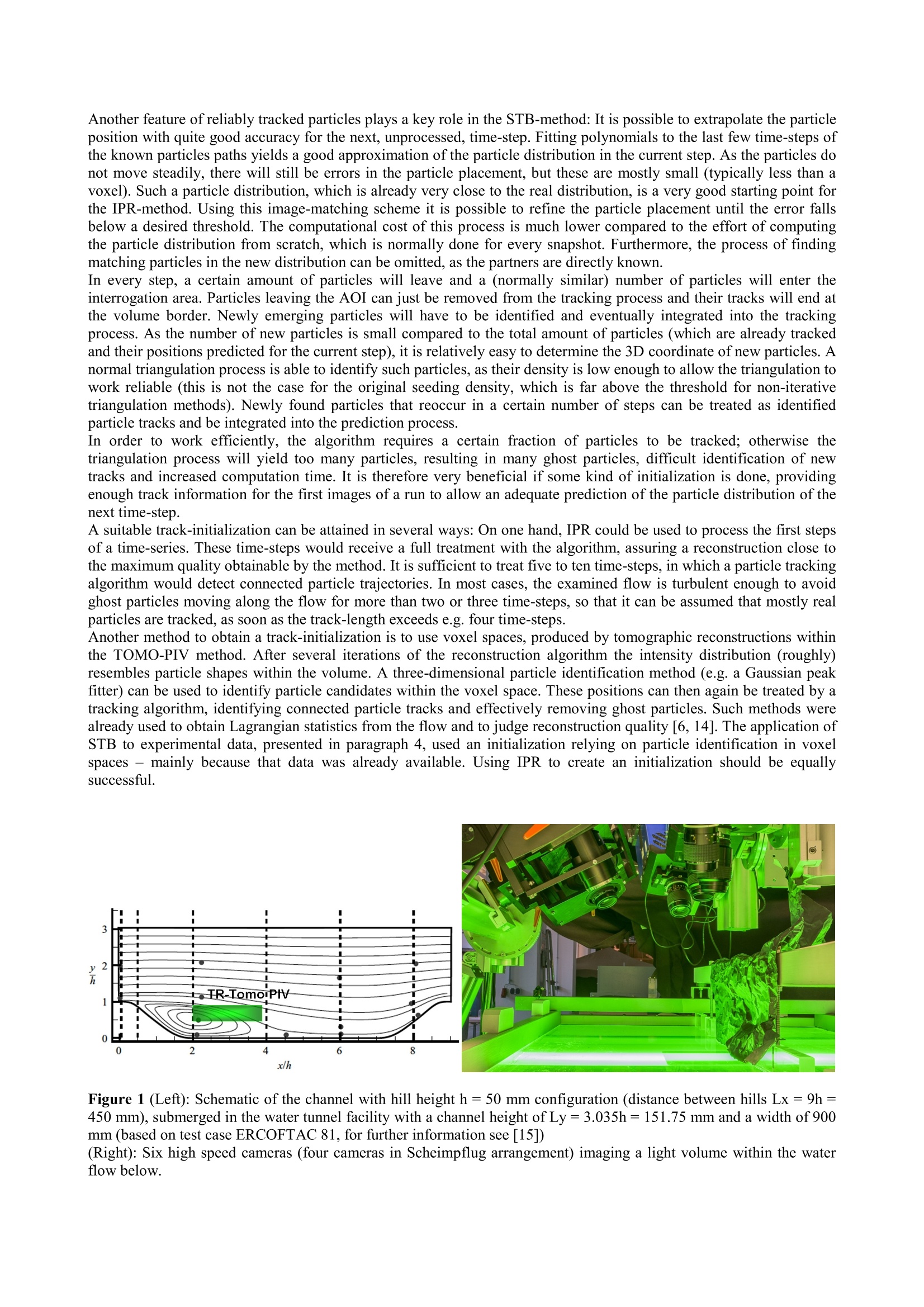
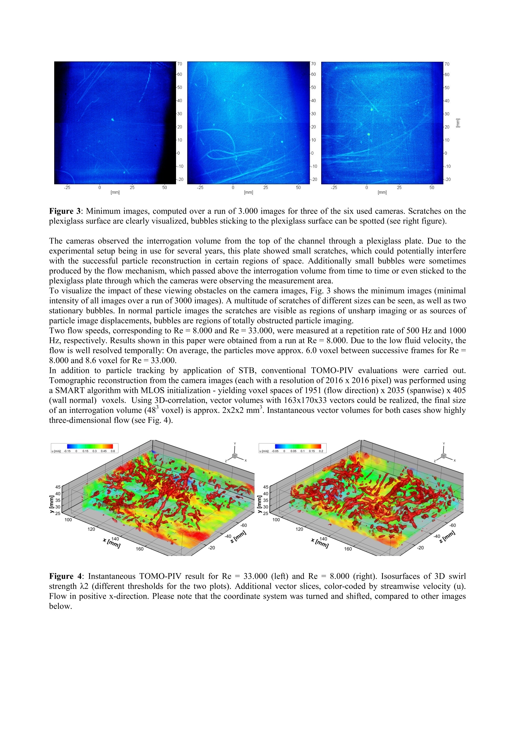
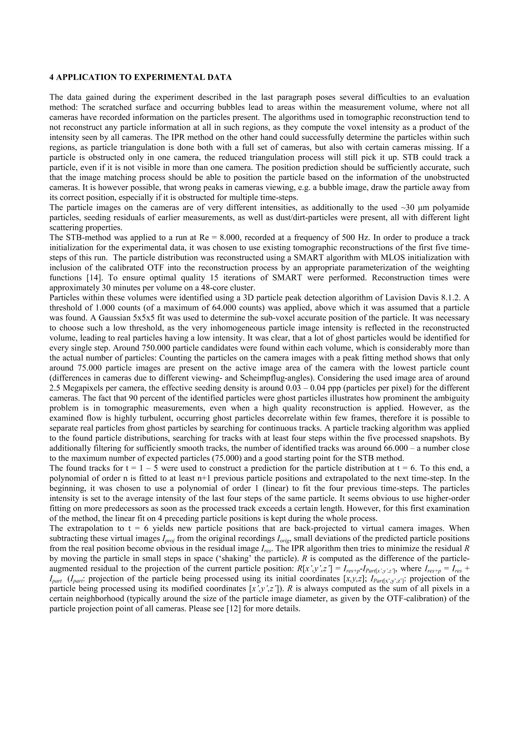
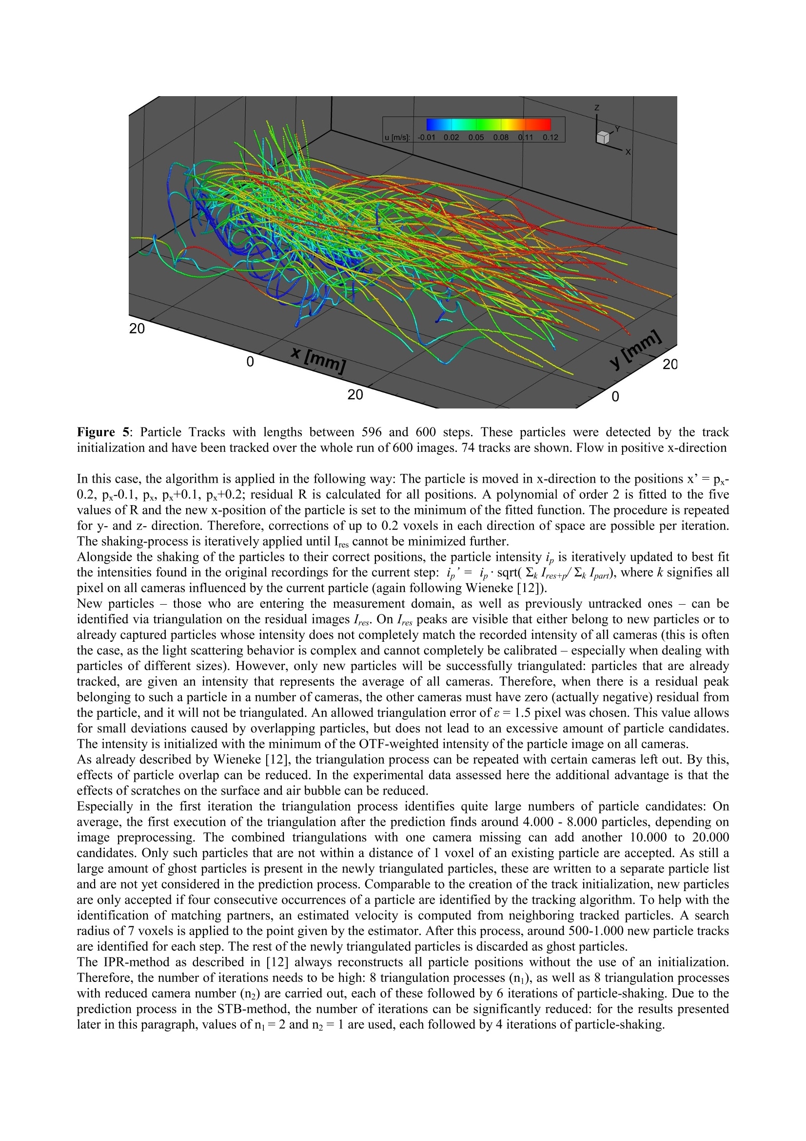
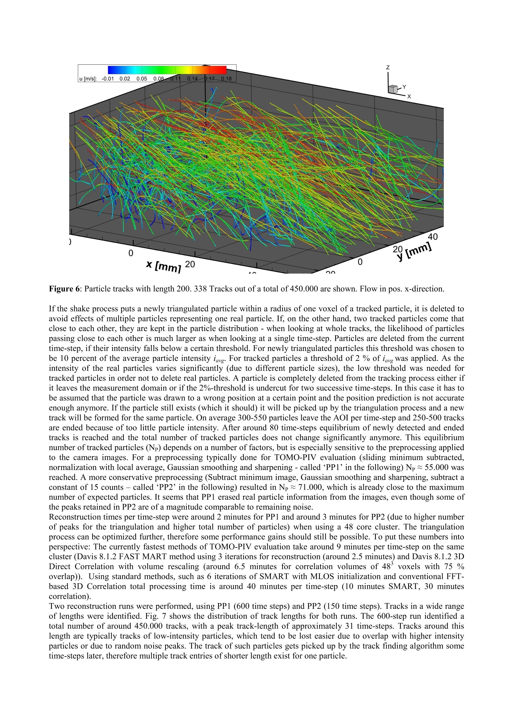
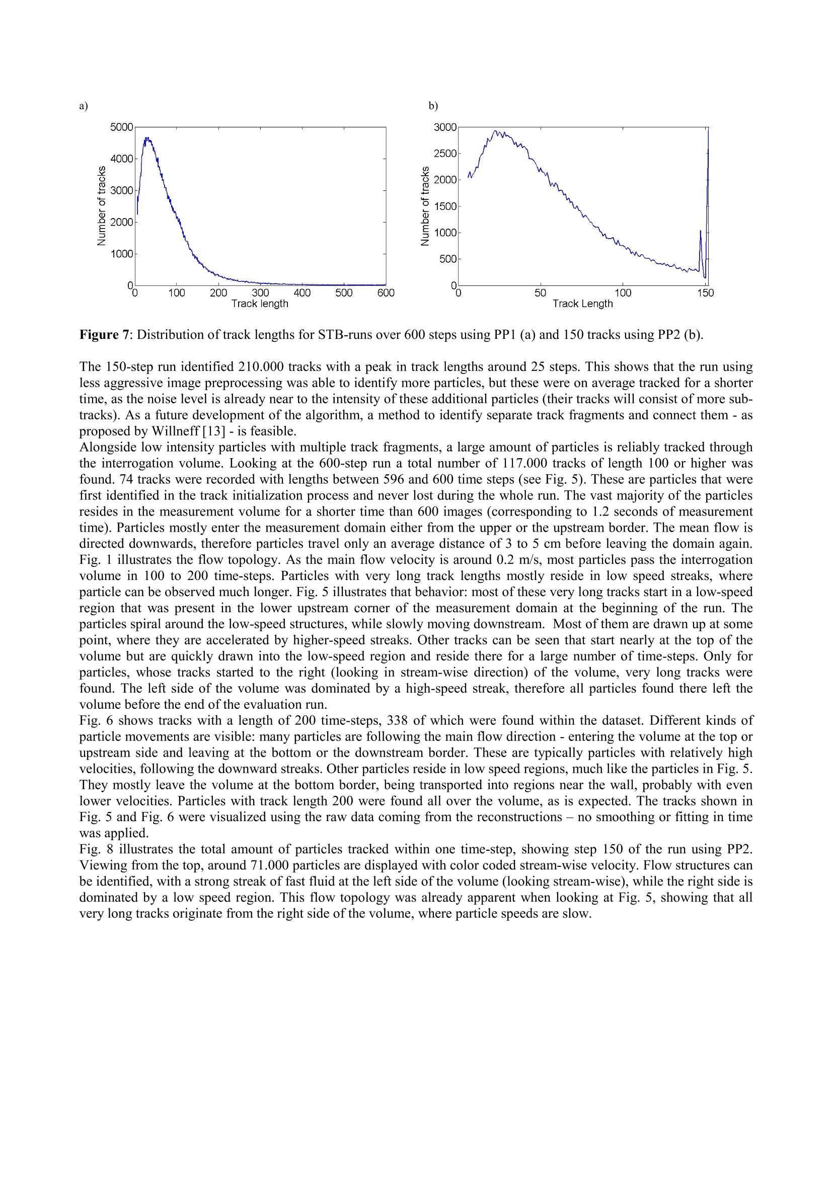
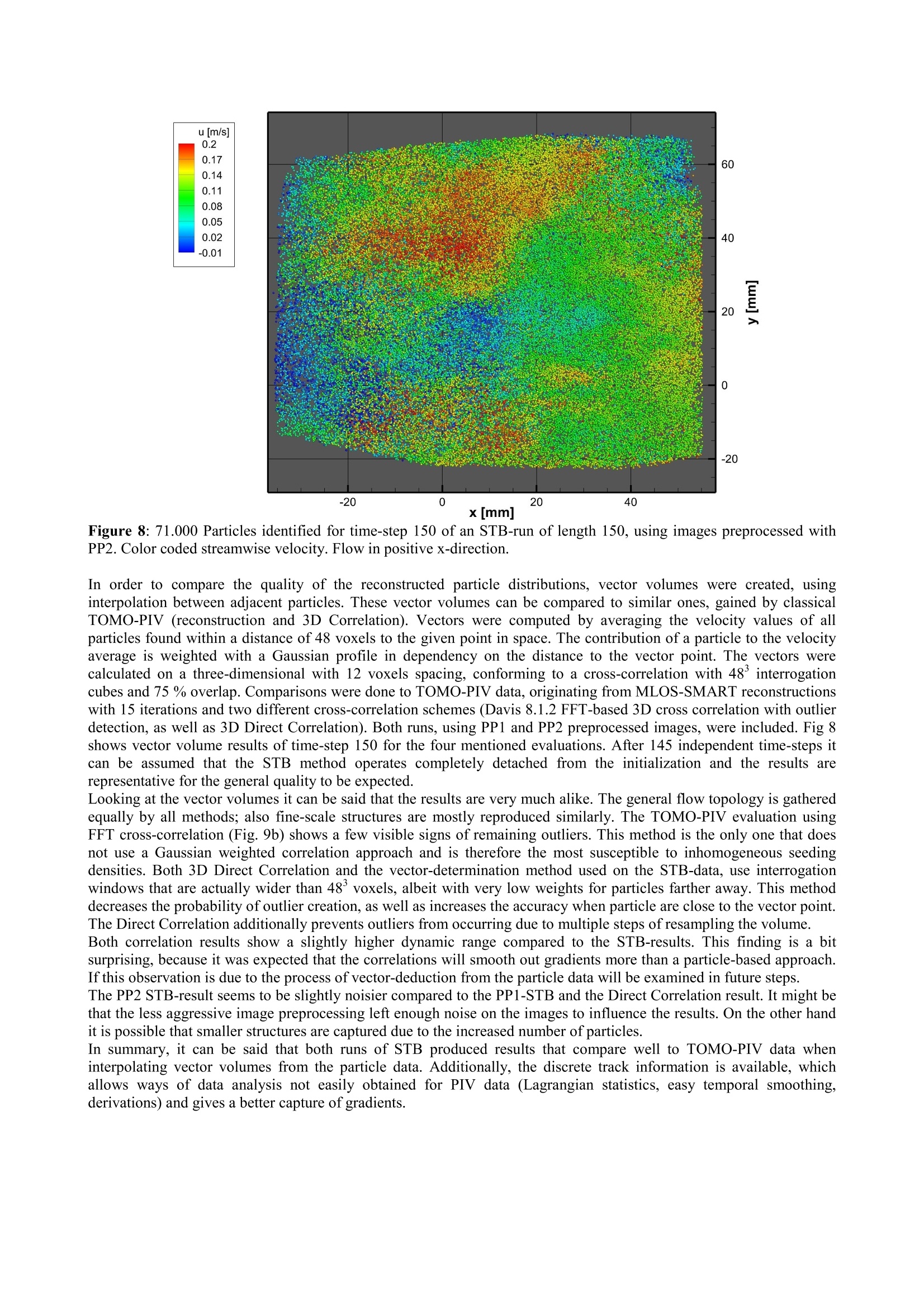
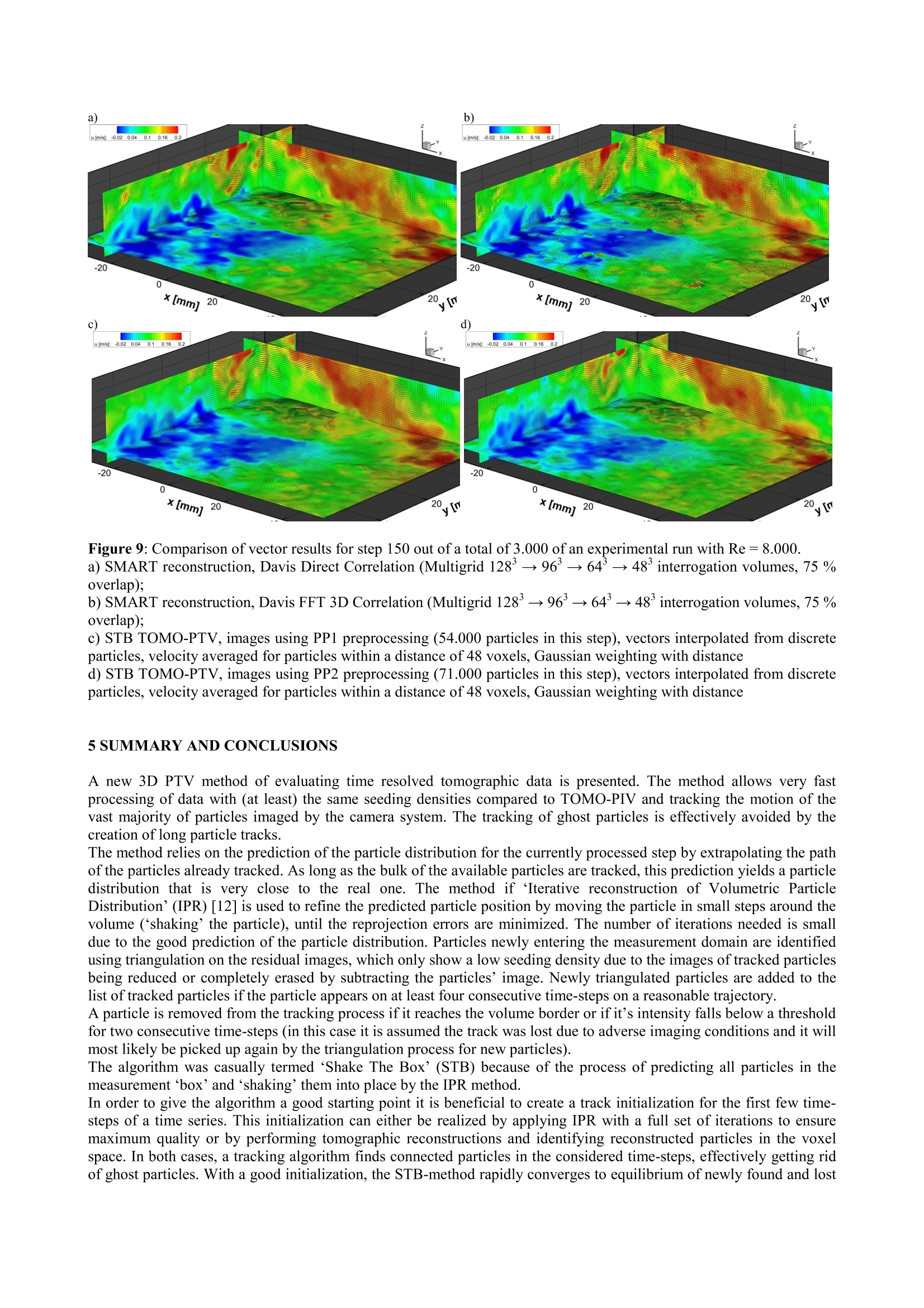
10TH INTERNATIONAL SYMPOSIUM ONPARTICLE IMAGE VELOCIMETRY-PIV13Delft， The Netherlands， July 1-3， 2013 a) ‘Shake The Box'： A highly efficient and accurate Tomographic ParticleTracking Velocimetry (TOMO-PTV) method using prediction of particlepositions Daniel Schanz ， Andreas Schroder'， Sebastian Gesemann'，Dirk Michaelis ，Bernhard Wieneke German Aerospace Center (DLR)， Institute of Aerodynamics and Flow Technology， Germany LaVision GmbH， Gottingen， Germany ABSTRACT A novel approach to the evaluation of time resolved particle-based tomographic data is introduced. By seizing the timeinformation contained in such datasets， a very fast and accurate tracking of nearly all particles within the measurementdomain is achieved at seeding densities comparable to (and probably above) the thresholds for tomographic PIV. Themethod relies on predicting the position of already tracked particles and refining the found position by an imagematching scheme (‘shaking’all particles within the measurement ‘box’until they fit the images： ‘Shake The Box’-STB). New particles entering the measurement domain are identified using triangulation on the residual images. Application of the method on a high-resolution time-resolved experimental dataset showed a reliable tracking of thevast majority of available particles for long time-series with many particles being tracked for their whole length of staywithin the measurement domain. The image matching process ensures highly accurate particle positioning. Comparingthe results to tomographic PIV evaluations by interpolating vector volumes from the discrete particles shows a highconformity of the results. The availability of discrete track information additionally allows for Lagrangian evaluationsnot possible with PIV data， as well as easy temporal smoothing and a reliable determination of derivations. The processing time of a not fully optimized version of STB proved to be a factor of 3 to 4 faster compared to thefastest methods available for TOMO-PIV. 1 INTRODUCTION AND MOTIVATION Since its introduction by Elsinga in 2005， Tomographic PIV (TOMO-PIV) [1， 2] has been rapidly accepted as a reliableand accurate mean of 3D-flow measurements. Applications range from highly resolved measurements in air [3] to time-resolved measurements in water [4] and in air [5， 6]. Like nearly all three-dimensional measurement techniques，TOMO-PIV has to deduct the position in space of the used particle tracers from two-dimensional camera images. Theuse of an iterative approach to this reconstruction， using algorithms like MART or SMART [7， 8] that reconstructparticles as intensity peaks in a voxel space， allows for much higher seeding densities compared to other approaches，such as three-dimensional particle tracking， based on particle triangulation [9]. Using 3d-correlation methods after thereconstructions process ensures a robust deduction of velocity information from the data， reducing negative effects ofghost particle as long as their intensity is below the real particles’intensity. However， some drawbacks are associated with the technique： Ghost particles will always have influence on the vectorresult， especially when using high seeding densities. Furthermore， results gathered from cross-correlation representaverages over interrogation volumes and therefore smooth out velocity gradients and fine flow structures. This effectmight be overcome by the use of adaptive weighting in the correlation process [10] Another downside is the largeamount of computational time needed for the data processing， as well as large amounts of data that need to be (at leasttemporarily) saved to hard disk. When dealing with time-resolved data， it is difficult to use information gained fromother time-steps in the processing of the current one. Methods like ‘Motion Tracking Enhancement’[11] do that， but ata high computational cost. These considerations show that it would be desirable to move from the representation of particles as intensity clusters ina huge voxel-spaceto direct knowledge of particle positions in space. Tracking such particles in time enables precisevelocity determination， without the need of a spatial average. Lagrangian measurements would easily be possible. Thecomputation time could probably be reduced， as the amount of data to be processed is dramatically reduced compared toa voxel space. Three-dimensional Particle Tracking Velocimetry (3D PTV) [9] does exactly that by triangulatingparticles in each time-step and then trying to find matching particles in the different time-steps. However， thetriangulation process is limited by seeding density， allowing only about an order of magnitude fewer particles comparedto TOMO-PIV. The method of Iterative reconstruction of Volumetric Particle Distribution'(IPR)， recently introduced by Wieneke [12]overcomes the problem of limited particle density： in contrast to conventional triangulation methods， an iterativeapproach of particle placement is applied， which allows to process particle numbers that are comparable to typicalTOMO-PIV experiments. The working principle is to compute a distribution of discrete particle positions by iterativelyadding particles， refining their position by moving (shaking’) the particle around in small steps， until an optimum isfound in the particle projection relation to the original images (an image matching approach). Using this method， highlypopulated particle distributions can be reconstructed on a particle basis. Wieneke created voxel spaces from the gainedparticle distribution and showed via 3D-correlation， that the results of IPR are comparable to those of TOMO-PIV. Still，the obtained particle distributions exhibit the problem of ghost particles， possibly interfering with tracking processes.Due to the iterative nature， the processing time of IPR showed to be comparable to a tomographic reconstruction.The method introduced in this paper combines the IPR method with an effective way of seizing the time-information in time-resolved PIV measurements. By this a method is created， which allows a very fast processing of highly seededthree-dimensional data， while capturing the movement of the vast majority of real particles and creating virtually noghost particles. The key step is to produce a prediction ofthe particle distribution in the currently processed step， usingextrapolation of existing particle tracks. This predicted particle distribution is used as an initialization to the IPR processand allows a severe reduction of iterations and therefore processing time. Willneff [13] also used the prediction ofparticle positions in space as a mean of improving particle tracking results， albeit only to close occurring gaps inconventionally created tracks using triangulationn. The general working principle of the method is given in paragraph 2， more detailed explanations are given in paragraph4， where the application to experimental data is illustrated. .2 THE ‘SHAKE THE BOX'METHOD Conventional methods of evaluating highly seeded three-dimensional particle-based measurements rely on an individualtreatment ofevery single snapshot of the particle distribution： Applying TOMO-PIV， a tomographic reconstruction of every time-step is performed， with a subsequent correlation oftwo consecutive voxel spaces. The IPR-method computes the particle distribution from scratch for every snapshot，requiring many iterations until converging to the solution. When dealing with non-time-resolved data， typicallyobtained by low-repetition rate double-frame cameras， such an approach seems reasonable， as only two frames withclosely related solutions to the reconstruction problem are available. As soon though as the data at hand is sufficiently time-resolved， the approaches based on strictly singular imageprocessing neglect the possibility of utilizing already processed data to extract information on the currently processedstep. Therefore， the evaluation of a series from time-resolved experiments proves to be a lengthy process， typicallytaking weeks or months to process on a modern computer cluster. The method presented here seizes the time-information by building predictions of the particle distribution andeffectively refining this initial distribution by image matching， as described by Wieneke [12]. The method was termed‘Shake The Box’(STB) due to the procedure of producing an educated guess of the particles within the ‘box’(measurement domain) and then ‘shaking'the particles around， until an optimal distribution is reached. STB aims to beefficient in terms of calculation time， memory requirements and hard disk space， as well as being highly precise inrespect to the investigated data and producing widely usable data output. Moving from a huge voxel-space to discrete particle positions during the reconstruction phase has several advantages：The amount of main memory needed by the voxel-space can become quite significant； saving the data to hard disk istime consuming and can use vast amounts of space for long time-series. When correlating two voxel spaces both haveto be loaded into the main memory again， requiring read time as well as double the amount of memory. When lookingat the experimental data， presented later in this paper， we see that the used voxel space consists of around2000x2000x400 voxels， equating to 12 GB of data. Saving the reconstructed volumes to disk for later use takes uparound 1 GB per volume (reduction due to data compression) - for the 3000 subsequent images of one run， a totalamount of 3 TB is needed. In comparison， the representation of particles via positions takes up very little space： Typically 6 to 10 values(coordinates， velocities， intensity and other parameters) are associated to a particle per time-step. This means thattypical numbers of particles (50.000 to 100.000， depending on the camera system and volume size) can be stored in lessthan 5 MB of RAM. Writing and reading from hard disk is very fast and the total amount of data for a time-resolved runis normally a few GB. When particle positions are known for single snapshots it is a relatively easy step to find matching partners insuccessive time-steps (as the volume is very sparse compared to the images)- therefore tracking the particles in space ispossible. The knowledge of particle tracks， spanning over multiple time-steps， allows further processing of the data：Fitting the positions in space with suitable functions (polynomials or splines) for a certain amount of time-steps allowsaccounting for noise introduced during the process of particle position identification. Derivations of the velocity (e.g.accelerations) can be computed with better accuracy from such fitted data. Another feature of reliably tracked particles plays a key role in the STB-method： It is possible to extrapolate the particleposition with quite good accuracy for the next， unprocessed， time-step.Fitting polynomials to the last few time-steps ofthe known particles paths yields a good approximation of the particle distribution in the current step. As the particles donot move steadily， there will still be errors in the particle placement， but these are mostly small (typically less than avoxel). Such a particle distribution， which is already very close to the real distribution， is a very good starting point forthe IPR-method. Using this image-matching scheme it is possible to refine the particle placement until the error fallsbelow a desired threshold. The computational cost of this process is much lower compared to the effort of computingthe particle distribution from scratch， which is normally done for every snapshot. Furthermore， the process of findingmatching particles in the new distribution can be omitted， as the partners are directly known. In every step， a certain amount of particles will leave and a (normally similar) number of particles will enter theinterrogation area. Particles leaving the AOI can just be removed from the tracking process and their tracks will end atthe volume border. Newly emerging particles will have to be identified and eventually integrated into the trackingprocess. As the number of new particles is small compared to the total amount of particles (which are already trackedand their positions predicted for the current step)， it is relatively easy to determine the 3D coordinate of new particles. Anormal triangulation process is able to identify such particles， as their density is low enough to allow the triangulation towork reliable (this is not the case for the original seeding density， which is far above the threshold for non-iterativetriangulation methods). Newly found particles that reoccur in a certain number of steps can be treated as identifiedparticle tracks and be integrated into the prediction process. In order to work efficiently， the algorithm requires a certain fraction of particles to be tracked； otherwise thetriangulation process will yield too many particles， resulting in many ghost particles， difficult identification of newtracks and increased computation time. It is therefore very beneficial if some kind of initialization is done， providingenough track information for the first images of a run to allow an adequate prediction of the particle distribution of thenext time-step. A suitable track-initialization can be attained in several ways： On one hand， IPR could be used to process the first stepsof a time-series. These time-steps would receive a full treatment with the algorithm， assuring a reconstruction close tothe maximum quality obtainable by the method. It is sufficient to treat five to ten time-steps， in which a particle trackingalgorithm would detect connected particle trajectories. In most cases， the examined flow is turbulent enough to avoidghost particles moving along the flow for more than two or three time-steps， so that it can be assumed that mostly realparticles are tracked， as soon as the track-length exceeds e.g. four time-steps. Another method to obtain a track-initialization is to use voxel spaces， produced by tomographic reconstructions withinthe TOMO-PIV method. After several iterations of the reconstruction algorithm the intensity distribution (roughly)resembles particle shapes within the volume. A three-dimensional particle identification method (e.g. a Gaussian peakfitter) can be used to identify particle candidates within the voxel space. These positions can then again be treated by atracking algorithm， identifying connected particle tracks and effectively removing ghost particles. Such methods werealready used to obtain Lagrangian statistics from the flow and to judge reconstruction quality [6， 14]. The application ofSTB to experimental data， presented in paragraph 4， used an initialization relying on particle identification in voxelspaces - mainly because that data was already available. Using IPR to create an initialization should be equallysuccessful. Figure 1 (Left)： Schematic of the channel with hill height h= 50 mm configuration (distance between hills Lx=9h =450 mm)， submerged in the water tunnel facility with a channel height of Ly=3.035h=151.75 mm and a width of 900mm (based on test case ERCOFTAC 81， for further information see [15]) (Right)： Six high speed cameras (four cameras in Scheimpflug arrangement) imaging a light volume within the waterflow below. Using the particle tracks for time-steps 1-n gained from the initialization it is possible to predict the particle distributionfor time n+1 and from there on iterate the depicted algorithm， extending the known particle track from step to step，optimizing the new positions by shaking (image matching) and successively adding newly found particle tracks. TheSTB-method works its way through a time-series， always creating the information needed to effectively process the nexttime-step by refining the result of the currently processed step. A more detailed description of the methods’application to an experimental dataset - introduced below -is presented inparagraph 4. 3 EXPERIMENTAL SETUP An experiment， conducted within the scope of the EU-FP7 project AFDAR (Advanced Flow Diagnostics for Aeronautical Research')， will be used to demonstrate the applicability of the STB-method to real experimental data.The experiment took place in the water tunnel facility at Technical University of Munich. The flow behind a series ofidentical longitudinal hills (‘periodic hills’， ERCOFTAC test-case 81[15]) was investigated using a high-speedtomographic PIV system. Six Imager pro HS 4M (PCO Dimax) cameras were used to observe a measurement volumeof 80x80x20 mm， located 2 h(100 mm) downstream of the seventh hill (the experiment uses of a total of tenconsecutive hills). Wall-normal height spans from 25 to 45 mm in order to capture the shear layer (see Fig. 1). Thewater was seeded using ~30 um polyamide particles. Illumination was realized using a Quantronix Darwin Duocontinuous laser， provided by UNIBWM. The laser beam was widened by two successive telescope optics usingcylindrical lenses， resulting in an oval light profile. The profile was cut in rectangular shape by a passe-partout that wasfixed at the side wall of the channel. This volume light sheet passes through the interrogation volume and is back-reflected into itself using an end-mirror located directly outside of the opposite wall of the tunnel [5]. A second passe-partout is installed there. This setup enables all cameras to be in forward scattering and thus gather a maximum of light.In order to assure sufficient contrast for the imaged particles， a sheet of black adhesive foil was installed below theilluminated area. Due to space restrictions four cameras were placed in line， whereas two of them observed the measurement volume inan off-axis arrangement. The four outermost cameras had to be equipped with Scheimpflug-adapters due to theirviewing angle relative to the measurement volume. Five cameras used 105 mm Nikon Micro Nikkor lenses， while onecamera used a 100 mm Zeiss Distagon Macro lens. The strong scattering of light by the particles allowed closing theapertures to F#= 22， minimizing particle blurring effects due to limited depth of field or astigmatisms. An averageresolution of approx. 21.5 pixels per mm was achieved. Calibration was done using a 3D-calibration-plate， providing two planes of calibration markers， thus requiring no wall-normal movement of the plate. A carrier was constructed， securing the plate firmly between the two neighbouring hills(see Fig. 2). The carrier was fixed in spanwise direction using strong magnets at the side walls of the tunnel. Small，inevitable errors of the calibration were corrected by applying the method of volume-self-calibration (VSC) [16] to theparticle images. Back-projection errors of around 1 pixel were found and corrected to values below 0.02 pixels by thismethod. Alongside the VSC， a calibration of the optical transfer function (OTF) [14] was performed， gathering theaveraged particle imaging form different areas of the measurement domain on the camera images. As indicated byWieneke， the use of a calibrated OTF is very beneficial to the accuracy of particle placement using IPR. Figure 2： Two-plane calibration target positioned in the middle of the test section on a carrier with negative hills anddistance holders to the side-walls. Upper plane located at y=35 mm. Figure 3： Minimum images， computed over a run of 3.000 images for three of the six used cameras. Scratches on theplexiglass surface are clearly visualized， bubbles sticking to the plexiglass surface can be spotted (see right figure). The cameras observed the interrogation volume from the top of the channel through a plexiglass plate. Due to theexperimental setup being in use for several years， this plate showed small scratches， which could potentially interferewith the successful particle reconstruction in certain regions of space. Additionally small bubbles were sometimesproduced by the flow mechanism， which passed above the interrogation volume from time to time or even sticked to theplexiglass plate through which the cameras were observing the measurement area. To visualize the impact of these viewing obstacles on the camera images， Fig. 3 shows the minimum images (minimalintensity of all images over a run of 3000 images). A multitude of scratches of different sizes can be seen， as well as twostationary bubbles. In normal particle images the scratches are visible as regions of unsharp imaging or as sources ofparticle image displacements， bubbles are regions of totally obstructed particle imaging. Two flow speeds， corresponding to Re =8.000 and Re=33.000， were measured at a repetition rate of 500 Hz and 1000Hz， respectively. Results shown in this paper were obtained from a run at Re=8.000. Due to the low fluid velocity， theflow is well resolved temporally： On average， the particles move approx. 6.0 voxel between successive frames for Re=8.000 and 8.6 voxel for Re =33.000. In addition to particle tracking by application of STB， conventional TOMO-PIV evaluations were carried out.Tomographic reconstruction from the camera images (each with a resolution of 2016 x 2016 pixel) was performed usinga SMART algorithm with MLOS initialization - yielding voxel spaces of 1951 (flow direction) x 2035 (spanwise) x 405(wall normal) voxels. Using 3D-correlation， vector volumes with 163x170x33 vectors could be realized， the final sizeof an interrogation volume (48’voxel) is approx.2x2x2 mm’. Instantaneous vector volumes for both cases show highlythree-dimensional flow (see Fig.4). Figure 4： Instantaneous TOMO-PIV result for Re =33.000 (left) and Re =8.000 (right). Isosurfaces of 3D swirlstrength A2 (different thresholds for the two plots). Additional vector slices， color-coded by streamwise velocity (u).Flow in positive x-direction. Please note that the coordinate system was turned and shifted， compared to other imagesbelow. 4 APPLICATION TO EXPERIMENTAL DATA The data gained during the experiment described in the last paragraph poses several difficulties to an evaluationmethod： The scratched surface and occurring bubbles lead to areas within the measurement volume， where not allcameras have recorded information on the particles present. The algorithms used in tomographic reconstruction tend tonot reconstruct any particle information at all in such regions， as they compute the voxel intensity as a product of theintensity seen by all cameras. The IPR method on the other hand could successfully determine the particles within suchregions， as particle triangulation is done both with a full set of cameras， but also with certain cameras missing. If aparticle is obstructed only in one camera， the reduced triangulation process will still pick it up. STB could track aparticle， even if it is not visible in more than one camera. The position prediction should be sufficiently accurate， suchthat the image matching process should be able to position the particle based on the information of the unobstructedcameras. It is however possible， that wrong peaks in cameras viewing， e.g. a bubble image，draw the particle away fromits correct position， especially if it is obstructed for multiple time-steps. The particle images on the cameras are of very different intensities， as additionally to the used ~30 um polyamideparticles， seeding residuals of earlier measurements， as well as dust/dirt-particles were present， all with different lightscattering properties. The STB-method was applied to a run at Re =8.000， recorded at a frequency of 500 Hz. In order to produce a trackinitialization for the experimental data， it was chosen to use existing tomographic reconstructions of the first five time-steps of this run. The particle distribution was reconstructed using a SMART algorithm with MLOS initialization withinclusion of the calibrated OTF into the reconstruction process by an appropriate parameterization of the weightingfunctions [14]. To ensure optimal quality 15 iterations of SMART were performed. Reconstruction times wereapproximately 30 minutes per volume on a 48-core cluster. Particles within these volumes were identified using a 3D particle peak detection algorithm of Lavision Davis 8.1.2. Athreshold of 1.000 counts (of a maximum of 64.000 counts) was applied， above which it was assumed that a particlewas found. A Gaussian 5x5x5 fit was used to determine the sub-voxel accurate position of the particle. It was necessaryto choose such a low threshold， as the very inhomogeneous particle image intensity is reflected in the reconstructedvolume， leading to real particles having a low intensity. It was clear， that a lot of ghost particles would be identified forevery single step. Around 750.000 particle candidates were found within each volume， which is considerably more thanthe actual number of particles： Counting the particles on the camera images with a peak fitting method shows that onlyaround 75.000 particle images are present on the active image area of the camera with the lowest particle count(differences in cameras due to different viewing- and Scheimpflug-angles). Considering the used image area of around2.5 Megapixels per camera， the effective seeding density is around 0.03 -0.04 ppp (particles per pixel) for the differentcameras. The fact that 90 percent of the identified particles were ghost particles illustrates how prominent the ambiguityproblem is in tomographic measurements， even when a high quality reconstruction is applied. However， as theexamined flow is highly turbulent， occurring ghost particles decorrelate within few frames， therefore it is possible toseparate real particles from ghost particles by searching for continuous tracks. A particle tracking algorithm was appliedto the found particle distributions， searching for tracks with at least four steps within the five processed snapshots. Byadditionally filtering for sufficiently smooth tracks， the number of identified tracks was around 66.000 - a number closeto the maximum number of expected particles (75.000) and a good starting point for the STB method. The found tracks for t =1- 5 were used to construct a prediction for the particle distribution at t=6. To this end， apolynomial of order n is fitted to at least n+1 previous particle positions and extrapolated to the next time-step. In thebeginning， it was chosen to use a polynomial of order 1 (linear) to fit the four previous time-steps. The particlesintensity is set to the average intensity of the last four steps of the same particle. It seems obvious to use higher-orderfitting on more predecessors as soon as the processed track exceeds a certain length. However， for this first examinationof the method， the linear fit on 4 preceding particle positions is kept during the whole process. The extrapolation to t= 6 yields new particle positions that are back-projected to virtual camera images. Whensubtracting these virtual images Iproj from the original recordings Iorig， small deviations of the predicted particle positionsfrom the real position become obvious in the residual image Ires. The IPR algorithm then tries to minimize the residual Rby moving the particle in small steps in space (shaking’the particle). R is computed as the difference of the particle-augmented residual to the projection of the current particle position： R[x'，y'z]=Ires+p-IPart x’，yz]， where Ires+p =Ires +Ipart (Ipart： projection of the particle being processed using its initial coordinates [x，y，z]； IPart[x’，y，z]： projection of theparticle being processed using its modified coordinates [x’，y，z]). R is always computed as the sum of all pixels in acertain neighborhood (typically around the size of the particle image diameter， as given by the OTF-calibration) of theparticle projection point of all cameras. Please see [12] for more details. Figure 5： Particle Tracks with lengths between 596 and 600 steps. These particles were detected by the trackinitialization and have been tracked over the whole run of 600 images. 74 tracks are shown. Flow in positive x-direction In this case， the algorithm is applied in the following way： The particle is moved in x-direction to the positions x’=px-0.2， px-0.1， px， px+0.1， px+0.2； residual R is calculated for all positions. A polynomial of order 2 is fitted to the fivevalues of R and the new x-position of the particle is set to the minimum of the fitted function. The procedure is repeatedfor y- and z- direction. Therefore， corrections of up to 0.2 voxels in each direction of space are possible per iteration.The shaking-process is iteratively applied until Ires cannot be minimized further. Alongside the shaking of the particles to their correct positions， the particle intensity i， is iteratively updated to best fitthe intensities found in the original recordings for the current step： ip'=ipsqrt( Ires+p2k Ipart)， where k signifies allpixel on all cameras influenced by the current particle (again following Wieneke [12]). New particles -those who are entering the measurement domain， as well as previously untracked ones - can beidentified via triangulation on the residual images Ires. On Ires peaks are visible that either belong to new particles or toalready captured particles whose intensity does not completely match the recorded intensity of all cameras (this is oftenthe case， as the light scattering behavior is complex and cannot completely be calibrated - especially when dealing withparticles of different sizes). However， only new particles will be successfully triangulated： particles that are alreadytracked， are given an intensity that represents the average of all cameras. Therefore， when there is a residual peakbelonging to such a particle in a number of cameras， the other cameras must have zero (actually negative) residual fromthe particle， and it will not be triangulated. An allowed triangulation error of e=1.5 pixel was chosen. This value allowsfor small deviations caused by overlapping particles， but does not lead to an excessive amount of particle candidates.The intensity is initialized with the minimum of the OTF-weighted intensity of the particle image on all cameras. As already described by Wieneke [12]， the triangulation process can be repeated with certain cameras left out. By this，effects of particle overlap can be reduced. In the experimental data assessed here the additional advantage is that theeffects of scratches on the surface and air bubble can be reduced. Especially in the first iteration the triangulation process identifies quite large numbers of particle candidates： Onaverage， the first execution of the triangulation after the prediction finds around 4.000-8.000 particles， depending onimage preprocessing. The combined triangulations with one camera missing can add another 10.000 to 20.000candidates. Only such particles that are not within a distance of 1 voxel of an existing particle are accepted. As still alarge amount of ghost particles is present in the newly triangulated particles， these are written to a separate particle listand are not yet considered in the prediction process. Comparable to the creation of the track initialization， new particlesare only accepted if four consecutive occurrences of a particle are identified by the tracking algorithm. To help with theidentification of matching partners， an estimated velocity is computed from neighboring tracked particles. A searchradius of 7 voxels is applied to the point given by the estimator. After this process， around 500-1.000 new particle tracksare identified for each step. The rest of the newly triangulated particles is discarded as ghost particles. The IPR-method as described in [12] always reconstructs all particle positions without the use of an initialization.Therefore， the number of iterations needs to be high： 8 triangulation processes (ni)， as well as 8 triangulation processeswith reduced camera number (n2) are carried out， each of these followed by 6 iterations of particle-shaking. Due to theprediction process in the STB-method， the number of iterations can be significantly reduced： for the results presentedlater in this paragraph， values of n=2 and n2=1 are used， each followed by 4 iterations of particle-shaking. Figure 6： Particle tracks with length 200.338 Tracks out of a total of 450.000 are shown. Flow in pos. x-direction. If the shake process puts a newly triangulated particle within a radius of one voxel of a tracked particle， it is deleted toavoid effects of multiple particles representing one real particle. If， on the other hand， two tracked particles come thatclose to each other， they are kept in the particle distribution - when looking at whole tracks， the likelihood of particlespassing close to each other is much larger as when looking at a single time-step. Particles are deleted from the currenttime-step， if their intensity falls below a certain threshold. For newly triangulated particles this threshold was chosen tobe 10 percent of the average particle intensity iavg. For tracked particles a threshold of 2 % of iavg was applied. As theintensity of the real particles varies significantly (due to different particle sizes)， the low threshold was needed fortracked particles in order not to delete real particles. A particle is completely deleted from the tracking process either ifit leaves the measurement domain or if the 2%-threshold is undercut for two successive time-steps. In this case it has tobe assumed that the particle was drawn to a wrong position at a certain point and the position prediction is not accurateenough anymore. If the particle still exists (which it should) it will be picked up by the triangulation process and a newtrack will be formed for the same particle.On average 300-550 particles leave the AOI per time-step and 250-500 tracksare ended because of too little particle intensity. After around 80 time-steps equilibrium of newly detected and endedtracks is reached and the total number of tracked particles does not change significantly anymore. This equilibriumnumber of tracked particles (Np) depends on a number of factors， but is especially sensitive to the preprocessing appliedto the camera images. For a preprocessing typically done for TOMO-PIV evaluation (sliding minimum subtracted，nor zation withh 1 local average， Gaussian smoothing and sharpening-called ‘PP1’in the following) Np~55.000 wasreached. A more conservative preprocessing (Subtract minimum image， Gaussian smoothing and sharpening， subtract aconstant of 15 counts - called ‘PP2’in the following) resulted in Np ~ 71.000， which is already close to the maximumnumber of expected particles. It seems that PP1 erased real particle information from the images， even though some ofthe peaks retained in PP2 are of a magnitude comparable to remaining noise. Reconstruction times per time-step were around 2 minutes for PP1 and around 3 minutes for PP2 (due to higher numberof peaks for the triangulation and higher total number of particles) when using a 48 core cluster. The triangulationprocess can be optimized further， therefore some performance gains should still be possible. To put these numbers intoperspective： The currently fastest methods of TOMO-PIV evaluation take around 9 minutes per time-step on the samecluster (Davis 8.1.2 FAST MART method using 3 iterations for reconstruction (around 2.5 minutes) and Davis 8.1.2 3DDirect Correlation with volume rescaling (around 6.5 minutes for correlation volumes of 48’ voxels with 75 %overlap)). Using standard methods， such as 6 iterations of SMART with MLOS initialization and conventional FFT-based 3D Correlation total processing time is around 40 minutes per time-step (10 minutes SMART， 30 minutescorrelation). Two reconstruction runs were performed， using PP1 (600 time steps) and PP2 (150 time steps). Tracks in a wide rangeof lengths were identified. Fig. 7 shows the distribution of track lengths for both runs. The 600-step run identified atotal number ofaround 450.000 tracks， with a peak track-length of approximately 31 time-steps. Tracks around thislength are typically tracks of low-intensity particles， which tend to be lost easier due to overlap with higher intensityparticles or due to random noise peaks. The track of such particles gets picked up by the track finding algorithm sometime-steps later， therefore multiple track entries of shorter length exist for one particle. Figure 7： Distribution of track lengths for STB-runs over 600 steps using PP1 (a) and 150 tracks using PP2 (b). The 150-step run identified 210.000 tracks with a peak in track lengths around 25 steps. This shows that the run usingless aggressive image preprocessing was able to identify more particles， but these were on average tracked for a shortertime， as the noise level is already near to the intensity of these additional particles (their tracks will consist of more sub-tracks). As a future development of the algorithm， a method to identify separate track fragments and connect them -asproposed by Willneff [13]-is feasible. Alongside low intensity particles with multiple track fragments， a large amount of particles is reliably tracked throughthe interrogation volume. Looking at the 600-step run a total number of 117.000 tracks of length 100 or higher wasfound. 74 tracks were recorded with lengths between 596 and 600 time steps (see Fig. 5). These are particles that werefirst identified in the track initialization process and never lost during the whole run. The vast majority of the particlesresides in the measurement volume for a shorter time than 600 images (corresponding to 1.2 seconds of measurementtime). Particles mostly enter the measurement domain either from the upper or the upstream border. The mean flow isdirected downwards， therefore particles travel only an average distance of 3 to 5 cm before leaving the domain again.Fig. 1 illustrates the flow topology. As the main flow velocity is around 0.2 m/s， most particles pass the interrogationvolume in 100 to 200 time-steps. Particles with very long track lengths mostly reside in low speed streaks， whereparticle can be observed much longer. Fig. 5 illustrates that behavior： most of these very long tracks start in a low-speedregion that was present in the lower upstream corner of the measurement domain at the beginning of the run. Theparticles spiral around the low-speed structures， while slowly moving downstream. Most of them are drawn up at somepoint， where they are accelerated by higher-speed streaks. Other tracks can be seen that start nearly at the top of thevolume but are quickly drawn into the low-speed region and reside there for a large number of time-steps. Only forparticles， whose tracks started to the right (looking in stream-wise direction) of the volume， very long tracks werefound. The left side of the volume was dominated by a high-speed streak， therefore all particles found there left thevolume before the end of the evaluation run. Fig.6 shows tracks with a length of 200 time-steps， 338 of which were found within the dataset. Different kinds ofparticle movements are visible： many particles are following the main flow direction- entering the volume at the top orupstream side and leaving at the bottom or the downstream border. These are typically particles with relatively highvelocities， following the downward streaks. Other particles reside in low speed regions， much like the particles in Fig. 5.They mostly leave the volume at the bottom border， being transported into regions near the wall， probably with evenlower velocities. Particles with track length 200 were found all over the volume， as is expected. The tracks shown inFig. 5 and Fig. 6 were visualized using the raw data coming from the reconstructions - no smoothing or fitting in timewas applied. Fig. 8 illustrates the total amount of particles tracked within one time-step， showing step 150 of the run using PP2.Viewing from the top， around 71.000 particles are displayed with color coded stream-wise velocity. Flow structures canbe identified， with a strong streak of fast fluid at the left side of the volume (looking stream-wise)， while the right side isdominated by a low speed region. This flow topology was already apparent when looking at Fig. 5， showing that allvery long tracks originate from the right side of the volume， where particle speeds are slow. E二> x[mm] Figure 8： 71.000 Particles identified for time-step 150 of an STB-run of length 150， using images preprocessed withPP2. Color coded streamwise velocity. Flow in positive x-direction. In order to compare the quality of the reconstructed particle distributions， vector volumes were created， usinginterpolation between adjacent particles. These vector volumes can be compared to similar ones， gained by classicalTOMO-PIV (reconstruction and 3D Correlation). Vectors were computed by averaging the velocity values of allparticles found within a distance of 48 voxels to the given point in space. The contribution of a particle to the velocityaverage is weighted with a Gaussian profile in dependency on the distance to the vector point. The vectors werecalculated on a three-dimensional with 12 voxels spacing， conforming to a cross-correlation with 48interrogationcubes and 75 % overlap. Comparisons were done to TOMO-PIV data， originating from MLOS-SMART reconstructionswith 15 iterations and two different cross-correlation schemes (Davis 8.1.2 FFT-based 3D cross correlation with outlierdetection， as well as 3D Direct Correlation). Both runs， using PP1 and PP2 preprocessed images， were included. Fig 8shows vector volume results of time-step 150 for the four mentioned evaluations. After 145 independent time-steps itcan be assumed that the STB method operates completely detached from the initialization and the results arerepresentative for the general quality to be expected. Looking at the vector volumes it can be said that the results are very much alike. The general flow topology is gatheredequally by all methods； also fine-scale structures are mostly reproduced similarly. The TOMO-PIV evaluation usingFFT cross-correlation (Fig. 9b) shows a few visible signs of remaining outliers. This method is the only one that doesnot use a Gaussian weighted correlation approach and is therefore the most susceptible to inhomogeneous seedingdensities. Both 3D Direct Correlation and the vector-determination method used on the STB-data， use interrogationwindows that are actually wider than 48’voxels， albeit with very low weights for particles farther away. This methoddecreases the probability of outlier creation， as well as increases the accuracy when particle are close to the vector point.The Direct Correlation additionally prevents outliers from occurring due to multiple steps of resampling the volume. Both correlation results show a slightly higher dynamic range compared to the STB-results. This finding is a bitsurprising， because it was expected that the correlations will smooth out gradients more than a particle-based approach.If this observation is due to the process of vector-deduction from the particle data will be examined in future steps. The PP2 STB-result seems to be slightly noisier compared to the PP1-STB and the Direct Correlation result. It might bethat the less aggressive image preprocessing left enough noise on the images to influence the results. On the other handit is possible that smaller structures are captured due to the increased number of particles. In summary， it can be said that both runs of STB produced results that compare well to TOMO-PIV data wheninterpolating vector volumes from the particle data. Additionally， the discrete track information is available， whichallows ways of data analysis not easily obtained for PIV data (Lagrangian statistics， easy temporal smoothing，derivations) and gives a better capture of gradients. a) b) c) d) um/s]： -0.02 0.04 0.1 0.160.2 trY -20 0 x[mm]20 20 Figure 9： Comparison of vector results for step 150 out of a total of 3.000 of an experimental run with Re=8.000. a) SMART reconstruction， Davis Direct Correlation (Multigrid 128-96→64-48interrogation volumes， 75%overlap)； b) SMART reconstruction， Davis FFT 3D Correlation (Multigrid 128’-96-64-48'interrogation volumes， 75%overlap)； c) STB TOMO-PTV，images using PP1 preprocessing (54.000 particles in this step)， vectors interpolated from discreteparticles， velocity averaged for particles within a distance of 48 voxels， Gaussian weighting with distance d) STB TOMO-PTV， images using PP2 preprocessing (71.000 particles in this step)， vectors interpolated from discreteparticles， velocity averaged for particles within a distance of 48 voxels， Gaussian weighting with distance 5 SUMMARY AND CONCLUSIONS A new 3D PTV method of evaluating time resolved tomographic data is presented. The method allows very fastprocessing of data with (at least) the same seeding densities compared to TOMO-PIV and tracking the motion of thevast majority of particles imaged by the camera system. The tracking of ghost particles is effectively avoided by thecreation of long particle tracks. The method relies on the prediction of the particle distribution for the currently processed step by extrapolating the pathof the particles already tracked. As long as the bulk of the available particles are tracked， this prediction yields a particledistribution that is very close to the real one. The method if ‘Iterative reconstruction of Volumetric ParticleDistribution’(IPR) [12] is used to refine the predicted particle position by moving the particle in small steps around thevolume (shaking’the particle)， until the reprojection errors are minimized. The number of iterations needed is smalldue to the good prediction of the particle distribution. Particles newly entering the measurement domain are identifiedusing triangulation on the residual images， which only show a low seeding density due to the images of tracked particlesbeing reduced or completely erased by subtracting the particles’ image. Newly triangulated particles are added to thelist of tracked particles if the particle appears on at least four consecutive time-steps on a reasonable trajectory.A particle is removed from the tracking process if it reaches the volume border or if it’s intensity falls below a threshold for two consecutive time-steps (in this case it is assumed the track was lost due to adverse imaging conditions and it willmost likely be picked up again by the triangulation process for new particles). The algorithm was casually termed ‘Shake The Box’(STB) because of the process of predicting all particles in themeasurement ‘box’and‘shaking’them into place by the IPR method. In order to give the algorithm a good starting point it is beneficial to create a track initialization for the first few time-steps of a time series. This initialization can either be realized by applying IPR with a full set of iterations to ensuremaximum quality or by performing tomographic reconstructions and identifying reconstructed particles in the voxelspace. In both cases， a tracking algorithm finds connected particles in the considered time-steps， effectively getting ridof ghost particles. With a good initialization， the STB-method rapidly converges to equilibrium of newly found and lost particles. The number of identified particles is close to the total number of particles within the measurement domain， ifimage preprocessing is applied that does not eradicate images of real particles. Due to the reliable prediction of particle positions， the method performs very fast. The processing time of the used (notcompletely optimized) version of STB was a factor of 3 to 4 shorter compared to the currently fastest TOMO-PIVevaluation methods. When comparing to standard methods， the factor is around 14 to20. The STB-method was applied to an experimental dataset on the flow behind a series of periodic hills at Re=8.000，recorded at a frequency of 500 Hz. On average， the particles move around 6 voxels between frames. A trackinitialization was created using existing tomographic reconstructions of the first five images. Two runs of STB wereperformed using different preprocessing settings for the camera images (length： 150 and 600 frames). It was shown thatboth runs converge to a stable number of tracked particles (55.000 for a rather strong preprocessing， 71.000 for a moreconservative one). The maximum number of expected particles is around 75.000 (as shown by a peak finder applied tothe camera images). Particle intensities of the investigated data vary significantly， thus a stronger preprocessing leads toa loss of real particles. The remaining particles are tracked reliable， however. The occurrence of multiple particle tracksfor one particle is decreased， compared to the run using mild preprocessing. Many particles are correctly tracked fortheir whole length of stay in the measurement domain. The 600-step run showed 117.000 tracks with length above 100steps， some particles were tracked for all 600 images. A comparison to TOMO-PIV evaluations was done by creating vector volumes from the discrete particle distributions.These were compared to similar volumes calculated by state-of-the-art TOMO-PIV evaluation algorithms. Only veryminor differences were found， showing that the quality of the data gathered by the STB-method is comparable toTOMO-PIV， even when giving up the greatest advantage - the knowledge of real particle trajectories - for spaceaveraged vector representation. The whole process of applying STB to experimental data showed a very reliable and stable behavior of the method. Theresults were less depending on the different parameters of the algorithm than on the input (namely the preprocessingused on the images). Considering the problematic quality of the images (scratches on the plexiglass interface， bubbleson the surface， varying particle intensities) this is a good sign for the easy applicability of the method on variousdatasets， as long as the time-resolution is sufficient. 6 OUTLOOK The features of the STB-method that until now were captured only qualitatively using experimental data will bequantified using a synthetic dataset with known ground truth. STB exhibits some more advantages over other evaluationschemes not seizing the time information， which will be investigated in the future. The method should be able to dealwith images with higher seeding densities， compared to TOMO-PIV or single-frame IPR. The knowledge of particletracks enables an efficient reduction of the parameter space and reduces the ‘effective’seeding density. Using syntheticdata it will be assessed how STB compares to TOMO-PIV and IPR at high seeding densities. As indicated by Wieneke[12]， the accuracy of particle placement using IPR (image matching) should be better compared to TOMO-PIV-at leastup to seeding densities of 0.1 ppp. It will be assessed if this still holds true for the STB-method and if furtherimprovements can be made when using high seeding densities. A method to reconnect track fragments originating fromone particle， like proposed by Willneff [13]， should be able to further increase the number of completely trackedparticles. The approach of the method itself can be varied： It is conceivable to not only start the track finding process at thebeginning of the run， but also at multiple points within the time-series. From there， the method could run forwards andbackwards， until the evaluation processes meet at some point. Most tracks should find a partner in the two processes，but there could also be tracks that were missed (or lost) when coming from one direction， which could be recovered bycalculating from the other direction. The application of the STB-method (or even IPR) to conventional two-frame PIV-data is doubtful， as no prediction isavailable and particle matching is difficult due to many ghost particles. A dual-volume TOMO-PIV system， aspresented by Schroder et. al. (Dual-Volume and Four-Pulse Tomo PIV using polarized laser light’， Contribution 148for PIV 13)， however lends itself to be treated by some kind of tracking procedure. In such a system， the particles aretraced over four time-steps， therefore accelerations could be computed from particle tracks. Furthermore， the ghostparticles between successive frames are uncorrelated due to different camera systems，allowing much easier particletracking. ACKNOWLEDGEMENTS The authors thank Prof. Michael Manhart as well as Claudia Strobl from the Fachgebiet Hydromechanik， TechnischeUniversitat Muinchen for providing access to the experimental setup and the valuable support while performing themeasurements. We further thank Prof. Christian Kahler and Sven Scharnovski from the Institut fur Stromungsmechanikund Aerodynamik， Universitat der Bundeswehr， Muinchen for providing the high-speed laser used in the experiment aswell as for the help with the setup. REFERENCES 四Elsinga G，Scarano F， Wieneke B and van Oudheusden BW“Tomographic Particle Image Velocimetry”Exp. Fluids 41：933-947 (2005)3 Scarano F“Tomographic PIV： principles and practice”Meas. Sci. Tech. 24 012001 (2013) ( Schanz D， S c hroder A， Heine B， Di e rksheide U“F l ow structure identification in a high-resolution tomographic PIV data set of the flowbehind a backward facing step”16th Int S ymp on Applications of Laser Techniques to F l uid Mechanics， Lisbon，(2012) ) ( [4] Violato D ， Moore P， Scarano F“Lagrangian and Eule r ian pres s ure field eva l uation of rod-airfoil flow from time-resolved tomographic PIV"E x p. Fluids 50 1057-1070(2011) ) ( [5] Schroder A， Geisler R， Elsinga G E， S c arano F， Dierksheide U“Investigation of a turbulent spot and a tripped turbulent boundary layer f low using time-resolved tomographic PIV”Exp. Fluids 44 305-316 (2008) ) ( [6] Schroder A， Geisler R， Staak K， Wieneke B， El s inga G， Scarano F a n d Henning A“Lagrangian and Eulerian views into a turbulentboundary layer flow using t i me-resolved tomographic PIV" Exp. Fluids， 50 1071 - 1091 (2011 ) ) 叼Herman GT， Lent A“Iterative reconstruction algorithms” Comput Biol Med 6 273-294(1976)图 ( Atkinson C Soria J“An efficient s imultaneous r econstruction technique for tomographic particle image Velocimetry”Exp. F l uids 47 563-578(2009) ) ( [91 Maas H G， Gruen A， Papantoniou D，“P a rticle tracking velocimetry in three-dimensional flows ” Exp. Fluids 15 2 133-146 (1993) ) ( [10] Novara M， I aniro A， Scarano F“Adaptive interrogation for 3D-PIV” M eas. S ci. Tech. 24 024012(2013) ) ( [11] Novara M， B atenburg KJ and Scarano F“Motion tracking-enhanced MART for tomographic PIV" Meas. Sci. Tec h nol. 21 035401(2010) ) ( [12 W ] ieneke B“ I terative reconstruction of volumetric particle distribution”Meas. Sci. Tec h nol. 24 024 0 08 (2013) ) ( [13] Willneff J “A Spatio-Temporal Matching Algo r ithm for 3 D Particle Track i ng Velocimetry” Swiss Federal Institute of TechnologyZurich Diss. ETH No. 1 5276 (2003) ) ( [14] Schanz D， Gesemann S， Schroder A， Wieneke B， Novara M“Non-uniform optical transfer functions in particle imaging： calibration and application to tomographic reconstruction”Me a s. Sci. Technol. 24 024009 (201 3 ) ) ( [15] Rapp C， Manhart M“Flow over periodic h i lls： an experimental study”Exp.Fluids 51 247-269， DOI 1 0.1007/s00348-011 - 1045-y(2011) ) ( [16] Wieneke B. “Volume self-calibration for Stereo PIV and Tomographic PIV" Exp. Fluids 45 549-556 (2007) ) A novel approach to the evaluation of time resolved particle-based tomographic data is introduced. By seizing the timeinformation contained in such datasets, a very fast and accurate tracking of nearly all particles within the measurementdomain is achieved at seeding densities comparable to (and probably above) the thresholds for tomographic PIV. Themethod relies on predicting the position of already tracked particles and refining the found position by an imagematching scheme (‘shaking’ all particles within the measurement ‘box’ until they fit the images: ‘Shake The Box’ -STB). New particles entering the measurement domain are identified using triangulation on the residual images.Application of the method on a high-resolution time-resolved experimental dataset showed a reliable tracking of thevast majority of available particles for long time-series with many particles being tracked for their whole length of staywithin the measurement domain. The image matching process ensures highly accurate particle positioning. Comparingthe results to tomographic PIV evaluations by interpolating vector volumes from the discrete particles shows a highconformity of the results. The availability of discrete track information additionally allows for Lagrangian evaluationsnot possible with PIV data, as well as easy temporal smoothing and a reliable determination of derivations.The processing time of a not fully optimized version of STB proved to be a factor of 3 to 4 faster compared to thefastest methods available for TOMO-PIV.