


方案详情
文
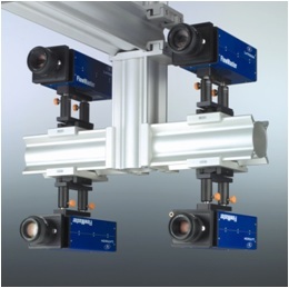
采用创新性的大尺度层析测量系统。用三台相机进行记录。得到在一个方形空气风洞中直径0.1m圆球体,在以1.45m/s平动时周围空间的3D3C速度矢量场,并根据这一矢量场结果,分析计算圆球的空气动力学阻力。
方案详情

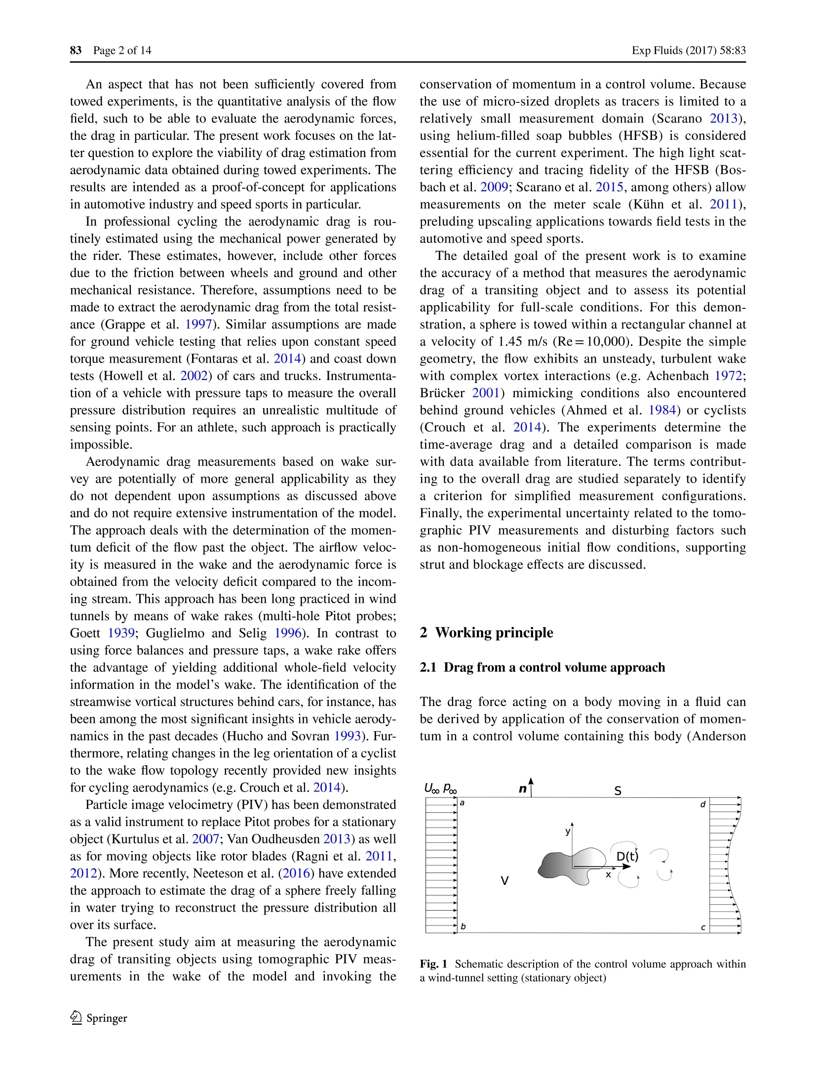
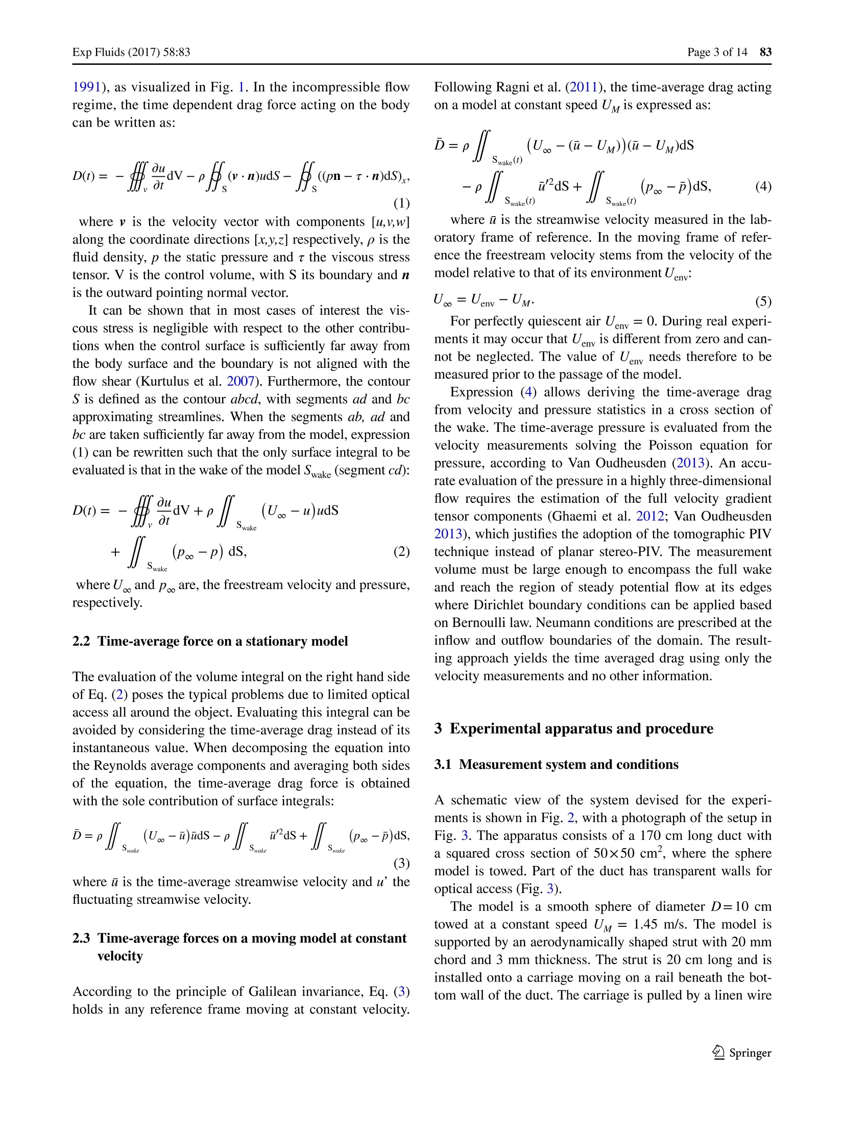
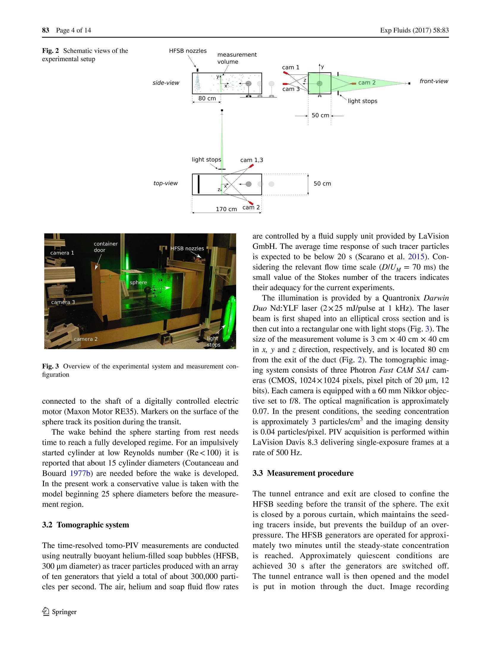
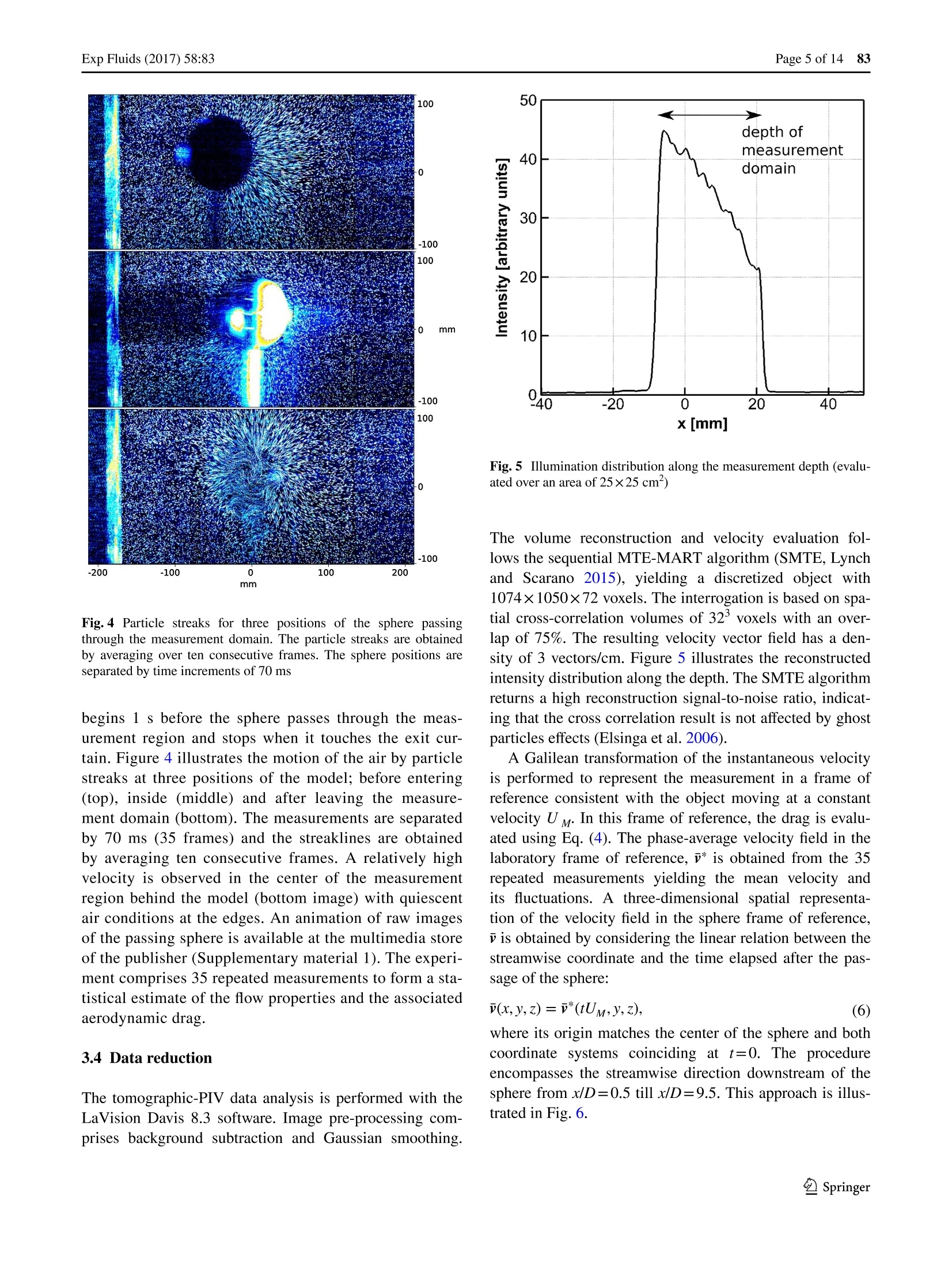
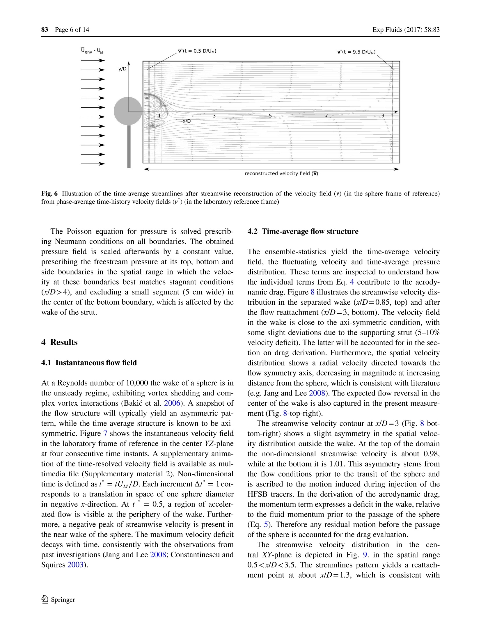
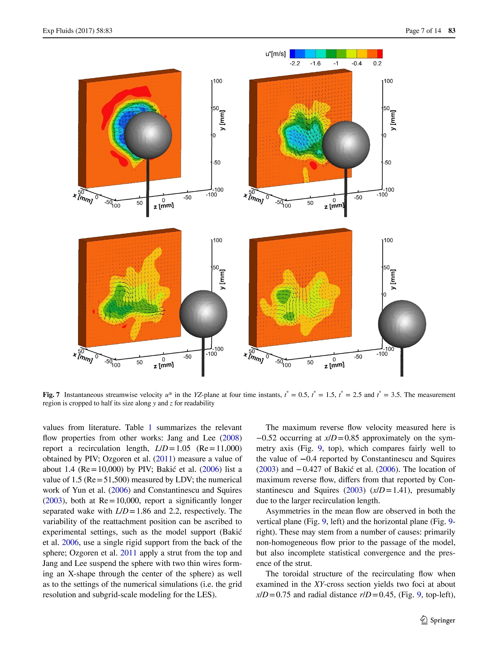
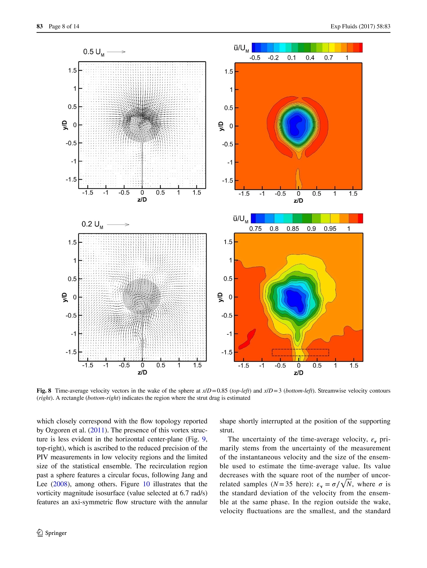
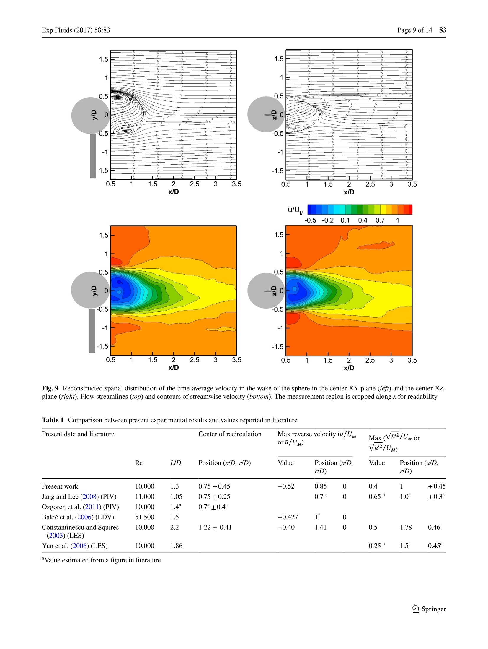
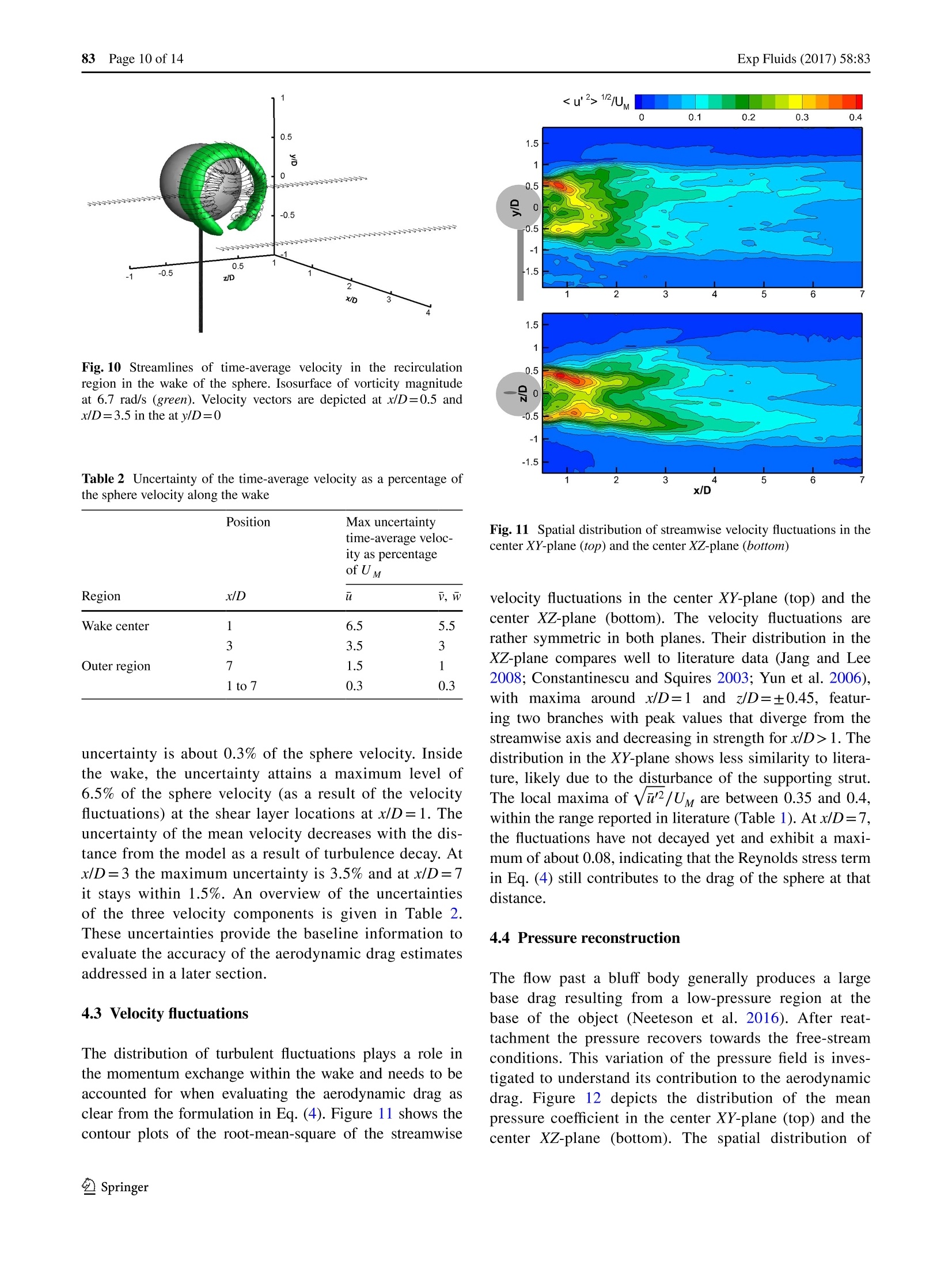
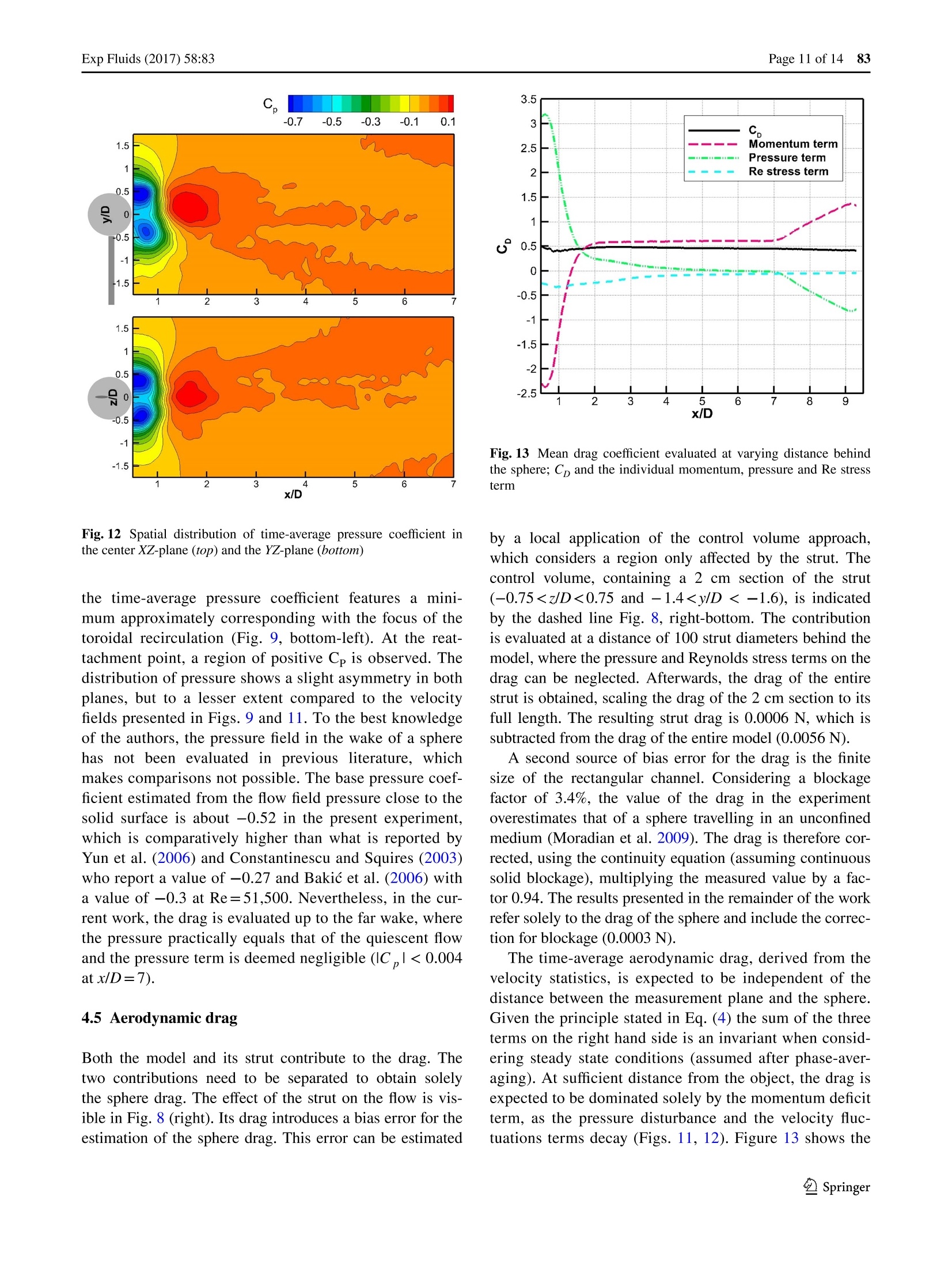
Exp Fluids (2017)58:83DOI 10.1007/s00348-017-2331-0CrossMark 83 Page 2 of 14Exp Fluids (2017) 58:83 Aerodynamic drag ofa transiting sphere by large-scaletomographic-PIV W. Terral· A. Sciacchitanol·F. Scarano AbstracttAA method is introduced to measure the aero-dynamic drag of moving objects such as ground vehiclesor athletes in speed sports. Experiments are conductedas proof-of-concept that yield the aerodynamic drag ofa sphere towed through a square duct in stagnant air. Thedrag force is evaluated using large-scale tomographic PIVand invoking the time-average momentum equation withina control volume in a frame of reference moving with theobject. The sphere with 0.1 m diameter moves at a veloc-ity of 1.45 m/s, corresponding to a Reynolds number of10,000. The measurements in the wake of the sphere areconducted at a rate of 500 Hz within a thin volume ofapproximately 3×40×40 cubic centimeters. Neutrallybuoyant helium-filled soap bubbles are used as flow trac-ers. The terms composing the drag are related to the flowmomentum, the pressure and the velocity fluctuations andthey are separately evaluated. The momentum and pressureterms dominate the momentum budget in the near wakeup to 1.3 diameters downstream of the model. The pres-sure term decays rapidly and vanishes within 5 diameters.The term due to velocity fluctuations contributes up to10% to the drag. The measurements yield a relatively con-stant value of the drag coefficient starting from 2 diametersdownstream of the sphere. At 7 diameters the measurementinterval terminates due to the finite length of the duct. Errorsources that need to be accounted for are the sphere support Electronic supplementary material The online version of thisarticle (doi:10.1007/s00348-017-2331-0) contains supplementarymaterial, which is available to authorized users. ( 区 W. Terraw.terra@tudelft.nl ) ( Aerospace Engineering Department, TU De l ft, Delft, The Netherlands ) wake and blockage effects. The above findings can providepractical criteria for the drag evaluation of generic bluffobjects with this measurement technique. Keywords Tomographic PIV ·Momentum equation .Aerodynamic drag·HFSB·Sphere· Wake 1 Introduction Aerodynamic forces result from the relative motion of anobject in air. These forces are relevant for a multitude ofapplications, such as aircraft systems, wind turbines andground transportation. Aerodynamic forces are typicallymeasured by means of wind tunnel experiments (Baconand Reid 1924; Zdravkovich 1990 among others), wherethe model is immersed in a uniform air stream within accu-rately controlled conditions. In other cases, aerodynamicstudies are conducted with the object moving in a quies-cent fluid. This approach is needed for instance to study theflow behind accelerating objects (Coutanceau and Bouard1977a) or the development of the wake of an aircraft overa large distance (Scarano et al. 2002; Von Carmer et al.2008). Furthermore, instructive flow visualizations havebeen obtained of high-speed flight of a bullet in stagnant air(van Dyke 1982). Aerodynamic investigations for groundvehicles and speed sports such as cycling, skating and ski-ing require specific arrangements of the wind tunnel (mov-ing floor, model supports) to achieve realistic conditions.Yet, experiments that simulate specific conditions suchas curved trajectories, acceleration, or with the athlete inmotion remain challenging. In contrast, experiments con-ducted with the object moving in the laboratory frame ofreference are relatively easy to realize and can mimic moreclosely real-life conditions. An aspect that has not been sufficiently covered fromtowed experiments, is the quantitative analysis of the flowfield, such to be able to evaluate the aerodynamic forces,the drag in particular. The present work focuses on the lat-ter question to explore the viability of drag estimation fromaerodynamic data obtained during towed experiments. Theresults are intended as a proof-of-concept for applicationsin automotive industry and speed sports in particular. In professional cycling the aerodynamic drag is rou-tinely estimated using the mechanical power generated bythe rider. These estimates, however, include other forcesdue to the friction between wheels and ground and othermechanical resistance. Therefore, assumptions need to bemade to extract the aerodynamic drag from the total resist-ance (Grappe et al. 1997). Similar assumptions are madefor ground vehicle testing that relies upon constant speedtorque measurement (Fontaras et al. 2014) and coast downtests (Howell et al. 2002) of cars and trucks. Instrumenta-tion of a vehicle with pressure taps to measure the overallpressure distribution requires an unrealistic multitude ofsensing points. For an athlete, such approach is practicallyimpossible Aerodynamic drag measurements based on wake survey are potentially of more general applicability as theydo not dependent upon assumptions as discussed aboveand do not require extensive instrumentation of the model.The approach deals with the determination of the momen-tum deficit of the flow past the object. The airflow veloc-ity is measured in the wake and the aerodynamic force isobtained from the velocity deficit compared to the incom-ing stream. This approach has been long practiced in windtunnels by means of wake rakes (multi-hole Pitot probes;Goett 1939; Guglielmo and Selig 1996). In contrast tousing force balances and pressure taps, a wake rake offersthe advantage of yielding additional whole-field velocityinformation in the model’s wake. The identification of thestreamwise vortical structures behind cars, for instance, hasbeen among the most significant insights in vehicle aerody-namics in the past decades (Hucho and Sovran 1993). Fur-thermore, relating changes in the leg orientation of a cyclistto the wake flow topology recently provided new insightsfor cycling aerodynamics (e.g.Crouch et al. 2014). Particle image velocimetry (PIV) has been demonstratedas a valid instrument to replace Pitot probes for a stationaryobject (Kurtulus et al. 2007; Van Oudheusden 2013) as wellas for moving objects like rotor blades (Ragni et al. 2011,2012). More recently, Neeteson et al. (2016) have extendedthe approach to estimate the drag of a sphere freely fallingin water trying to reconstruct the pressure distribution allover its surface. The present study aim at measuring the aerodynamicdrag of transiting objects using tomographic PIV meas-urements in the wake of the model and invoking the conservation of momentum in a control volume. Becausethe use of micro-sized droplets as tracers is limited to arelatively small measurement domain (Scarano 2013),using helium-filled soap bubbles (HFSB) is consideredessential for the current experiment. The high light scat-tering efficiency and tracing fidelity of the HFSB (Bos-bach et al. 2009; Scarano et al. 2015, among others) allowmeasurements on the meter scale (Kiihn et al. 2011),preluding upscaling applications towards field tests in theautomotive and speed sports. The detailed goal of the present work is to examinethe accuracy of a method that measures the aerodynamicdrag of a transiting object and to assess its potentialapplicability for full-scale conditions. For this demon-stration, a sphere is towed within a rectangular channel ata velocity of 1.45 m/s (Re=10,000). Despite the simplegeometry, the flow exhibits an unsteady, turbulent wakewith complex vortex interactions (e.g. Achenbach 1972;Brucker 2001) mimicking conditions also encounteredbehind ground vehicles (Ahmed et al. 1984) or cyclists(Crouch et al. 2014). The experiments determine thetime-average drag and a detailed comparison is madewith data available from literature. The terms contribut-ing to the overall drag are studied separately to identifya criterion for simplified measurement configurations.Finally, the experimental uncertainty related to the tomo-graphic PIV measurements and disturbing factors suchas non-homogeneous initial flow conditions, supportingstrut and blockage effects are discussed. 2 Working principle 2.1 Drag from a control volume approach The drag force acting on a body moving in a fluid canbe derived by application of the conservation of momen-tum in a control volume containing this body (Anderson Fig.1 Schematic description of the control volume approach withina wind-tunnel setting (stationary object) 1991), as visualized in Fig. 1. In the incompressible flowregime, the time dependent drag force acting on the bodycan be written as: where v is the velocity vector with components [u,y,w]along the coordinate directions [x,y,z] respectively, p is thefluid density, p the static pressure and t the viscous stresstensor. V is the control volume, with S its boundary and nis the outward pointing normal vector. It can be shown that in most cases of interest the vis-cous stress is negligible with respect to the other contributions when the control surface is sufficiently far away fromthe body surface and the boundary is not aligned with theflow shear (Kurtulus et al. 2007). Furthermore, the contourS is defined as the contour abcd, with segments ad and bcapproximating streamlines. When the segments ab, ad andbc are taken sufficiently far away from the model, expression(1) can be rewritten such that the only surface integral to beevaluated is that in the wake of the model Swake (segment cd): where Uand p are, the freestream velocity and pressure,respectively. 2.2 Time-average force on a stationary model The evaluation of the volume integral on the right hand sideof Eq. (2) poses the typical problems due to limited opticalaccess all around the object. Evaluating this integral can beavoided by considering the time-average drag instead of itsinstantaneous value. When decomposing the equation intothe Reynolds average components and averaging both sidesof the equation, the time-average drag force is obtainedwith the sole contribution of surface integrals: (3) where u is the time-average streamwise velocity and u’ thefluctuating streamwise velocity 2.3 Time-average forces on a moving model at constantvelocity According to the principle of Galilean invariance, Eq. (3)holds in any reference frame moving at constant velocity. Following Ragni et al. (2011), the time-average drag actingon a model at constant speed UM is expressed as: where u is the streamwise velocity measured in the lab-oratory frame of reference. In the moving frame of refer-ence the freestream velocity stems from the velocity of themodel relative to that of its environment Ueny: For perfectly quiescent air Ueny=0.During real experi-ments it may occur that Ueny is different from zero and can-not be neglected. The value of Ueny needs therefore to bemeasured prior to the passage of the model. Expression (4) allows deriving the time-average dragfrom velocity and pressure statistics in a cross section ofthe wake. The time-average pressure is evaluated from thevelocity measurements solving the Poisson equation forpressure, according to Van Oudheusden (2013). An accu-rate evaluation of the pressure in a highly three-dimensionalflow requires the estimation of the full velocity gradienttensor components (Ghaemi et al. 2012; Van Oudheusden2013), which justifies the adoption of the tomographic PIVtechnique instead of planar stereo-PIV. The measurementvolume must be large enough to encompass the full wakeand reach the region of steady potential flow at its edgeswhere Dirichlet boundary conditions can be applied basedon Bernoulli law. Neumann conditions are prescribed at theinflow and outflow boundaries of the domain. The result-ing approach yields the time averaged drag using only thevelocity measurements and no other information. 3 Experimental apparatus and procedure 3.1 Measurement system and conditions A schematic view of the system devised for the experi-ments is shown in Fig. 2, with a photograph of the setup inFig. 3. The apparatus consists of a 170 cm long duct witha squared cross section of 50×50 cm, where the spheremodel is towed. Part of the duct has transparent walls foroptical access (Fig. 3). The model is a smooth sphere of diameter D=10 cmtowed at a constant speed UM = 1.45 m/s. The model issupported by an aerodynamically shaped strut with 20 mmchord and 3 mm thickness. The strut is 20 cm long and isinstalled onto a carriage moving on a rail beneath the bot-tom wall of the duct. The carriage is pulled by a linen wire experimental setup front-view Fig. 3 Overview of the experimental system and measurement con-figuration connected to the shaft of a digitally controlled electricmotor (Maxon Motor RE35). Markers on the surface of thesphere track its position during the transit. The wake behind the sphere starting from rest needstime to reach a fully developed regime. For an impulsivelystarted cylinder at low Reynolds number (Re<100) it isreported that about 15 cylinder diameters (Coutanceau andBouard 1977b) are needed before the wake is developed.In the present work a conservative value is taken with themodel beginning 25 sphere diameters before the measure-ment region. 3.2 Tomographic system The time-resolved tomo-PIV measurements are conductedusing neutrally buoyant helium-filled soap bubbles (HFSB,300 um diameter) as tracer particles produced with an arrayof ten generators that yield a total of about 300,000 parti-cles per second. The air, helium and soap fluid flow rates are controlled by a fluid supply unit provided by LaVisionGmbH. The average time response of such tracer particlesis expected to be below 20 s (Scarano et al. 2015). Con-sidering the relevant flow time scale (D/UM=70 ms) thesmall value of the Stokes number of the tracers indicatestheir adequacy for the current experiments. The illumination is provided by a Quantronix DarwinDuo Nd:YLF laser (2×25 mJ/pulse at 1 kHz). The laserbeam is first shaped into an elliptical cross section and isthen cut into a rectangular one with light stops (Fig.3). Thesize of the measurement volume is 3 cm × 40 cm × 40 cmin x, y and zdirection, respectively, and is located 80 cmfrom the exit of the duct (Fig. 2). The tomographic imag-ing system consists of three Photron Fast CAM SAl cam-eras (CMOS, 1024×1024 pixels, pixel pitch of 20 um, 12bits). Each camera is equipped with a 60 mm Nikkor objec-tive set to f/8. The optical magnification is approximately0.07. In the present conditions, the seeding concentrationis approximately 3 particles/cm’and the imaging densityis 0.04 particles/pixel. PIV acquisition is performed withinLaVision Davis 8.3 delivering single-exposure frames at arate of 500 Hz. 3.3 Measurement procedure The tunnel entrance and exit are closed to confine theHFSB seeding before the transit of the sphere. The exitis closed by a porous curtain, which maintains the seed-ing tracers inside, but prevents the buildup of an over-pressure. The HFSB generators are operated for approxi-mately two minutes until the steady-state concentrationiSIreached. Approximately quiescent conditionsareachieved 30 s after the generators are switched off.The tunnel entrance wall is then opened and the modelis put in motion through the duct. Image recording Fig. 4 Particle streaks for three positions of the sphere passingthrough the measurement domain. The particle streaks are obtainedby averaging over ten consecutive frames.The sphere positions areseparated by time increments of 70 ms begins 1 s before the sphere passes through the meas-urement region and stops when it touches the exit cur-tain. Figure 4 illustrates the motion of the air by particlestreaks at three positions of the model; before entering(top), inside (middle) and after leaving the measure-ment domain (bottom). The measurements are separatedby 70 ms (35 frames) and the streaklines are obtainedby averaging ten consecutive frames. A relatively highvelocity is observed in the center of the measurementregion behind the model (bottom image) with quiescentair conditions at the edges. An animation of raw imagesof the passing sphere is available at the multimedia storeof the publisher (Supplementary material 1). The experi-ment comprises 35 repeated measurements to form a sta-tistical estimate of the flow properties and the associatedaerodynamic drag. 3.4 Data reduction The tomographic-PIV data analysis is performed with theLaVision Davis 8.3 software. Image pre-processing com-prises background subtraction and Gaussian smoothing. Fig.5 Illumination distribution along the measurement depth (evalu-ated over an area of 25×25cm) The volume reconstruction and velocity evaluation fol-lows the sequential MTE-MART algorithm (SMTE, Lynchand Scarano 2015), yielding a discretized object with1074×1050×72 voxels. The interrogation is based on spa-tial cross-correlation volumes of 32’ voxels with an over-lap of 75%. The resulting velocity vector field has a den-sity of 3 vectors/cm. Figure 5 illustrates the reconstructedintensity distribution along the depth. The SMTE algorithmreturns a high reconstruction signal-to-noise ratio, indicat-ing that the cross correlation result is not affected by ghostparticles effects (Elsinga et al. 2006). A Galilean transformation of the instantaneous velocityis performed to represent the measurement in a frame ofreference consistent with the object moving at a constantvelocity U M. In this frame of reference, the drag is evalu-ated using Eq. (4). The phase-average velocity field in thelaboratory frame of reference, v* is obtained from the 35repeated measurements yielding the mean velocity andits fluctuations. A three-dimensional spatial representa-tion of the velocity field in the sphere frame of reference,y is obtained by considering the linear relation between thestreamwise coordinate and the time elapsed after the pas-sage of the sphere: where its origin matches the center of the sphere and bothcoordinate systems coinciding at t=0. The procedureencompasses the streamwise direction downstream of thesphere from x/D=0.5 till x/D=9.5. This approach is illus-trated in Fig. 6. reconstructed velocity field (v) Fig. 6 Illustration of the time-average streamlines after streamwise reconstruction of the velocity field (v) (in the sphere frame of reference)from phase-average time-history velocity fields (v") (in the laboratory reference frame) The Poisson equation for pressure is solved prescrib-ing Neumann conditions on all boundaries. The obtainedpressure field is scaled afterwards by a constant value,prescribing the freestream pressure at its top, bottom andside boundaries in the spatial range in which the veloc-ity at these boundaries best matches stagnant conditions(x/D>4), and excluding a small segment (5 cm wide) inthe center of the bottom boundary, which is affected by thewake of the strut. 4 Results 4.1 Instantaneous flow field At a Reynolds number of 10,000 the wake of a sphere is inthe unsteady regime, exhibiting vortex shedding and com-plex vortex interactions (Bakic et al. 2006). A snapshot ofthe flow structure will typically yield an asymmetric pat-tern, while the time-average structure is known to be axi-symmetric. Figure 7 shows the instantaneous velocity fieldin the laboratory frame of reference in the center YZ-planeat four consecutive time instants. A supplementary anima-tion of the time-resolved velocity field is available as mul-timedia file (Supplementary material 2). Non-dimensionaltime is defined as t"=tUM/D. Each increment △t*=1 cor-responds to a translation in space of one sphere diameterin negative x-direction. At t *=0.5, a region of acceler-ated flow is visible at the periphery of the wake. Further-more, a negative peak of streamwise velocity is present inthe near wake of the sphere. The maximum velocity deficitdecays with time, consistently with the observations frompast investigations (Jang and Lee 2008; Constantinescu andSquires 2003). 4.2 Time-average flow structure The ensemble-statistics yield the time-average velocityfield, the fluctuating velocity and time-average pressuredistribution. These terms are inspected to understand howthe individual terms from Eq. 4 contribute to the aerody-namic drag. Figure 8 illustrates the streamwise velocity dis-tribution in the separated wake (x/D=0.85, top) and afterthe flow reattachment (x/D=3, bottom). The velocity fieldin the wake is close to the axi-symmetric condition, withsome slight deviations due to the supporting strut (5-10%velocity deficit). The latter will be accounted for in the sec-tion on drag derivation. Furthermore, the spatial velocitydistribution shows a radial velocity directed towards theflow symmetry axis, decreasing in magnitude at increasingdistance from the sphere, which is consistent with literature(e.g. Jang and Lee 2008). The expected flow reversal in thecenter of the wake is also captured in the present measure-ment (Fig. 8-top-right). The streamwise velocity contour at x/D=3 (Fig. 8 bot-tom-right) shows a slight asymmetry in the spatial veloc-ity distribution outside the wake. At the top of the domainthe non-dimensional streamwise velocity is about 0.98,while at the bottom it is 1.01. This asymmetry stems fromthe flow conditions prior to the transit of the sphere andis ascribed to the motion induced during injection of theHFSB tracers. In the derivation of the aerodynamic drag,the momentum term expresses a deficit in the wake, relativeto the fluid momentum prior to the passage of the sphere(Eq. 5). Therefore any residual motion before the passageof the sphere is accounted for the drag evaluation. The streamwise velocity distributioninintthecen-tral XY-plane is depicted in Fig. 9. in the spatial range0.5 1. Thedistribution in the XY-plane shows less similarity to litera-ture, likely due to the disturbance of the supporting strut.The local maxima of √ur/Um are between 0.35 and 0.4,within the range reported in literature (Table 1). At x/D=7,the fluctuations have not decayed yet and exhibit a maxi-mum of about 0.08, indicating that the Reynolds stress termin Eq. (4) still contributes to the drag of the sphere at thatdistance. 4.4 Pressure reconstruction The flow past a bluff body generally produces a largebase drag resulting from a low-pressure region at thebase of the object (Neeteson et al.2016). After reat-tachment the pressure recovers towards the free-streamconditions. This variation of the pressure field is inves-tigated to understand its contribution to the aerodynamicdrag. Figure 12 depicts the distribution of the meanpressure coefficient in the center XY-plane (top) and thecenter XZ-plane (bottom). The spatial distribution of Fig. 12 Spatial distribution of time-average pressure coefficient inthe center XZ-plane (top) and the YZ-plane (bottom) the time-average pressure coefficient features a mini-mum approximately corresponding with the focus of thetoroidal recirculation (Fig. 9, bottom-left). At the reat-tachment point, a region of positive Cp is observed. Thedistribution of pressure shows a slight asymmetry in bothplanes, but to a lesser extent compared to the velocityfields presented in Figs. 9 and 11. To the best knowledgeof the authors, the pressure field in the wake of a spherehas not been evaluated in previous literature, whichmakes comparisons not possible. The base pressure coef-ficient estimated from the flow field pressure close to thesolid surface is about -0.52 in the present experiment,which is comparatively higher than what is reported byYun et al. (2006) and Constantinescu and Squires (2003)who report a value of -0.27 and Bakic et al. (2006) witha value of -0.3 at Re=51,500. Nevertheless, in the cur-rent work, the drag is evaluated up to the far wake, wherethe pressure practically equals that of the quiescent flowand the pressure term is deemed negligible (IC,l<0.004at x/D=7). 4.5 Aerodynamic drag Both the model and its strut contribute to the drag. Thetwo contributions need to be separated to obtain solelythe sphere drag. The effect of the strut on the flow is vis-ible in Fig. 8 (right). Its drag introduces a bias error for theestimation of the sphere drag. This error can be estimated Fig. 13 Mean drag coefficient evaluated at varying distance behindthe sphere; Cp and the individual momentum, pressure and Re stressterm by a local application of the control volume approach,which considers a region only affected by the strut. Thecontrol volume, containing a 2 cm section of the strut(-0.752. The statistical uncertainty of the mean drag coefficient,ec N mostly stems from variations in the instantane-ous drag, caused by large scale fluctuations in the wake.It scales inversely proportional to √N, where N is thestatistical ensemble size. The latter can be enlarged byincreasing the number of passages of the sphere Np, andthe amount of uncorrelated stations selected along thewake Ns: In the present experiments the statistical ensemble isbuilt from 35 individual passages (Np = 35) of the sphereand three stations x/D={5,6,7} in the wake (Ns=3), inthe range where the pressure term can be neglected. Con-sidering that the uncertainty of the drag coefficient from asingle sample is e N to 0.26, the above condition reducethe statistical uncertainty to approximately ec N to 0.026 at95% coverage factor. Any further decrease of the uncertainty of the meandrag coefficient relies on the increase of N p and N s. Forthe latter,the assumption of negligible environmental dis-turbances during the observation time must hold true.This means that after the passage of the model through themeasurement region, momentum is not added by externalsources or removed for instance due to wall interactions. Considering the latter uncertainty, the presented valuefor the drag coefficient of 0.47 falls within the range ofreported values in literature: Moradian et al. (2009) meas-ured a Cp of about 0.51 (Re=22,000) by load cells, Achen-bach (1972), a value of 0.5 (Re=60,000) by strain gauges,while Constantinescu and Squires (2003) and Yun et al.(2006) report a value of 0.39 (Re=10,000). Finally, regarding the applicability of the control volumeapproach to other bluff body flows, it is worth mentioningthat the flow over spheres becomes turbulent at a Reynoldsnumber around 800 and remains so afterwards. Hence, thestatistical approach to determine the drag can be consideredalso for experiments at a higher Reynolds number. There-fore, the conclusions drawn from this study can be extrapo-lated to model geometries other than the sphere under theassumption of similarity in the behavior of the wake 5 Conclusions Time resolved tomographic-PIV measurements are con-ducted to determine the aerodynamic drag of a transitingsphere using the control volume approach in the wake of the model. The concept is demonstrated using a newlydeveloped system to measure the flow over a sphere witha diameter of 10 cm moving at 1.45 m/s. Velocity statis-tics in the wake of the sphere have been obtained from aset of 35 model transits. The obtained time-average veloc-ity and its fluctuations are used to estimate the flow fieldpressure. The aerodynamic drag is evaluated via a controlvolume approach as the sum of these three contributionsalong the wake behind the sphere. The estimation of thedrag coefficient is practically unaffected by the positionwhere the momentum integral is evaluated. In particular,the time-average drag coefficient obtained 2 sphere diam-eters behind the model falls within the range of reportedvalues in literature. For practical applications of this approach, it is observedthat the pressure term vanishes after 5 diameters, which cangreatly simplify the measurement procedure. Three disturb-ing factors are worth mentioning that may affect the meas-urement accuracy: the flow conditions prior to the passageof the sphere need to be taken into account in the evalu-ation; the blockage effect due to the finite channel crosssection; the contribution of the supporting strut needs to besubtracted to isolate that of the main object only. Acknowledgements This work is partly funded by the TU DelftSports Engineering Institute and the European Research CouncilProof of Concept Grant“Flow Visualization Based Pressure"(no.665477). Andrea Rubino is acknowledged for the support duringexperiments. Open Access This article is distributed under the terms of theCreative Commons Attribution 4.0 International License (http://creativecommons.org/licenses/by/4.0/), which permits unrestricteduse, distribution, and reproduction in any medium, provided you giveappropriate credit to the original author(s) and the source, provide alink to the Creative Commons license, and indicate if changes weremade. References Achenbach E (1972) Experiments on the flow past spheres at veryhigh Reynolds numbers. J Fluid Mech 54:565-575. doi:10.1017/SO022112072000874 ( Ahmed S R , R a mm G, F al t in G (19 8 4) Som e salient fea t ures ofthe time-averaged ground vehicl e wake . SAE Paper 840300.doi: 10.427 1 /840300 ) Anderson JD Jr (1991) Fundamentals of aerodynamics. Internationaledn.McGraw-Hill, New York Bacon DL, Reid EG (1924) The resistance of spheres in wind tunnelsand in air. NACA Annu Rep 9:469-487 Balachandar S, Mittal R, Najjar FM (1997) Properties of themean recirculation region in the wakes of two-dimensional ( bluff fHbodies. Jl Fluid d Mech 351:167-199. d doi: 10.1017/S00221 1 2097007179 ) ( Bosbach J , Kuhn M , Wagner C (2009) Large scale particle imagevelocimetry with h elium f illed s oap b ubbles. Exp Fluids46:539-547. doi: 10.1007/s00348-008-057 9 -0 ) ( Bricker C (2001) Spatio-temporal r e construction of vortex d ynam- i cs i n axisymmetric wakes. J Fluid Struct 15:543-554. doi:1 0. 1 006/jfls.2000.0356 ) ( Constantinesc u GS, Squire s KD (2003) LES a nd DES i n ves-tigations of turbulen t flo w ove r a spher e a t R e = 10,000.Flow T urb Comb 70:267-298. doi: 10.1023/B:APPL.0000004937.34078.71 ) ( Countanceau M, Bouard R (1977a) Experimental d etermination of the m ain features of the viscous f l ow i n t h e w a ke of a circu- lar cylinder i n uniform translation. Part 1. S teady f l ow. J FluidMech 79:231-256. doi: 10.10 1 7/S0022 112 077000135 ) ( Countanceau M ,B o uard R (1977b) E x perimental determination of the main features o f t he viscous f low i n the wake of a circular cylinder i n uniform t ranslation. Part 2. Unsteady flow. J Fluid Mech 79:257-272. doi: 1 0.1017/SO022 11 2077000147 ) ( Crouch TN, Burton D, Brown NAT, Thomson MC, Sheridan J (2014) Flow t o pology in the wake of a c y c list and it s e f fecton a erodynamic d r ag. J F l uid M e ch 74 8 :5-35. doi:10. 1017/ ifm . 2013.6 7 8 ) ( Elsinga GE, van Oudheusden B W, S c arano F ( 2 006) Experimentalassessment of tomographic-PIV a ccuracy. I n: 13th Int; Sympon A pplication of Laser Techniques to Fluid Dynamics, Lisbon, Portugal ) ( Fontaras G, Dilara P, B erner M, Volkers Te t a l. (2 0 14) An experi-mental m ethodology f o r measuring of aerodynamic re s istances of heavy duty vehicles in the framework of European CO, emis-sions monitoring scheme. SAE Int J Commer Veh 7: 1 02-110. doi: 10.427 1 /2014-01-0595 ) ( Ghaemi S , R a gni D , Scarano F ( 2 0 12) PI V -based pr e ssure fl u c-tuations in the turbulent boundary layer. Exp Fluids 53: 1 823.doi: 10.1007/s00348-012- 1 391 - 4 ) ( Goett HJ (1939) Experimental investigatio n of t h e momentum methodfor determining profile dra g . NACA Annu Rep 25:365-371. ) ( Grappe F, C andau R , B e lli A , R ouillon JD (1997) A erodynamic drag in f ield cycling with s pecial r eference to Obree’s position. Ergo- nomics 40:1299-1311. doi: 10 . 1080/00140 13 97187 3 88 ) ( Guglielmo JJ, S elig M S ( 1 996) Spanwise va r iations in profile d ragfor airfoil s a t low Reynolds n umbers. J A i rcr 33:699-707.doi: 10.2514/3.47004 ) ( Howell J, Sherwin C, Passmore M, Le Good G (2002) Aerody-namic drag of a compact SUV a s m easured on-Road and in the wind t unnel. SAE Technical Paper 2002-01-0529:583-590. doi: 10.427 1 /2002-01 - 0529 ) Hucho W, Sovran G (1993)3)Aerodynamics of roadd vehicles.Annu Rev Fluid Mech25:485-537. doi:10.1146/annurev.fl.25.010193.002413 ( Jang Y I , L ee SJ (2008) PIV a n alysis o f near-wake b e hind a sphereat a s ubcritica l Reynolds number. E xp F l uids 44:905-914.doi: 10.1007/s00348-007-0448-2 ) ( Kiihn M, Ehrenfried K, Bosbach J, W agner C (2 0 11) Large-scale tomographic p article image v elocimetry u sing h elium-fille d soap bubbles. Exp Fluids 5:0:929-948. d o i:10 .1007/s00348-010-0947-4 ) ( Kurtulus DF, Scarano F , D avid L ( 2 007) U n steady aerodynamic forces estimation on a square cylinder by TR-PIV. Exp Fluids 42:185-196. doi: 10 . 1007/s00348-006-02 2 8-4 ) ( Lynch K P , S c arano F ( 2015) An efficient and acc u rate approach toMTE-M A RT for time-resolved tomographic P IV. E xp Fluids56:66.doi: 10.1007/s00348-015- 1 934-6 ) ( Moradian N , Ting D SK, Cheng S (2009) The effects o f freestreamturbulence o n t he d r ag c o efficient of a s p here. E x p Th e rmal Fluid Sci 33:460-471. doi: 1 0. 1 016/j.exp t he r mflusci.2008 . 1 1 .001 ) ( Neeteson N J, B hattacharya S , R ival D E, Michaelis D , S c hanz D,Schroder A (2016) Pressure-field extraction from Lagrangianflow measurements: f irst experiences with 4D-PTV data. E xpFluids 57:102. doi : 10.1007/s00348-016-2170-4 ) ( Ozgoren M, Okbaz A, Kahraman A, Hassanzadeh R, Sahin B, AkilliH, D ogan S (2011) Ex p erimental Investigation of t he Flow struc-ture around a s p here and it s control w i th jet flow via PIV. In : 6th International Advanced Technologies Symposium,Elazig, Turkey ) ( Ragni D , v an Oudheusden BW, Scarano F ( 2011) Non-intrusive aero-dynamic loads analysis of an aircraft propeller blade. Exp Fluids51:361-371.doi: 1 0.1007/s00348-011-1057- 7 ) ( Ragni D , v an O udheusden BW, Sc a rano F (2012) 3D pressure imag- ing of a n aircraft p ropeller b lade-tip f low by phase-locked stereoscopic PIV.ExppFluids 52:463-477. doi: 1 0.1007/s00348-01 1 - 1236-6 ) ( Scarano F (2013) Tomographic PIV : principle and practice. Meas SciTechnol 24:012001. doi: 10.1088/0957-0233/24/1/012001 ) Scarano F, van Wijk C, Veldhuis LLM (2002) Traversing field of viewand AR-PIV for mid-field wake vortex investigation in a towingtank. Exp Fluids 33:950-961. doi:10.1007/s00348-002-0516-6 ( Scarano F, Ghaemi S, Caridi G CA, Bosbach J, Dierksheide U, Sciac- chitano A (2015) On t h e u s e o f helium-filled s oap bubbles f or large-scale tomographic PIV in w ind t u nnel experiments. E x p F luids 56:42. doi :10.1007/s00348-015-1909- 7 ) ( Van D yke M (1982) An album of fluid motion. The P a rabolic Press, Stanford ) Van Oudheusden BW (2013) PIV-based pressure measurement. MeasSci Technol 24 032001.doi:10.1088/0957-0233/24/3/032001 Von Carmer CF, Heider A, Schroder A, Konrath R, Agocs J, GilliotA, Monnier JC (2008) Evaluation of large-scale wing vortexwakes from multi-camera PIV measurements in free-flight labo-ratory.Part Image Velocim Top Appl Phys 112:377-394. Springer A method is introduced to measure the aerodynamicdrag of moving objects such as ground vehiclesor athletes in speed sports. Experiments are conductedas proof-of-concept that yield the aerodynamic drag ofa sphere towed through a square duct in stagnant air. Thedrag force is evaluated using large-scale tomographic PIVand invoking the time-average momentum equation withina control volume in a frame of reference moving with theobject. The sphere with 0.1 m diameter moves at a velocityof 1.45 m/s, corresponding to a Reynolds number of10,000. The measurements in the wake of the sphere areconducted at a rate of 500 Hz within a thin volume ofapproximately 3 × 40 × 40 cubic centimeters. Neutrallybuoyant helium-filled soap bubbles are used as flow tracers.The terms composing the drag are related to the flowmomentum, the pressure and the velocity fluctuations andthey are separately evaluated. The momentum and pressureterms dominate the momentum budget in the near wakeup to 1.3 diameters downstream of the model. The pressureterm decays rapidly and vanishes within 5 diameters.The term due to velocity fluctuations contributes up to10% to the drag. The measurements yield a relatively constantvalue of the drag coefficient starting from 2 diametersdownstream of the sphere. At 7 diameters the measurementinterval terminates due to the finite length of the duct. Errorsources that need to be accounted for are the sphere supportwake and blockage effects. The above findings can providepractical criteria for the drag evaluation of generic bluffobjects with this measurement technique.
确定
还剩12页未读,是否继续阅读?

产品配置单


北京欧兰科技发展有限公司为您提供《平移运动球体中空气动力学阻力,3D3C速度场检测方案(粒子图像测速)》,该方案主要用于其他中空气动力学阻力,3D3C速度场检测,参考标准--,《平移运动球体中空气动力学阻力,3D3C速度场检测方案(粒子图像测速)》用到的仪器有体视层析粒子成像测速系统(Tomo-PIV)、LaVision DaVis 智能成像软件平台
推荐专场


相关方案
更多
该厂商其他方案
更多