


方案详情
文
层析-PIV,Tomo-PIV是德国LaVision公司独有的能够测量获得高分辨率全体积3分量速度矢量场的系统。本篇介绍了先进的运动追踪增强粒子重构算法MTE-MART的原理和应用。采用这种算法,在相同的硬件配置下,可以处理更高浓度的粒子场,得到空间分辨率更高的速度矢量场。
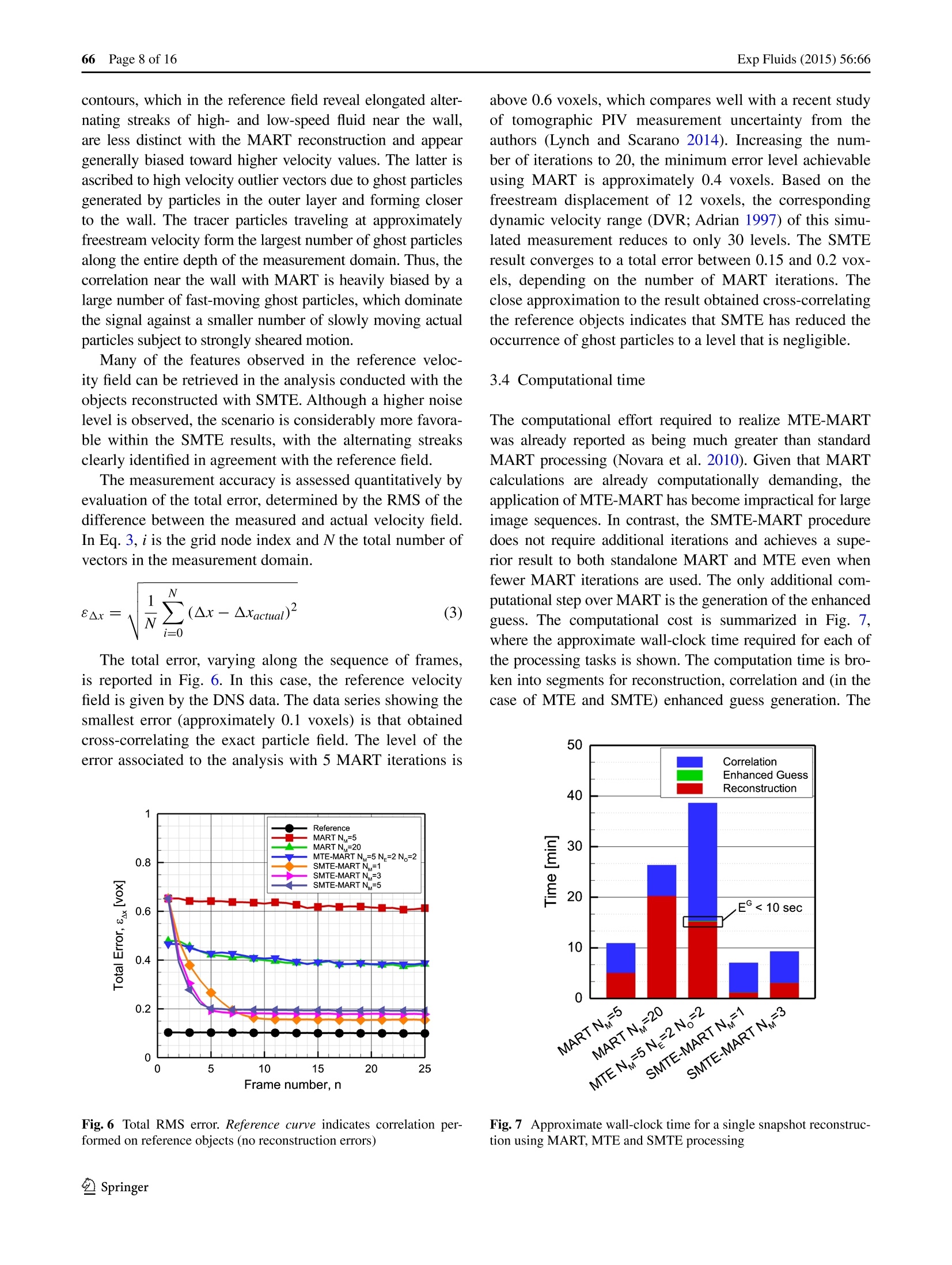
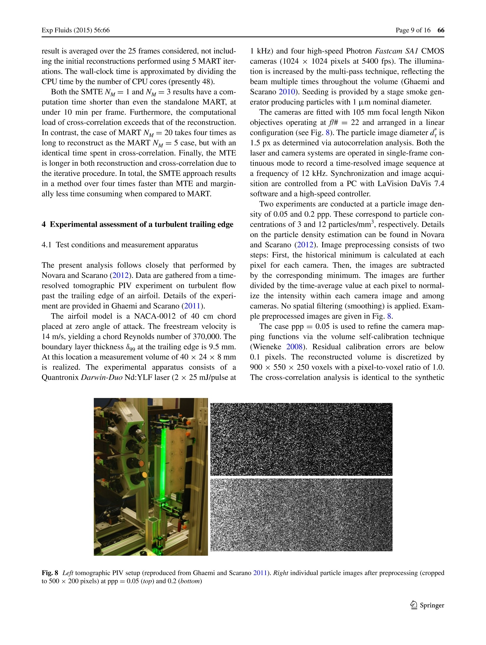
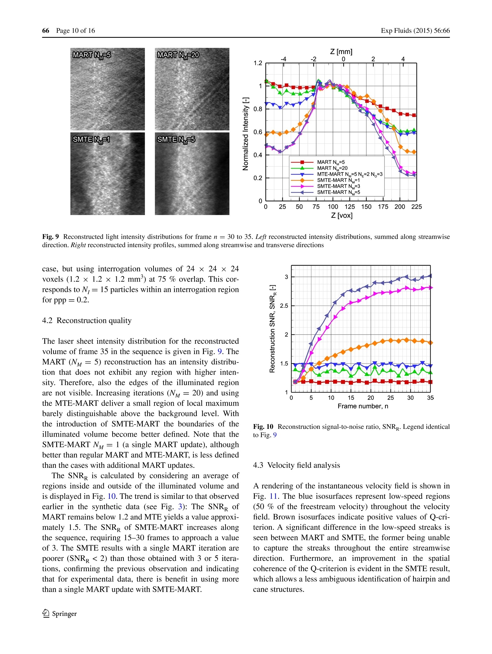
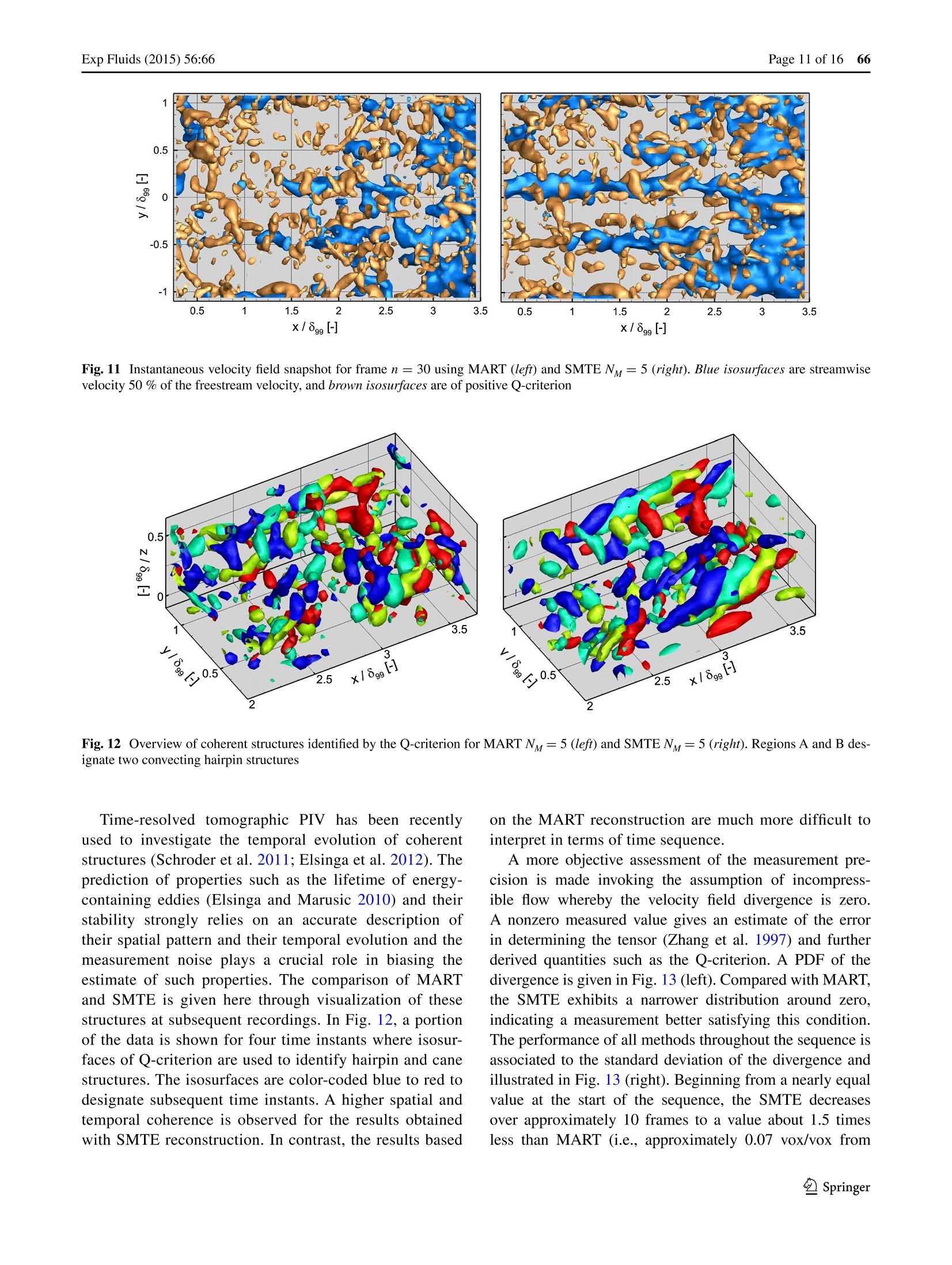
方案详情

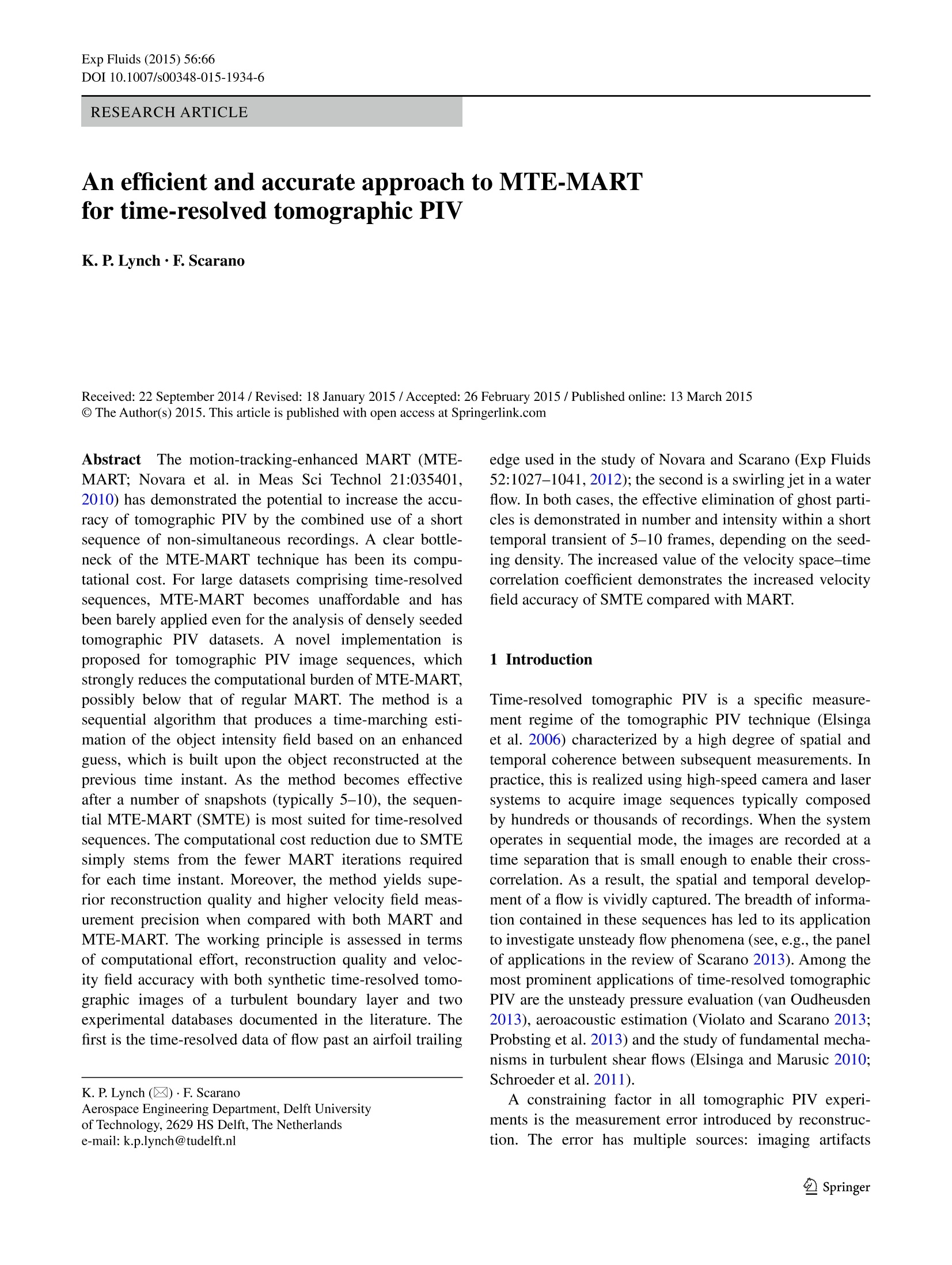
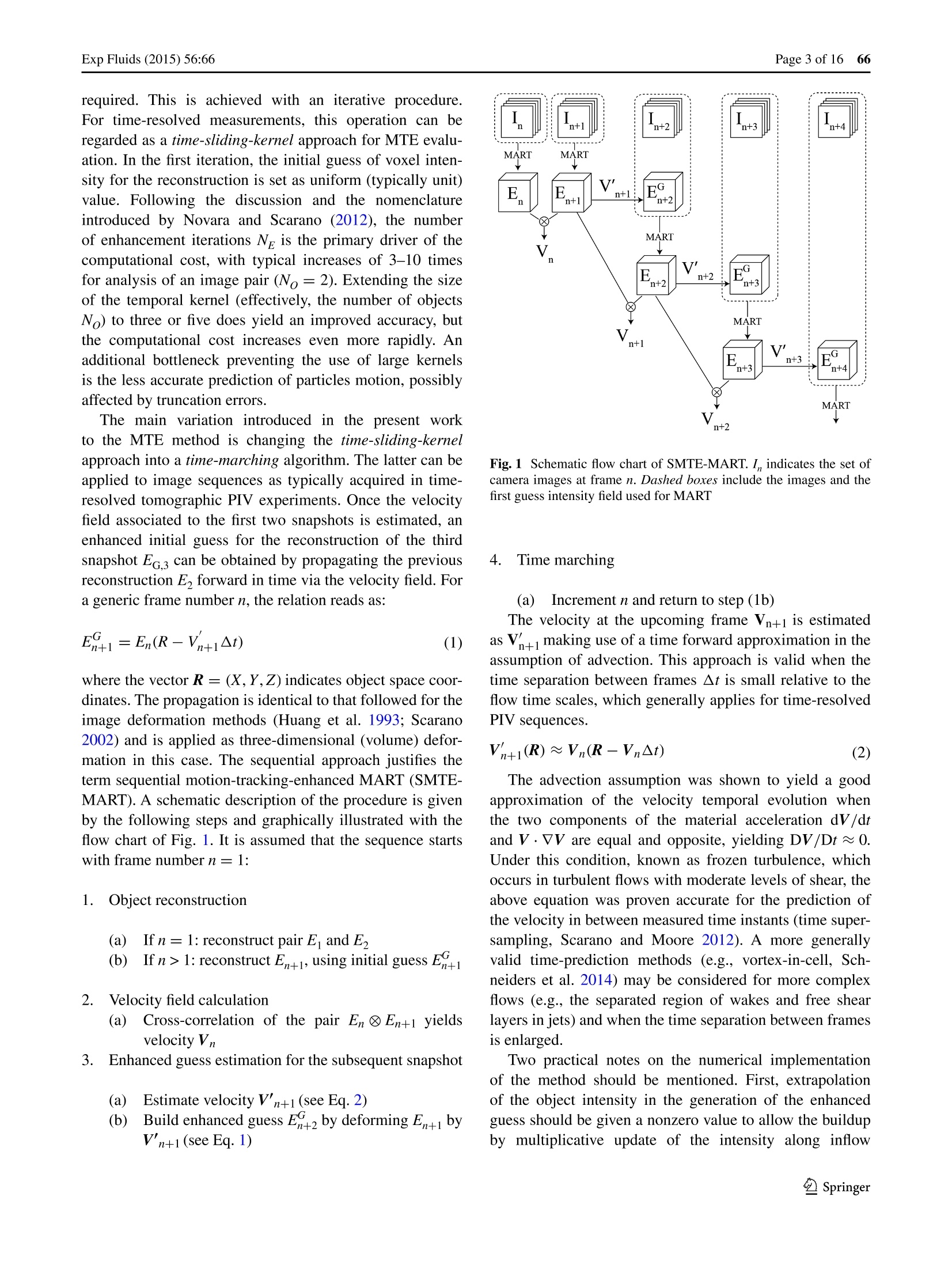
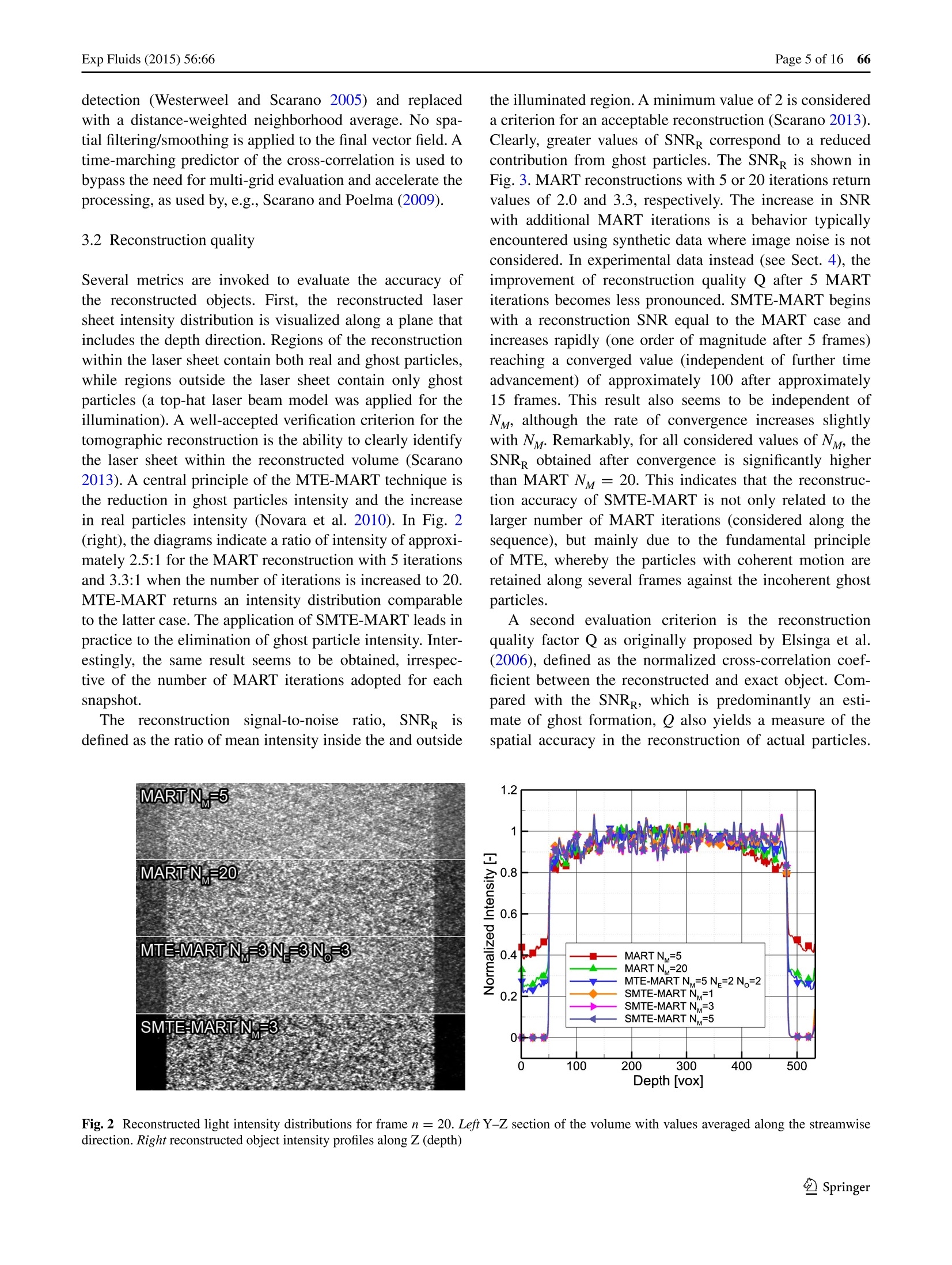
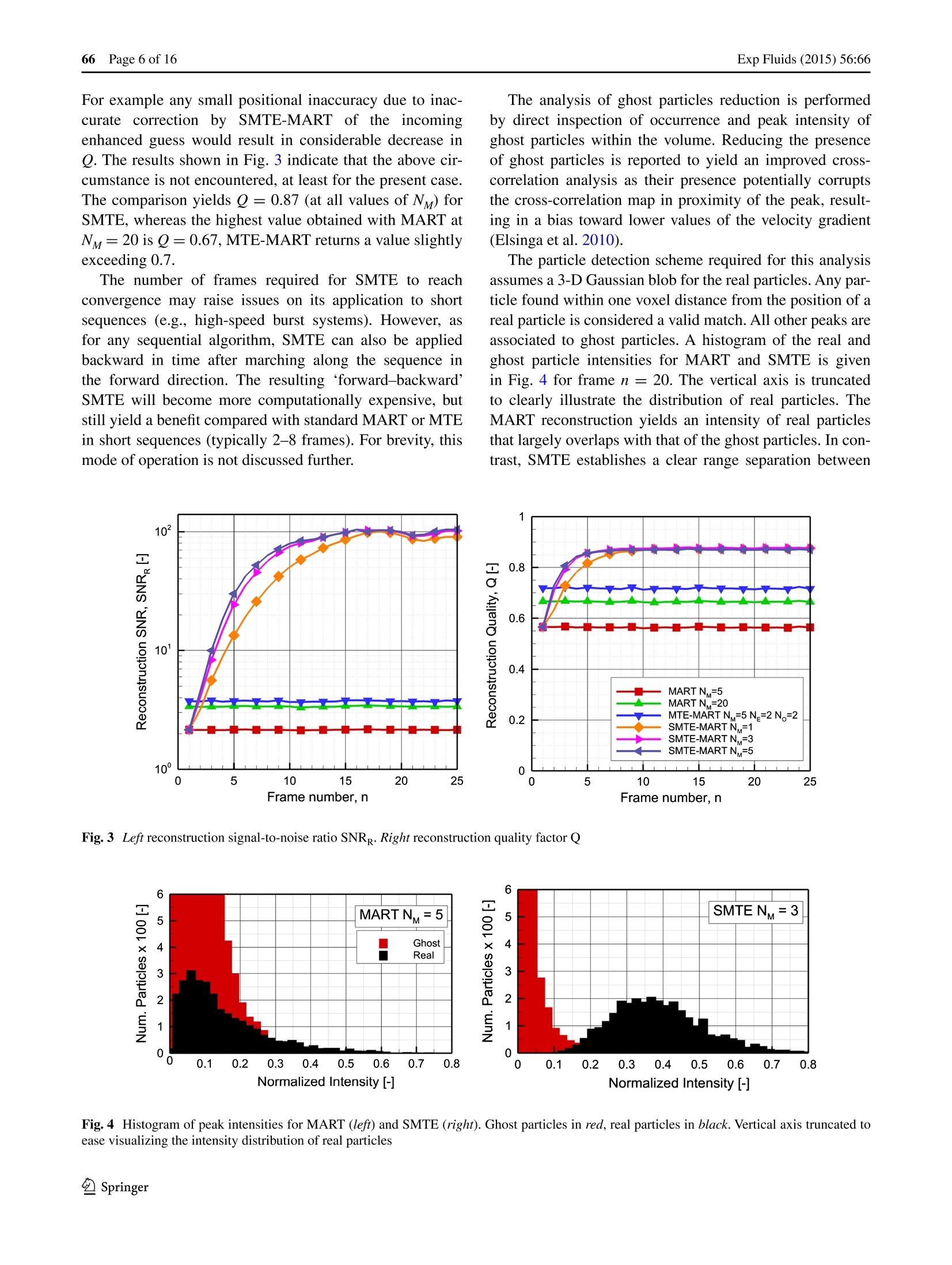
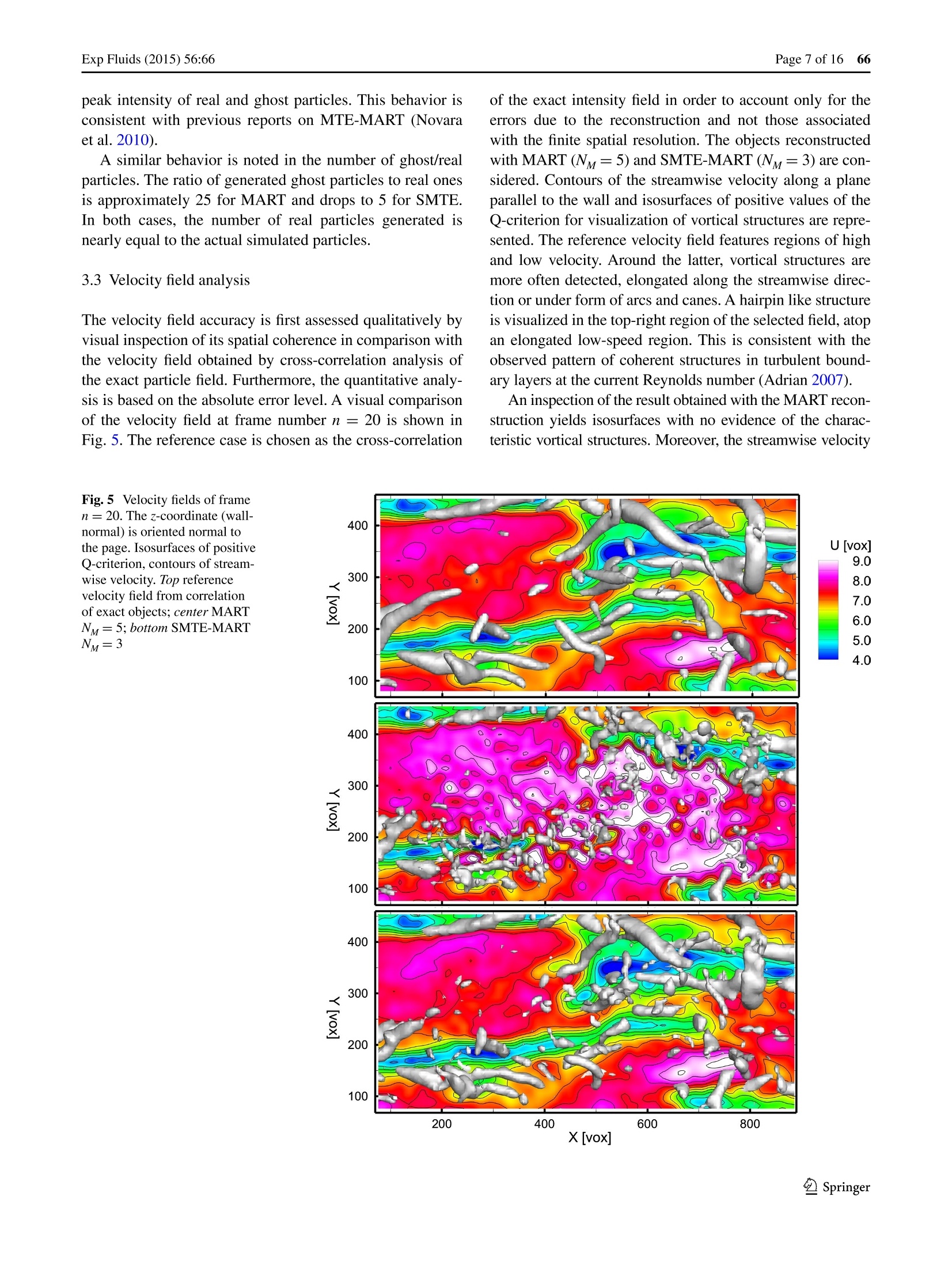
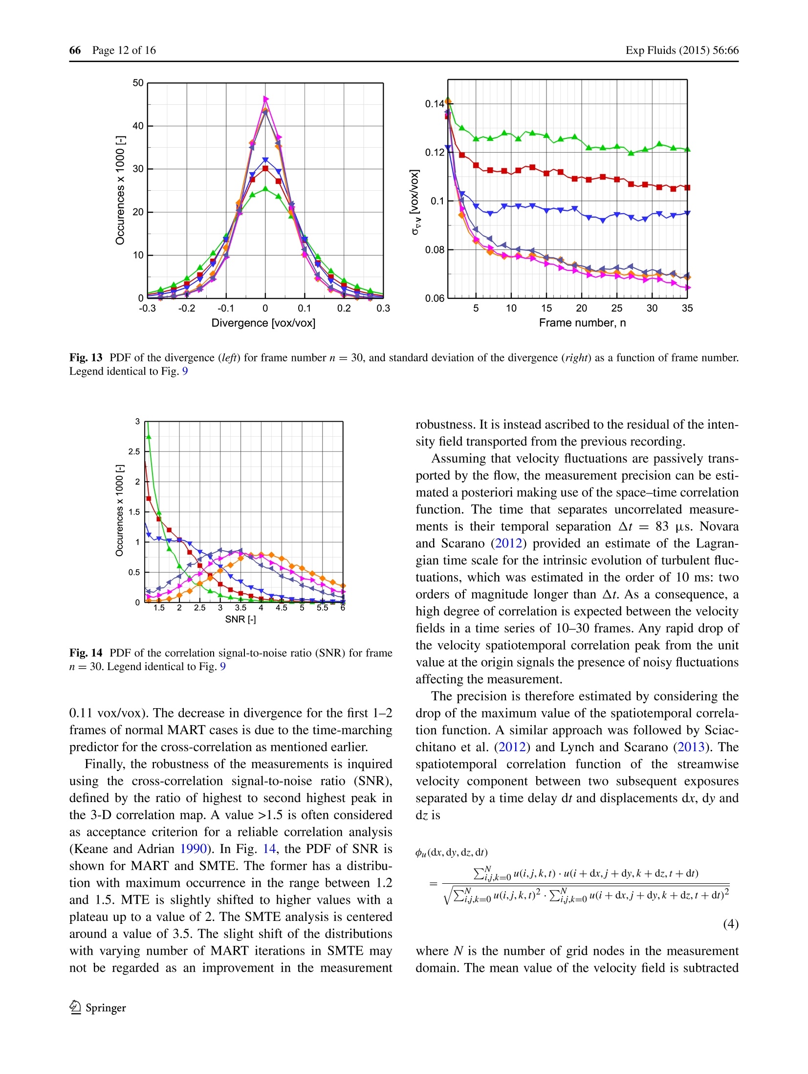
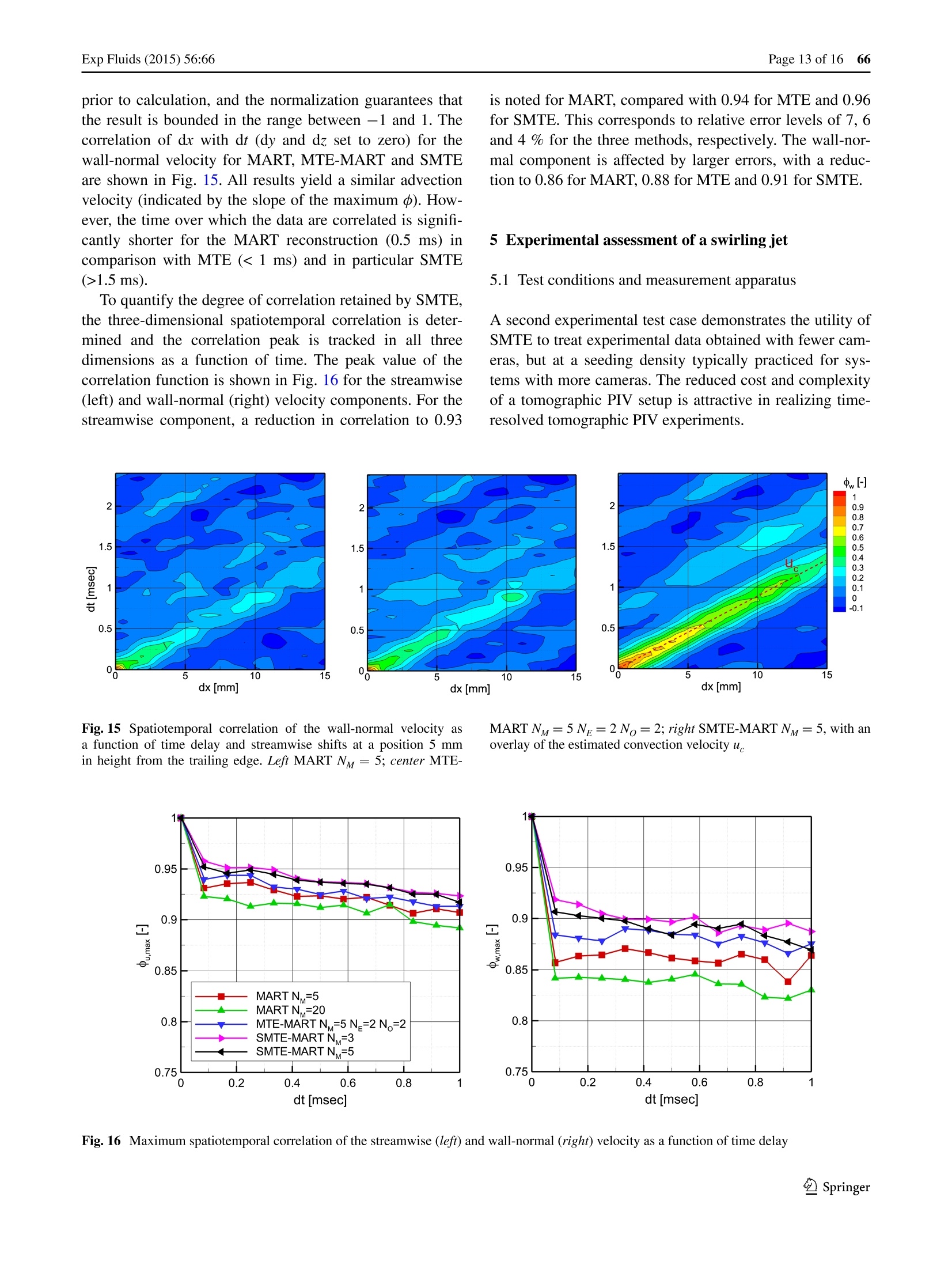
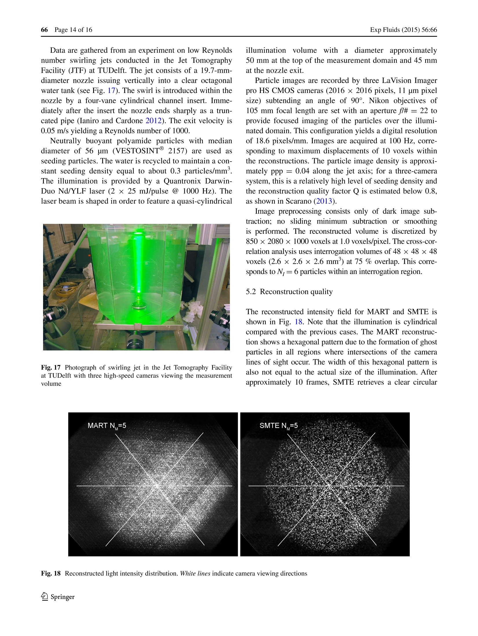
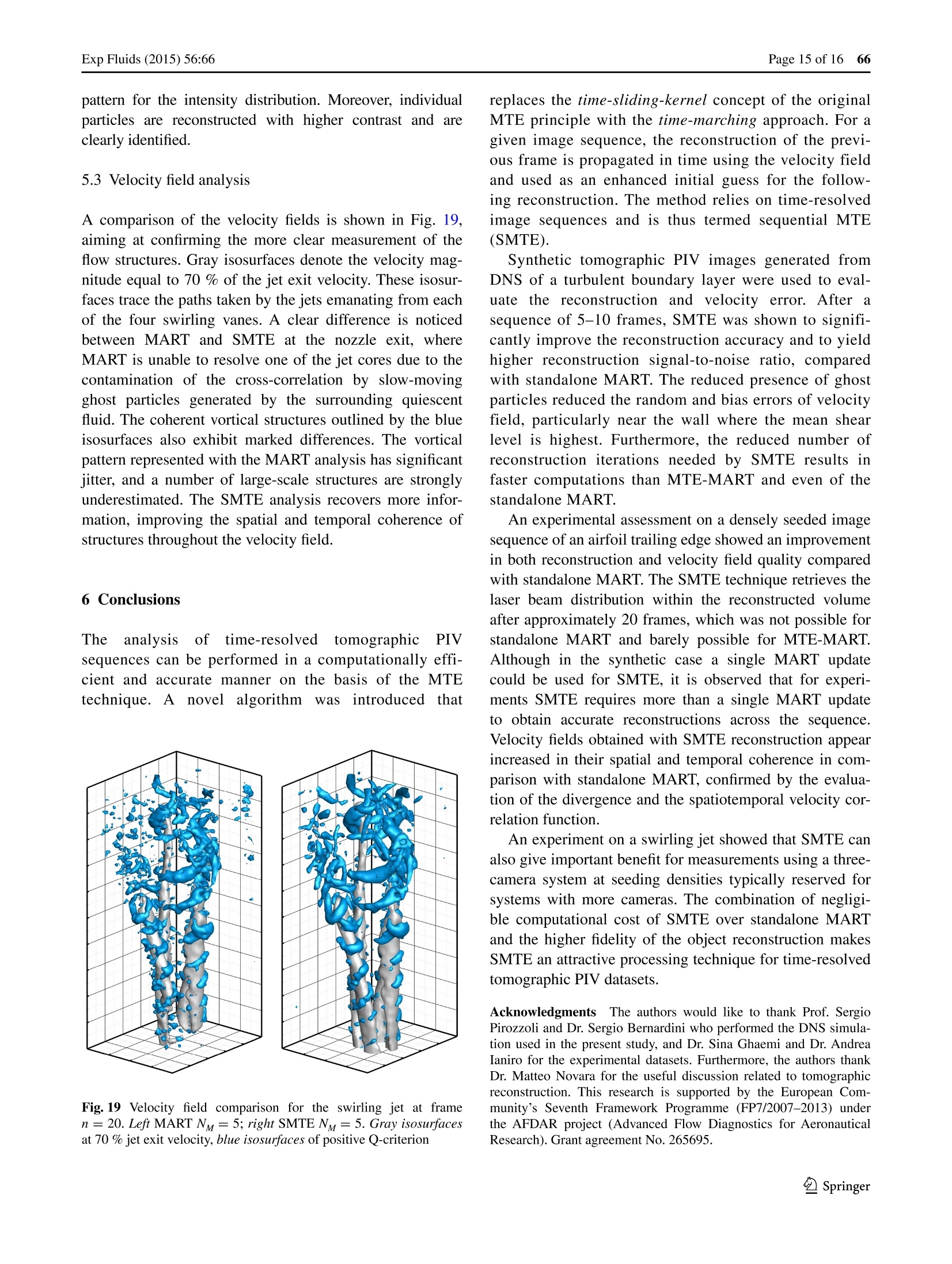
Exp Fluids (2015) 56:66DOI 10.1007/s00348-015-1934-6 66 Page 2 of 16Exp Fluids (2015) 56:66 An efficient and accurate approach to MTE-MARTfor time-resolved tomographic PIV K. P. Lynch·F. Scarano Received: 22 September 2014/ Revised: 18 January 2015 / Accepted: 26 February 2015/ Published online: 13 March 2015O The Author(s) 2015. This article is published with open access at Springerlink.com AbstracttThe motion-tracking-enhanced MART (MTE-MART; Novara et al. in Meas Sci Technol 21:035401,2010) has demonstrated the potential to increase the accu-racy of tomographic PIV by the combined use of a shortsequence of non-simultaneous recordings. A clear bottle-neck of the MTE-MART technique has been its compu-tational cost. For large datasets comprising time-resolvedsequences, MTE-MART becomes unaffordable and hasbeen barely applied even for the analysis of densely seededtomographic PIV datasets. A novel implementation isproposed for tomographic PIV image sequences, whichstrongly reduces the computational burden of MTE-MART,possibly below that of regular MART. The method is asequential algorithm that produces a time-marching esti-mation of the object intensity field based on an enhancedguess, which is built upon the object reconstructed at theprevious time instant. As the method becomes effectiveafter a number of snapshots (typically 5-10), the sequen-tial MTE-MART (SMTE) is most suited for time-resolvedsequences. The computational cost reduction due to SMTEsimply stems from the fewer MART iterations requiredfor each time instant. Moreover, the method yields supe-rior reconstruction quality and higher velocity field meas-urement precision when compared with both MART andMTE-MART. The working principle is assessed in termsof computational effort, reconstruction quality and veloc-ity field accuracy with both synthetic time-resolved tomo-graphic images of a turbulent boundary layer and twoexperimental databases documented in the literature.Thefirst is the time-resolved data of flow past an airfoil trailing ( K. P. Lynch (区)· F. Scarano ) ( e-mail: k.p.lynch@tudelft.nl ) edge used in the study of Novara and Scarano (Exp Fluids52:1027-1041,2012); the second is a swirling jet in a waterflow. In both cases, the effective elimination of ghost parti-cles is demonstrated in number and intensity within a shorttemporal transient of 5-10 frames, depending on the seed-ing density. The increased value of the velocity space-timecorrelation coefficient demonstrates the increased velocityfield accuracy of SMTE compared with MART. 1 Introduction Time-resolved tomographic PIV isis a specific measure-ment regime of the tomographic PIV technique (Elsingaet al. 2006) characterized by a high degree of spatial andtemporal coherence between subsequent measurements. Inpractice, this is realized using high-speed camera and lasersystems to acquire image sequences typically composedby hundreds or thousands of recordings. When the systemoperates in sequential mode, the images are recorded at atime separation that is small enough to enable their cross-correlation. As a result, the spatial and temporal develop-ment of a flow is vividly captured. The breadth of informa-tion contained in these sequences has led to its applicationto investigate unsteady flow phenomena (see, e.g., the panelof applications in the review of Scarano 2013). Among themost prominent applications of time-resolved tomographicPIV are the unsteady pressure evaluation (van Oudheusden2013), aeroacoustic estimation (Violato and Scarano 2013;Probsting et al. 2013)and the study of fundamental mecha-nisms in turbulent shear flows (Elsinga and Marusic 2010;Schroeder et al. 2011). A constraining factor in all tomographic PIV experi-ments is the measurement error introduced by reconstruc-tion. The error has multiple sources: imaging artifacts (e.g., out-of-focus blur, Schanz et al. 2013a), calibrationinaccuracies (Wieneke 2008), background reflections andcamera noise; however, the predominant source is due toghost particles (Elsinga et al. 2006). At a low-to-moderatelevel of particle image density (e.g., for a system of fourcameras and particles per pixel, ppp < 0.05), the peakintensity of ghost particles is significantly lower than thatof actual particles and their effect on cross-correlation canbe neglected. However, experiments requiring high spatialresolution involve a greater particle concentration, leadingto increased particle image density (i.e., ppp>0.1). In thisregime, ghost and actual particles share similar peak inten-sity, with significant detrimental effect on the cross-correla-tion (Elsinga et a. 2011). This limitation has motivated multiple efforts to reducethe number and intensity of ghost particles in the recon-struction. The spatial filtering improved reconstruction(SFIT) approach by Discetti et al. (2013) uses a tailoredfiltering of the reconstructed volume between reconstruc-tion iterations to regularize reconstructed particle shapesand partly filter out ghost particles. The simulacrum match-ing-based reconstruction enhancement (SMRE) techniqueproposed by de Silva et al. (2013) removes ghost particlesa posteriori of the reconstruction process based on somehypotheses on the shape of the particles. Another a poste-riori approach by Elsinga and Tokgoz (2014) is based onparticle tracking velocimetry (PTV). With a long sequenceof time-resolved images, ghost particles could be unambig-uously identified and removed. A substantial reduction in ghost particles has beenachieved using methods that exploit the coherence of par-ticles over two or more frames within the reconstruction.The first method in this category is the motion-tracking-enhanced MART (MTE-MART; Novara et al. 2010). Theworking principle is the combined use of recordings takennon-simultaneously to produce an enhanced first guess forthe tomographic reconstruction algorithm. The methodfeatures an iterative procedure of reconstruction and cross-correlation whereby the velocity field is used to deformthe reconstructed object and obtain an enhanced initialguess for the reconstruction at a different time instant. Itsapplication to turbulent shear flows (Novara and Scarano2012) showed that a seeding density up to 0.2 ppp couldbe afforded by a four-camera system. It was concludedthat MTE-MART makes a significant improvement withrespect to regular MART when a kernel of 3-5 exposuresis considered. However, in the latter conditions, the compu-tational effort becomes more than one order of magnitudegreater than the standard method, based on MART recon-struction followed by cross-correlation analysis. This is dueto the iterative approach applied to the whole time kernel toobtain the reconstruction at a given time instant. Efficientreconstruction procedures such as MLOS-SMART have been proven compatible with the MTE principle and allevi-ate the computational burden (Atkinson et al. 2010). How-ever, for time-resolved tomographic PIV, where thousandsofimages are involved, the additional computational costof all MTE methods has so far precluded its widespreaduse, possibly resulting in a stagnation of developments onthis topic. The second method in this category is the recentlyintroduced ‘shake-the-box'(STB) method of Schanz et al.(2013b), which combines 3-D PTV with the iterative parti-cle reconstruction (IPR) method of Wieneke (2013). Parti-cles are tracked in 3-D space over multiple frames provid-ing a Lagrangian description of the fluid motion and cleardiscrimination criteria for the elimination of ghost particlesfrom reconstructions. Furthermore, the method is compu-tationally efficient in comparison with the voxel-basedreconstruction procedures. The STB method has been firstapplied to water flows using a tomographic system com-posed of six high-speed cameras. A recent numerical eval-uation of the method (Schanz et al. 2014) has shown theability of STB to strongly remove ghost particle intensityfor time-resolved sequences. The present article recognizes the principle of motiontracking in image sequences for enhancing the tomographicreconstruction and proposes a novel implementation ofMTE-MART that exploits the potential of this concept interms of both computational efficiency and attainable accu-racy. The working principle is first elucidated, followed bya detailed assessment based upon a synthetic time-resolvedtomographic PIV experiment of a turbulent boundarylayer with data produced from a direct numerical simula-tion (Probsting et al. 2013). The experimental verificationmakes use of the time-resolved image sequence proposedby Novara et al. (2012) regarding the turbulent wake behindthe trailing edge of an airfoil. A second experiment of aswirling jet illustrates the potential of SMTE for accuratereconstruction using a three-camera tomographic system. 2 SMTE working principle The primary concept of MTE-MART (Novara et al. 2010)is that subsequent exposures contain essentially the sameparticle field. Such information can be used in the recon-struction of a single snapshot. Because the particles appearwith slightly different (relative) position along the expo-sures, the reconstruction can be improved by reducing theambiguity of the MART solutions if all these views can beused to generate an a priori condition for the first guess ofthe MART calculation. However, for the improved recon-struction of a single snapshot, MTE makes use of a finitetemporal kernel, where knowledge of the reconstructedintensity field and the velocity field at all time instants is required. This is achieved with an iterative procedure.For time-resolved measurements, this operation can beregarded as a time-sliding-kernel approach for MTE evalu-ation. In the first iteration, the initial guess of voxel inten-sity for the reconstruction is set as uniform (typically unit)value. Following the discussion and the nomenclatureintroduced by Novara and Scarano (2012), the numberof enhancement iterations Ng is the primary driver of thecomputational cost, with typical increases of 3-10 timesfor analysis of an image pair (No=2). Extending the sizeof the temporal kernel (effectively, the number of objectsN) to three or five does yield an improved accuracy, butthe computational cost increases even more rapidly. Anadditional bottleneck preventing the use of large kernelsis the less accurate prediction of particles motion, possiblyaffected by truncation errors. The main variation introduced in the present workto the MTE method is changing the time-sliding-kernelapproach into a time-marching algorithm. The latter can beapplied to image sequences as typically acquired in time-resolved tomographic PIV experiments. Once the velocityfield associated to the first two snapshots is estimated, anenhanced initial guess for the reconstruction of the thirdsnapshot EG,3 can be obtained by propagating the previousreconstruction E, forward in time via the velocity field. Fora generic frame number n, the relation reads as: where the vector R=(X,Y,Z) indicates object space coor-dinates. The propagation is identical to that followed for theimage deformation methods (Huang et al. 1993; Scarano2002) and is applied as three-dimensional (volume) defor-mation in this case. The sequential approach justifies theterm sequential motion-tracking-enhanced MART (SMTE-MART). A schematic description of the procedure is givenby the following steps and graphically illustrated with theflow chart of Fig. 1. It is assumed that the sequence startswith frame number n = 1: I. O(bject reconstruction If n=1: reconstruct pair E and E If n>1: reconstruct En+1, using initial guess E+ 2. Velocity field calculation (a)Cross-correlation of the pair En@ En+1 yieldsvelocity Vn 3. Enhanced guess estimation for the subsequent snapshot Estimate velocity V'n+1 (see Eq.2) Build enhanced guess E2 by deforming En+1 byV'n+1 (see Eq. 1) Fig. 1 Schematic flow chart of SMTE-MART. I indicates the set ofcamera images at frame n. Dashed boxes include the images and thefirst guess intensity field used for MART 4 Time marching (a))Increment n and return to step (1b) The velocity at the upcoming frame Vn+1 is estimatedas Vh+i making use of a time forward approximation in theassumption of advection. This approach is valid when thetime separation between frames At is small relative to theflow time scales, which generally applies for time-resolvedPIV sequences. The advection assumption was shown to yield a goodapproximation of the velocity temporal evolution whenthe two components of the material acceleration dV/dtand V.VV are equal and opposite, yielding DV/Dt ≈0.Under this condition, known as frozen turbulence, whichoccurs in turbulent flows with moderate levels of shear, theabove equation was proven accurate for the prediction ofthe velocity in between measured time instants (time super-sampling, Scarano and Moore 2012). A more generallyvalid time-prediction methods (e.g., vortex-in-cell, Sch-neiders et al. 2014) may be considered for more complexflows (e.g., the separated region of wakes and free shearlayers in jets) and when the time separation between framesis enlarged. Two practical notes on the numerical implementationof the method should be mentioned. First, extrapolationof the object intensity in the generation of the enhancedguess should be given a nonzero value to allow the buildupby multiplicative update of the intensity along inflow boundaries of the reconstructed domain. A practical choiceproposed herein is that voxels at the volume boundary areset to a value corresponding to the mean intensity of thereconstructed volume. Second, the two snapshots at thebeginning of the sequence E and E, shall be reconstructedwith the standard MART algorithm with the typical numberof iterations (NM=5). This enables a faster convergence ofthe results along the sequence. The number of MART itera-tions for the following snapshots can be reduced to three oreven less, as discussed in the remainder of the article. A number of advantages are expected when the MTEprinciple is applied in time-marching mode along thesequence. First, the accuracy of the enhanced guess willimprove throughout the sequence and increase its sparsityas the space where no particles are present is progressivelydetermined. This condition enables to reduce the number ofMART iterations needed for the convergence of a snapshotreconstruction. Second, as the effective number of exposuresNo increases along the sequence, the effect of virtually mul-tiplying the number of viewing cameras is exploited, eventu-ally surpassing that typically achieved by MTE-MART. The performance of the SMTE-MART algorithm fol-lows that of MTE-MART in terms of ghost intensity sup-pression and enhancement of actual particles reconstruc-tion. Also the increase in correlation signal-to-noise ratio,as discussed in Novara et al. (2010) and Novara andScarano (2012), is retrieved back in the current study. A topic of particular concern for time-marching algo-rithms is stability: For MTE-MART, it was demonstratedthat the worst-case performance (e.g., due to an erroneousvelocity vector field) corresponds to the standard MARTsolution due to the multiplicative nature of the MARTupdate, which prevents an incorrect enhanced guess fromdegrading the final solution (Novara et al. 2010). The sameprinciple applies to SMTE-MART, which therefore in theworst-case scenario corresponds to standard MART with anequal number of reconstruction iterations. As a final note, the general nature of the sequentialalgorithm makes it suited to other iterative reconstructionalgorithms such as MLOS-SMART (Atkinson and Soria2009) or BIMART (Thomas et al. 2014), where furtherimprovements may be obtained in terms of computationalefficiency. Since the MART algorithm is the most widelyreferred to in the literature, the present study uses it forreconstruction. 3 Assessment from simulated turbulent boundary layer 3.1 Test case and data processing The performance of SMTE-MART is first investigated inabsence of calibration errors and imaging noise. Synthetic tomographic PIV images ofa turbulent boundary layer overa flat plate are generated following a direct numerical simu-lation (DNS) from Bernardini and Pirozzoli (2011). Detailsof the simulation and data discretization are given in thework of Probsting et al. (2013) who verified the suitabilityof tomographic PIV for determining the spectral coherenceof surface pressure fluctuations. 1Theesimulated1measurementldomainencompasses21.6x10.8×10.8 mm’ along streamwise (X), spanwise(Y) and wall-normal (Z) directions, respectively.The thick-ness of the turbulent boundary layer is 89g = 12 mm, andthe associated Reynolds number is Re~ 8185. The par-ticle concentration is set to 25 part/mm’, yielding a parti-cle image density of 0.2 ppp. Particles are randomly dis-tributed in space, and their motion is calculated from theDNS velocity fields using a fourth-order Runge-KuttaODE solver. A thin buffer region on all boundaries is usedto allow particles entering and leaving the simulated meas-urement domain. The particle blobs are generated using 3-D Gaussianintegration onto a voxel grid (adapted from Lecordier andWesterweel 2004). Camera images are obtained by project-ing the 3-D particle positions onto 2-D sensors via a pin-hole camera model (Tsai 1987) and performing 2-D Gauss-ian integration onto a pixel grid. The size of the projectionimages is 1050 × 600 px, with a particle image diameterof approximately 2.5 px. The simulation employs fourcameras with viewing directions of 30° from the normal tothe wall along both directions (cross-configuration), cor-responding to a system aperture of 60° along horizontaland vertical direction, a commonly adopted and favorableconfiguration for tomographic imaging and reconstruction(Scarano 2013). The tomographic reconstruction with MART followsthe numerical recipe given by Elsinga et al. (2006). Thenumber of MART iterations NM is varied in the analysis; aGaussian smoothing of the object is applied between suc-cessive MART iterations on a kernel of 3 x 3× 3 voxels.The reconstructed volume size is 964 x 532 × 532 voxelswith a non-illuminated buffer of 50 voxels on each bound-ary that prevents edge effects in the reconstruction andallows calculating the reconstruction signal-to-noise ratio.The chosen discretization is based upon a voxel/pixel ratioof 1.0, resulting in a resolution of 40 vox/mm. detection (Westerweel and Scarano 2005) and replacedwith a distance-weighted neighborhood average. No spa-tial filtering/smoothing is applied to the final vector field. Atime-marching predictor of the cross-correlation is used tobypass the need for multi-grid evaluation and accelerate theprocessing, as used by, e.g., Scarano and Poelma (2009). 3.2 Reconstruction quality Several metrics are invoked to evaluate the accuracy ofthe reconstructed objects. First, the reconstructed lasersheet intensity distribution is visualized along a plane thatincludes the depth direction. Regions of the reconstructionwithin the laser sheet contain both real and ghost particles,while regions outside the laser sheet contain only ghostparticles (a top-hat laser beam model was applied for theillumination). A well-accepted verification criterion for thetomographic reconstruction is the ability to clearly identifythe laser sheet within the reconstructed volume (Scarano2013). A central principle of the MTE-MART technique isthe reduction in ghost particles intensity and the increasein real particles intensity (Novara et al. 2010). In Fig. 2(right), the diagrams indicate a ratio of intensity of approxi-mately 2.5:1 for the MART reconstruction with 5 iterationsand 3.3:1 when the number of iterations is increased to 20.MTE-MART returns an intensity distribution comparableto the latter case. The application of SMTE-MART leads inpractice to the elimination of ghost particle intensity. Inter-estingly, the same result seems to be obtained, irrespec-tive of the number of MART iterations adopted for eachsnapshot. The reconstruction signal-to-noise ratio, SNR isdefined as the ratio of mean intensity inside the and outside the illuminated region. A minimum value of 2 is considereda criterion for an acceptable reconstruction (Scarano 2013).Clearly, greater values of SNR correspond to a reducedcontribution from ghost particles. The SNRe is shown inFig. 3.MART reconstructions with 5 or 20 iterations returnvalues of 2.0 and 3.3, respectively. The increase in SNRwith additional MART iterations is a behavior typicallyencountered using synthetic data where image noise is notconsidered. In experimental data instead (see Sect.4), theimprovement of reconstruction quality Q after 5 MARTiterations becomes less pronounced. SMTE-MART beginswith a reconstruction SNR equal to the MART case andincreases rapidly (one order of magnitude after 5 frames)reaching a converged value (independent of further timeadvancement) of approximately 100 after approximately15 frames. This result also seems to be independent ofNM, although the rate of convergence increases slightlywith NM.Remarkably, for all considered values of NM, theSNRe obtained after convergence is significantly higherthan MART Nw=20. This indicates that the reconstruc-tion accuracy of SMTE-MART is not only related to thelarger number of MART iterations (considered along thesequence), but mainly due to the fundamental principleof MTE, whereby the particles with coherent motion areretained along several frames against the incoherent ghostparticles. A second evaluation criterion is the reconstructionquality factor Q as originally proposed by Elsinga et al.(2006), defined as the normalized cross-correlation coef-ficient between the reconstructed and exact object. Com-pared with the SNRe, which is predominantly an esti-mate of ghost formation, Q also yields a measure of thespatial accuracy in the reconstruction of actual particles. For example any small positional inaccuracy due to inac-curate correction lby SMTE-MART of the incomingenhanced guess would result in considerable decrease inQ. The results shown in Fig. 3 indicate that the above circumstance is not encountered, at least for the present case.The comparison yields Q=0.87 (at all values of Ny) forSMTE, whereas the highest value obtained with MART atNy=20 is Q=0.67, MTE-MART returns a value slightlyexceeding 0.7. The analysis of ghost particles reduction is performedby direct inspection of occurrence and peak intensity ofghost particles within the volume. Reducing the presenceof ghost particles is reported to yield an improved cross-correlation analysis as their presence potentially corruptsthe cross-correlation map in proximity of the peak, result-ing in a bias toward lower values of the velocity gradient(Elsinga et al.2010). The number of frames required for SMTE to reachconvergence may raise issues on its application to shortsequences (e.g., high-speed burst systems). However, asfor any sequential algorithm, SMTE can also be appliedbackward in time after marching along the sequence inthe forward direction. The resulting ‘forward-backward'SMTE will become more computationally expensive, butstill yield a benefit compared with standard MART or MTEin short sequences (typically 2-8 frames). For brevity, thismode of operation is not discussed further. The particle detection scheme required for this analysisassumes a 3-D Gaussian blob for the real particles. Any par-ticle found within one voxel distance from the position of areal particle is considered a valid match. All other peaks areassociated to ghost particles. A histogram of the real andghost particle intensities for MART and SMTE is givenin Fig. 4 for frame n =20. The vertical axis is truncatedto clearly illustrate the distribution of real particles. TheMART reconstruction yields an intensity of real particlesthat largely overlaps with that of the ghost particles. In con-trast, SMTE establishes a clear range separation between Fig.3 Left reconstruction signal-to-noise ratio SNRp. Right reconstruction quality factor Q Fig. 4 Histogram of peak intensities for MART (left) and SMTE (right). Ghost particles in red, real particles in black. Vertical axis truncated toease visualizing the intensity distribution of real particles peak intensity of real and ghost particles. This behavior isconsistent with previous reports on MTE-MART (Novaraet al.2010). A similar behavior is noted in the number of ghost/realparticles. The ratio of generated ghost particles to real onesis approximately 25 for MART and drops to 5 for SMTE.In both cases, the number of real particles generated isnearly equal to the actual simulated particles. 3.3 Velocity field analysis The velocity field accuracy is first assessed qualitatively byvisual inspection of its spatial coherence in comparison withthe velocity field obtained by cross-correlation analysis ofthe exact particle field. Furthermore, the quantitative analy-sis is based on the absolute error level. A visual comparisonof the velocity field at frame number n= 20 is shown inFig. 5. The reference case is chosen as the cross-correlation of the exact intensity field in order to account only for theerrors due to the reconstruction and not those associatedwith the finite spatial resolution. The objects reconstructedwith MART (NM=5) and SMTE-MART (NM=3) are con-sidered. Contours of the streamwise velocity along a planeparallel to the wall and isosurfaces of positive values of theQ-criterion for visualization of vortical structures are repre-sented. The reference velocity field features regions of highand low velocity. Around the latter, vortical structures aremore often detected,elongated along the streamwise direc-tion or under form of arcs and canes. A hairpin like structureis visualized in the top-right region of the selected field, atopan elongated low-speed region. This is consistent with theobserved pattern of coherent structures in turbulent bound-ary layers at the current Reynolds number (Adrian 2007). An inspection of the result obtained with the MART recon-struction yields isosurfaces with no evidence of the charac-teristic vortical structures. Moreover, the streamwise velocity contours, which in the reference field reveal elongated alter-nating streaks of high- and low-speed fluid near the wall,are less distinct with the MART reconstruction and appeargenerally biased toward higher velocity values. The latter isascribed to high velocity outlier vectors due to ghost particlesgenerated by particles in the outer layer and forming closerto the wall. The tracer particles traveling at approximatelyfreestream velocity form the largest number of ghost particlesalong the entire depth of the measurement domain. Thus, thecorrelation near the wall with MART is heavily biased by alarge number of fast-moving ghost particles, which dominatethe signal against a smaller number of slowly moving actualparticles subject to strongly sheared motion. Many of the features observed in the reference veloc-ity field can be retrieved in the analysis conducted with theobjects reconstructed with SMTE. Although a higher noiselevel is observed, the scenario is considerably more favora-ble within the SMTE results, with the alternating streaksclearly identified in agreement with the reference field. The measurement accuracy is assessed quantitatively byevaluation of the total error, determined by the RMS of thedifference between the measured and actual velocity field.In Eq. 3, i is the grid node index and N the total number ofvectors in the measurement domain. The total error, varying along the sequence of frames,is reported in Fig. 6. In this case, the reference velocityfield is given by the DNS data. The data series showing thesmallest error (approximately 0.1 voxels) is that obtainedcross-correlating the exact particle field. The level of theerror associated to the analysis with 5 MART iterations is Fig. 6 Total RMS error. Reference curve indicates correlation per-formed on reference objects (no reconstruction errors) above 0.6 voxels, which compares well with a recent studyof tomographic PIV measurement uncertainty from theauthors (Lynch and Scarano 2014). Increasing the num-ber of iterations to 20, the minimum error level achievableusing MART is approximately 0.4 voxels. Based on thefreestream displacement of 12 voxels, the correspondingdynamic velocity range (DVR; Adrian 1997) of this simu-lated measurement reduces to only 30 levels. The SMTEresult converges to a total error between 0.15 and 0.2 vox-els, depending on the number of MART iterations. Theclose approximation to the result obtained cross-correlatingthe reference objects indicates that SMTE has reduced theoccurrence of ghost particles to a level that is negligible. 3.4 Computational time The computational effort required to realize MTE-MARTwas already reported as being much greater than standardMART processing (Novara et al. 2010). Given that MARTcalculations are already computationally demanding, theapplication of MTE-MART has become impractical for largeimage sequences. In contrast, the SMTE-MART proceduredoes not require additional iterations and achieves a supe-rior result to both standalone MART and MTE even whenfewer MART iterations are used. The only additional com-putational step over MART is the generation of the enhancedguess. The computational cost is summarized in Fig. 7,where the approximate wall-clock time required for each ofthe processing tasks is shown. The computation time is bro-ken into segments for reconstruction, correlation and (in thecase of MTE and SMTE) enhanced guess generation. The result is averaged over the 25 frames considered, not includ-ing the initial reconstructions performed using 5 MART iter-ations. The wall-clock time is approximated by dividing theCPU time by the number of CPU cores (presently 48). Both the SMTE Ny=1 and Ny=3 results have a com-putation time shorter than even the standalone MART, atunder 10 min per frame. Furthermore, the computationalload of cross-correlation exceeds that of the reconstruction.In contrast, the case of MART Ny=20 takes four times aslong to reconstruct as the MART NM=5 case, but with anidentical time spent in cross-correlation. Finally, the MTEis longer in both reconstruction and cross-correlation due tothe iterative procedure. In total, the SMTE approach resultsin a method over four times faster than MTE and margin-ally less time consuming when compared to MART. 4 Experimental assessment of a turbulent trailing edge 4.1 Test conditions and measurement apparatus The present analysis follows closely that performed byNovara and Scarano (2012). Data are gathered from a time-resolved tomographic PIV experiment on turbulent flowpast the trailing edge of an airfoil. Details of the experi-ment are provided in Ghaemi and Scarano (2011) The airfoil model is a NACA-0012 of 40 cm chordplaced at zero angle of attack. The freestream velocity is14 m/s, yielding a chord Reynolds number of 370,000. Theboundary layer thickness 8gg at the trailing edge is 9.5 mm.At this location a measurement volume of 40 × 24×8 mmis realized. The experimental apparatus consists of aQuantronix Darwin-Duo Nd:YLF laser (2×25 mJ/pulse at 1 kHz) and four high-speed Photron Fastcam SAI CMOScameras (1024 × 1024 pixels at 5400 fps). The illumina-tion is increased by the multi-pass technique,reflecting thebeam multiple times throughout the volume (Ghaemi andScarano 2010). Seeding is provided by a stage smoke gen-erator producing particles with 1 um nominal diameter. The cameras are fitted with 105 mm focal length Nikonobjectives operating at f/# = 22 and arranged in a linearconfiguration (see Fig.8). The particle image diameter d, is1.5 px as determined via autocorrelation analysis. Both thelaser and camera systems are operated in single-frame con-tinuous mode to record a time-resolved image sequence ata frequency of 12 kHz. Synchronization and image acqui-sition are controlled from a PC with LaVision DaVis 7.4software and a high-speed controller. Two experiments are conducted at a particle image den-sity of 0.05 and 0.2 ppp. These correspond to particle con-centrations of 3 and 12 particles/mm’, respectively. Detailson the particle density estimation can be found in Novaraand Scarano (2012). Image preprocessing consists of twosteps: First, the historical minimum is calculated at eachpixel for each camera. Then, the images are subtractedby the corresponding minimum. The images are furtherdivided by the time-average value at each pixel to normal-ize the intensity within each camera image and amongcameras. No spatial filtering (smoothing) is applied. Exam-ple preprocessed images are given in Fig. 8. The case ppp = 0.05 is used to refine the camera map-ping functions via the volume self-calibration technique(Wieneke 2008). Residual calibration errors are below0.1 pixels. The reconstructed volume is discretized by900×550×250 voxels with a pixel-to-voxel ratio of 1.0.The cross-correlation analysis is identical to the synthetic Fig. 8 Left tomographic PIV setup (reproduced from Ghaemi and Scarano 2011). Right individual particle images after preprocessing (cropped.to 500×200 pixels) at ppp=0.05 (top) and 0.2 (bottom) case, but using interrogation volumes of 24 × 24 ×24voxels (1.2× 1.2×1.2 mm’) at 75 % overlap. This cor-responds to N=15 particles within an interrogation regionfor ppp=0.2. 4.2 Reconstruction quality The laser sheet intensity distribution for the reconstructedvolume of frame 35 in the sequence is given in Fig. 9. TheMART (NM =5) reconstruction has an intensity distribu-tion that does not exhibit any region with higher inten-sity. Therefore, also the edges of the illuminated regionare not visible. Increasing iterations (NM =20) and usingthe MTE-MART deliver a small region of local maximumbarely distinguishable above the background level. Withthe introduction of SMTE-MART the boundaries of theilluminated volume become better defined. Note that theSMTE-MART NM = 1 (a single MART update), althoughbetter than regular MART and MTE-MART, is less definedthan the cases with additional MART updates. The SNR is calculated by considering an average ofregions inside and outside of the illuminated volume andis displayed in Fig. 10. The trend is similar to that observedearlier in the synthetic data (see Fig. 3): The SNR ofMART remains below 1.2 and MTE yields a value approxi-mately 1.5. The SNR of SMTE-MART increases alongthe sequence, requiring 15-30 frames to approach a valueof 3. The SMTE results with a single MART iteration arepoorer (SNR <2) than those obtained with 3 or 5 itera-tions, confirming the previous observation and indicatingthat for experimental data, there is benefit in using morethan a single MART update with SMTE-MART. Fig. 10 Reconstruction signal-to-noise ratio, SNRp. Legend identicalto Fig. 9 4.3 Velocity field analysis A rendering of the instantaneous velocity field is shown inFig. 11. The blue isosurfaces represent low-speed regions(50 % of the freestream velocity) throughout the velocityfield. Brown isosurfaces indicate positive values of Q-cri-terion. A significant difference in the low-speed streaks isseen between MART and SMTE, the former being unableto capture the streaks throughout the entire streamwisedirection. Furthermore, an improvement in the spatialcoherence of the Q-criterion is evident in the SMTE result,which allows a less ambiguous identification of hairpin andcane structures. x/8gg-] Fig. 11 Instantaneous velocity field snapshot for frame n = 30 using MART (left) and SMTE Ny =5 (right).Blue isosurfaces are streamwisevelocity 50 % of the freestream velocity, and brown isosurfaces are of positive Q-criterion Fig. 12 Overview of coherent structures identified by the Q-criterion for MART N =5 (left) and SMTE Ny=5 (right). Regions A and B des-ignate two convecting hairpin structures Time-resolved tomographic PIV has been recentlyused to investigate the temporal evolution of coherentstructures (Schroder et al. 2011; Elsinga et al.2012). Theprediction of properties such as the lifetime of energy-containing eddies (Elsinga and Marusic 2010) and theirstability strongly relies on an accurate description oftheir spatial pattern and their temporal evolution and themeasurement noise plays a crucial role in biasing theestimate of such properties. The comparison of MARTand SMTE is given here through visualization of thesestructures at subsequent recordings. In Fig. 12, a portionof the data is shown for four time instants where isosur-faces of Q-criterion are used to identify hairpin and canestructures. The isosurfaces are color-coded blue to red todesignate subsequent time instants. A higher spatial andtemporal coherence is observed for the results obtainedwith SMTE reconstruction. In contrast, the results based on the MART reconstruction are much more difficult tointerpret in terms of time sequence. A more objective assessment of the measurement pre-cision is made invoking the assumption of incompress-ible flow whereby the velocity field divergence is zero.A nonzero measured value gives an estimate of the errorin determining the tensor (Zhang et al. 1997) and furtherderived quantities such as the Q-criterion. A PDF of thedivergence is given in Fig. 13 (left). Compared with MART,the SMTE exhibits a narrower distribution around zero,indicating a measurement better satisfying this condition.The performance of all methods throughout the sequence isassociated to the standard deviation of the divergence andillustrated in Fig. 13 (right). Beginning from a nearly equalvalue at the start of the sequence, the SMTE decreasesover approximately 10 frames to a value about 1.5 timesless than MART (i.e., approximately 0.07 vox/vox from Fig. 14 PDF of the correlation signal-to-noise ratio (SNR) for framen=30. Legend identical to Fig.9 0.11 vox/vox). The decrease in divergence for the first 1-2frames of normal MART cases is due to the time-marchingpredictor for the cross-correlation as mentioned earlier. Finally, the robustness of the measurements is inquiredusing the cross-correlation signal-to-noise ratio (SNR),defined by the ratio of highest to second highest peak inthe 3-D correlation map. A value >1.5 is often consideredas acceptance criterion for a reliable correlation analysis(Keane and Adrian 1990). In Fig. 14, the PDF of SNR isshown for MART and SMTE. The former has a distribu-tion with maximum occurrence in the range between 1.2and 1.5. MTE is slightly shifted to higher values with aplateau up to a value of 2. The SMTE analysis is centeredaround a value of 3.5. The slight shift of the distributionswith varying number of MART iterations in SMTE maynot be regarded as an improvement in the measurement robustness. It is instead ascribed to the residual of the inten-sity field transported from the previous recording. Assuming that velocity fluctuations are passively trans-ported by the flow, the measurement precision can be esti-mated a posteriori making use of the space-time correlationfunction. The time that separates uncorrelated measure-ments is their temporal separation △t = 83 us. Novaraand Scarano (2012) provided an estimate of the Lagran-gian time scale for the intrinsic evolution of turbulent fluc-tuations, which was estimated in the order of 10 ms: twoorders of magnitude longer than At. As a consequence, ahigh degree of correlation is expected between the velocityfields in a time series of 10-30 frames. Any rapid drop ofthe velocity spatiotemporal correlation peak from the unitvalue at the origin signals the presence of noisy fluctuationsaffecting the measurement. The precision is therefore estimated by considering thedrop of the maximum value of the spatiotemporal correla-tion function. A similar approach was followed by Sciac-chitano et al. (2012) and Lynch and Scarano (2013). Thespatiotemporal correlation function of the streamwisevelocity component between two subsequent exposuresseparated by a time delay dt and displacements dx, dy anddz is 中u(dx,dy,dz,dt) (4) where N is the number of grid nodes in the measurementdomain. The mean value of the velocity field is subtracted prior to calculation, and the normalization guarantees thatthe result is bounded in the range between -1 and 1. Thecorrelation of dx with dt (dy and dz set to zero) for thewall-normal velocity for MART, MTE-MART and SMTEare shown in Fig. 15. All results yield a similar advectionvelocity (indicated by the slope of the maximum (). How-ever, the time over which the data are correlated is signifi-cantly shorter for the MART reconstruction (0.5 ms) incomparison with MTE (<1 ms) and in particular SMTE(>1.5 ms). To quantify the degree of correlation retained by SMTE,the three-dimensional spatiotemporal correlation is deter-mined and the correlation peak is tracked in all threedimensions as a function of time. The peak value of thecorrelation function is shown in Fig. 16 for the streamwise(left) and wall-normal (right) velocity components. For thestreamwise component, a reduction in correlation to 0.93 is noted for MART, compared with 0.94 for MTE and 0.96for SMTE. This corresponds to relative error levels of 7, 6and 4 % for the three methods, respectively. The wall-nor-mal component is affected by larger errors, with a reduc-tion to 0.86 for MART, 0.88 for MTE and 0.91 for SMTE. 5 Experimental assessment of a swirling jet 5.1 Test conditions and measurement apparatus A second experimental test case demonstrates the utility ofSMTE to treat experimental data obtained with fewer cam-eras, but at a seeding density typically practiced for sys-tems with more cameras. The reduced cost and complexityof a tomographic PIV setup is attractive in realizing time-resolved tomographic PIV experiments. 2 1.5 1叮M0 0.5 0 15 dx [mm] dx[mm] dx [mm] Fig. 15 Spatiotemporal correlation of the wall-normal velocity asa function of time delay and streamwise shifts at a position 5 mmin height from the trailing edge. Left MART NM = 5; center MTE- MARTNw=5N=2N,=2; right SMTE-MART Nw=5, with anoverlay of the estimated convection velocity u. Fig. 16 Maximum spatiotemporal correlation of the streamwise (left) and wall-normal (right) velocity as a function of time delay Data are gathered from an experiment on low Reynoldsnumber swirling jets conducted in the Jet TomographyFacility (JTF) at TUDelft. The jet consists of a 19.7-mmdiameter nozzle issuing vertically into a clear octagonalwater tank (see Fig. 17). The swirl is introduced within thenozzle by a four-vane cylindrical channel insert. Imme-diately after the insert the nozzle ends sharply as a trun-cated pipe (Ianiro and Cardone 2012). The exit velocity is0.05 m/s yielding a Reynolds number of 1000. Neutrally buoyant polyamide particles with mediandiameter of 56 um (VESTOSINT 2157) are used asseeding particles. The water is recycled to maintain a con-stant seeding density equal to about 0.3 particles/mm’The illumination is provided by a Quantronix Darwin-Duo Nd/YLF laser (2 × 25 mJ/pulse @ 1000 Hz). Thelaser beam is shaped in order to feature a quasi-cylindrical Fig. 17 Photograph of swirling jet in the Jet Tomography Facilityat TUDelft with three high-speed cameras viewing the measurementyolume illumination volumewithadiameter approximately50 mm at the top of the measurement domain and 45 mmat the nozzle exit. Particle images are recorded by three LaVision Imagerpro HS CMOS cameras (2016 ×2016 pixels, 11 um pixelsize) subtending an angle of 90°. Nikon objectives of105 mm focal length are set with an aperture f/#= 22 toprovide focused imaging of the particles over the illumi-nated domain. This configuration yields a digital resolutionof 18.6 pixels/mm. Images are acquired at 100 Hz, corre-sponding to maximum displacements of 10 voxels withinthe reconstructions. The particle image density is approxi-mately ppp = 0.04 along the jet axis; for a three-camerasystem, this is a relatively high level of seeding density andthe reconstruction quality factor Q is estimated below 0.8,as shown in Scarano (2013). Image preprocessing consists only of dark image sub-traction; no sliding minimum subtraction or smoothingis performed. The reconstructed volume is discretized by850×2080×1000 voxels at 1.0 voxels/pixel. The cross-cor-relation analysis uses interrogation volumes of 48 × 48 × 48voxels (2.6×2.6×2.6 mm’) at 75 % overlap. This corre-sponds to N =6 particles within an interrogation region. 5.2 Reconstruction quality The reconstructed intensity field for MART and SMTE isshown in Fig. 18. Note that the illumination is cylindricalcompared with the previous cases. The MART reconstruc-tion shows a hexagonal pattern due to the formation of ghostparticles in all regions where intersections of the cameralines of sight occur. The width of this hexagonal pattern isalso not equal to the actual size of the illumination. Afterapproximately 10 frames, SMTE retrieves a clear circular pattern for the intensity distribution. Moreover, individualparticles are reconstructed with higher contrast and areclearly identified. 5.3 Velocity field analysis A comparison of the velocity fields is shown in Fig. 19,aiming at confirming the more clear measurement of theflow structures. Gray isosurfaces denote the velocity mag-nitude equal to 70 % of the jet exit velocity. These isosur-faces trace the paths taken by the jets emanating from eachof the four swirling vanes. A clear difference is noticedbetween MART and SMTE at the nozzle exit, whereMART is unable to resolve one of the jet cores due to thecontamination of the cross-correlation by slow-movinggrolhost particles generated by the surrounding quiescentfluid. The coherent vortical structures outlined by the blueisosurfaces also exhibit marked differences. The vorticalpattern represented with the MART analysis has significantjitter, and a number of large-scale structures are stronglyunderestimated. The SMTE analysis recovers more infor-mation, improving the spatial and temporal coherence ofstructures throughout the velocity field. 6 Conclusions Theanalysis off ttiime-resolved tomographic PIVsequences can be performed in a computationally effi-cient and accurate manner on the basis of the MTEtechnique. Anovel algorithmVwasintroduced that Fig. 19 Velocity field comparison for the swirling jet at framen=20. Left MART Ny =5; right SMTE Ny =5. Gray isosurfacesat 70 % jet exit velocity, blue isosurfaces of positive Q-criterion replaces the time-sliding-kernel concept of the originalMTE principle with the time-marching approach. For agiven image sequence, the reconstruction of the previ-ous frame is propagated in time using the velocity fieldand used as an enhanced initial guess for the follow-ing reconstruction. The method relies on time-resolvedimage sequences and is thus termed sequential MTE(SMTE) Synthetic tomographic PIV images generated fromDNS of a turbulent boundary layer were used to eval-uate the reconstruction and velocity error. After asequence of 5-10 frames, SMTE was shown to signifi-cantly improve the reconstruction accuracy and to yieldhigher reconstruction signal-to-noise ratio, comparedwith standalone MART. The reduced presence of ghostparticles reduced the random and bias errors of velocityfield, particularly near the wall where the mean shearlevel is highest. Furthermore, the reduced number ofreconstruction iterations needed by SMTE results infaster computations than MTE-MART and even of thestandalone MART. An experimental assessment on a densely seeded imagesequence of an airfoil trailing edge showed an improvementin both reconstruction and velocity field quality comparedwith standalone MART. The SMTE technique retrieves thelaser beam distribution within the reconstructed volumeafter approximately 20 frames, which was not possible forstandalone MART and barely possible for MTE-MART.Although in the synthetic case a single MART updatecould be used for SMTE, it is observed that for experi-ments SMTE requires more than a single MART updateto obtain accurate reconstructions across the sequence.Velocity fields obtained with SMTE reconstruction appearincreased in their spatial and temporal coherence in com-parison with standalone MART, confirmed by the evalua-tion of the divergence and the spatiotemporal velocity cor-relation function. An experiment on a swirling jet showed that SMTE canalso give important benefit for measurements using a three-camera system at seeding densities typically reserved forsystems with more cameras. The combination of negligi-ble computational cost of SMTE over standalone MARTand the higher fidelity of the object reconstruction makesSMTE an attractive processing technique for time-resolvedtomographic PIV datasets. Acknowledgments The authors would like to thank Prof. SergioPirozzoli and Dr. Sergio Bernardini who performed the DNS simula-tion used in the present study, and Dr. Sina Ghaemi and Dr. AndreaIaniro for the experimental datasets. Furthermore, the authors thankDr. Matteo Novara for the useful discussion related to tomographicreconstruction. This research is supported by the European Com-munity’s Seventh Framework Programme (FP7/2007-2013) underthe AFDAR project (Advanced Flow Diagnostics for AeronauticalResearch). Grant agreement No. 265695. Open AccessThis article is distributed under the terms of the Crea-tive Commons Attribution License which permits any use, distribu-tion, and reproduction in any medium, provided the original author(s)and the source are credited. References Adrian RJ (1997) Dynamic ranges of velocity and spatial resolutionof particle image velocimetry. Meas Sci Technol 8:1393-1398 Adrian RJ (2007) Hairpin vortex organization in wall turbulence.Phys Fluids 19:041301 Atkinson C, Soria J (2009) An efficient simultaneous reconstructiontechnique for tomographic particle image velocimetry. Exp Flu-ids 47:553-568 ( Atkinson C, Buchmann N, Stanislas M, S o ria J ( 2 010) A d aptiveMLOS-SMART imp r oved acc u racy tomographic PI V . In: 1 5 thinternationa l symposium o n application o f l aser techniques tofluid mechanics.Lisbon, Portugal ) ( Bernardini M , P i rozzoli S (2011) W a ll p r essure f l uctuations beneathsupersonic turbulent boundary layers. P hys Fluids 23:085102 ) de Silva CM, Baidya R, Marusic I (2013) Enhancing Tomo-PIVreconstruction quality by reducing ghost particles. Meas SciTechnol 24:024010 Discetti S, Astarita T (2012) Fast 3D PIV with direct sparse cross-correlations. Exp Fluids 52:765-777 Discetti S, Natale A, Astarita T (2013) Spatial filtering improvedtomographic PIV. Exp Fluids 54:1505 Elsinga GE, Marusic I (2010) Evolution and lifetimes of flow topol-ogy in a turbulent boundary layer. Phys Fluids 22:015102 Elsinga GE, Tokgoz S (2014) Ghost hunting-an assessment of ghostparticle detection and removal methods for tomographic PIV.Meas Sci Technol 25:084004 Elsinga GE, Scarano F, Wieneke B, van Oudheusden BW (2006)Tomographic particle image velocimetry. Exp Fluids 41:933-947 Elsinga GE,Westerweel J, Scarano F, Novara M (2011) On the veloc- ity of ghost particles and the bias errors in tomographic-PIV. ExpFluids 50:825-838 Elsinga GE, Poelma C, Schroder A, Geisler R, Scarano F, WesterweelJ (2012) Tracking of vortices in a turbulent boundary layer. JFluid Mech 697:273-295 Ghaemi S, Scarano F (2010) Multi-pass light amplification for tomo-graphic particle image velocimetry applications. Meas Sci Tech-nol 21:127002 Ghaemi S, Scarano F (2011) Counter-hairpin vortices in the turbulentwake of a sharp trailing edge. J Fluid Mech 689:317-356 Huang HT, Fielder HF, Wang JJ (1993) Limitation and improvementof PIV, part II. Particle image distortion, a novel technique. ExpFluids 15:263-273 Ianiro A, Cardone G (2012) Heat transfer rate and uniformity in mul-tichannel swirling impinging jets. Appl Thermal Eng 49:89-98 Keane RD, Adrian RJ (1990) Optimization of particle image velocime-ters: Part 1: Double pulsed systems. Meas Sci Technol 1:1202-1215 Lecordier B, Westerweel J (2004) The EUROPIV synthetic imagegenerator (S.I.G.). In: Stanislas M, Westerweel J, Kompenhans J(eds) Particle image velocimetry: recent improvements. Springer,Berlin, pp 145-161 Lynch K, Scarano F (2013) A high-order time-accurate interrogationmethod for time-resolved PIV. Meas Sci Technol 24:035305 Lynch K, Scarano F (2014) Experimental determination of tomo-graphic PIV accuracy by a 12-camera system. Meas Sci Technol25:084003 Novara M, Scarano F (2012) Performances of motion track-ing enhanced tomo-PIV on turbulent shear flows. Exp Fluids52:1027-1041 Novara M, Batenburg KJ, Scarano F (2010) Motion tracking-enhanced ]MART for tomographic PIV. Meas Sci Technol21:035401 Probsting S, Scarano F, Bernardini M, Pirozzoli S (2013) On theestimation of wall pressure coherence using time-resolved tomo-graphic PIV.Exp Fluids 54:1567 Scarano F (2002) Iterative image deformation methods in PIV. MeasSci Technol 13:R1-R19 Scarano F (2013) Tomographic PIV: principles and practice. Meas SciTechnol 24:012001 Scarano F, Moore P (2012) An advection-based model to increase thetemporal resolution of PIV time series. Exp Fluids 52:919-933 Scarano F, Poelma C (2009) Three-dimensional vorticity patterns ofcylinder wakes. Exp Fluids 47:69-83 ( Schanz D , S chroder A, Gesemann S, Wieneke B , Novara M (2013a) N on-uniform optical transfer functions in particle im a ging: cali- bration and application to tomographic reconstruction. Meas Sci Technol 24:024009 ) Schanz D, Schroder A, Gesemann S, Michaelis D, Wieneke B (2013b)‘Shake The Box’: a highly efficient and accurate TomographicParticle Tracking Velocimetry (TOMO-PTV) method using pre-diction of particle positions. In: 10th International Symposium onParticle Image Velocimetry. Delft, Netherlands ( Schanz D , S chroder A, Gesemann S (2014) ‘ Shake t he box'-a 4DPTV algorithm: accurate and ghostless reconstruction of Lag r an-gian t racks i n d ensely seeded flows. I n : 1 7 th international sym- p osium o n applications o f laser t e chniques t o f l uid mechanics. Lisbon,Portugal ) ( Schneiders JFG, D wight RP, Scarano F (2014) Time-supersampling of 3D-PIV measurements with vortex-in-cell simulation. Exp Fluids 55:1692 ) ( Schroder A, Geisler R, Staack K, Elsinga GE, Scarano F, Wieneke B, H enning A, Poelma C, Westerweel J (2011 ) Eulerian and Lagran-gian views of a turbulent boundary layer flow using time-resolved tomographic PIV. Exp Fluids 50:1071-1091 ) ( Sciacchitano A, Scarano F , Wieneke B ( 2 012) Multi-frame pyramid correlation for time-resolved PIV. Ex p Fluids 53:1087- 1 105 ) ( Thomas L, Tremblais B , David L (2014) Optimization o f the vol-ume reconstruction f or classica l Tomo-PIV a lgorithms (MART,BIMART, and S M ART): syn t hetic and experimental s t udies.Meas Sci Technol 25:035303 ) Tsai RY (1987) A versatile camera calibration technique for high-accuracy 3D machine vision metrology using off-the-shelf TVcameras and lenses. IEEE J Robot Autom RA-3:323-344 van Oudheusden BW (2013) PIV-based pressure measurement. MeasSci Technol 24:032001 Violato D, Scarano F (2013) Three-dimensional vortex analysis andaeroacoustic source characterization of jet core breakdown. PhysFluids 25:015112 Westerweel J, Scarano F (2005) Universal outlier detection for PIVdata. Exp Fluids 39:1096-1100 Wieneke B (2008) Volume self-calibration for 3D particle imagevelocimetry. Exp Fluids 45:549-556 Wieneke B (2013) Iterative reconstruction of volumetric particle dis-tribution.Meas Sci Technol 24:024008 Zhang J, Tao B, Katz J (1997) Turbulent flow measurement in asquare duct with hybrid holographic PIV. Exp Fluids 23:373-381 Aerospace Engineering Department, Delft Universityof Technology, HS Delft, The Netherlands Springer Springer The motion-tracking-enhanced MART (MTEMART;Novara et al. in Meas Sci Technol 21:035401,2010) has demonstrated the potential to increase the accuracyof tomographic PIV by the combined use of a shortsequence of non-simultaneous recordings. A clear bottleneckof the MTE-MART technique has been its computationalcost. For large datasets comprising time-resolvedsequences, MTE-MART becomes unaffordable and hasbeen barely applied even for the analysis of densely seededtomographic PIV datasets. A novel implementation isproposed for tomographic PIV image sequences, whichstrongly reduces the computational burden of MTE-MART,possibly below that of regular MART. The method is asequential algorithm that produces a time-marching estimationof the object intensity field based on an enhancedguess, which is built upon the object reconstructed at theprevious time instant. As the method becomes effectiveafter a number of snapshots (typically 5–10), the sequentialMTE-MART (SMTE) is most suited for time-resolvedsequences. The computational cost reduction due to SMTEsimply stems from the fewer MART iterations requiredfor each time instant. Moreover, the method yields superiorreconstruction quality and higher velocity field measurementprecision when compared with both MART andMTE-MART. The working principle is assessed in termsof computational effort, reconstruction quality and velocityfield accuracy with both synthetic time-resolved tomographicimages of a turbulent boundary layer and twoexperimental databases documented in the literature. Thefirst is the time-resolved data of flow past an airfoil trailingedge used in the study of Novara and Scarano (Exp Fluids52:1027–1041, 2012); the second is a swirling jet in a waterflow. In both cases, the effective elimination of ghost particlesis demonstrated in number and intensity within a shorttemporal transient of 5–10 frames, depending on the seedingdensity. The increased value of the velocity space–timecorrelation coefficient demonstrates the increased velocityfield accuracy of SMTE compared with MART.
确定
还剩14页未读,是否继续阅读?

产品配置单

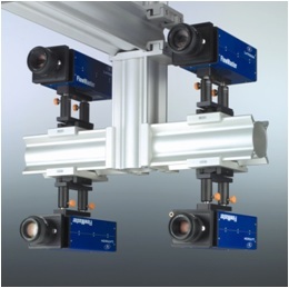
北京欧兰科技发展有限公司为您提供《空气和液体流场中3D3C 全体积速度矢量场检测方案(粒子图像测速)》,该方案主要用于其他中3D3C 全体积速度矢量场检测,参考标准--,《空气和液体流场中3D3C 全体积速度矢量场检测方案(粒子图像测速)》用到的仪器有体视层析粒子成像测速系统(Tomo-PIV)、Imager sCMOS PIV相机
推荐专场


相关方案
更多
该厂商其他方案
更多