微流体中混合效果检测方案(粒子图像测速)

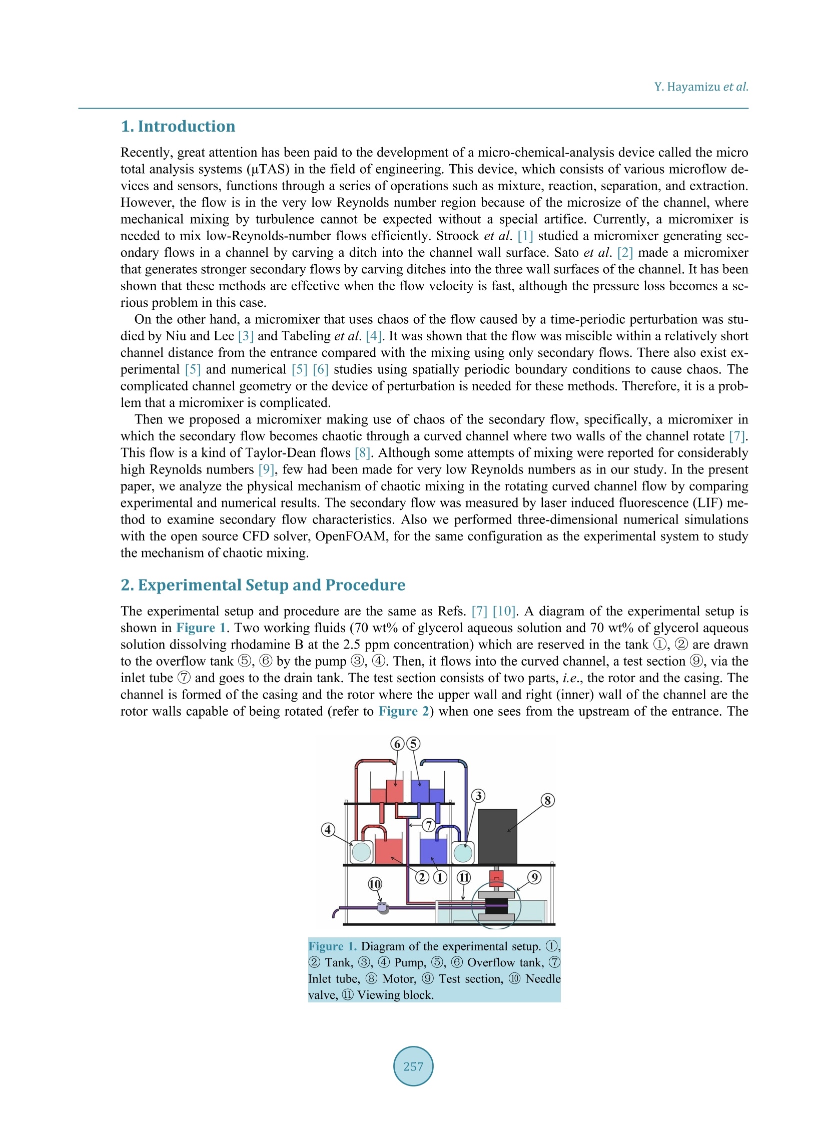
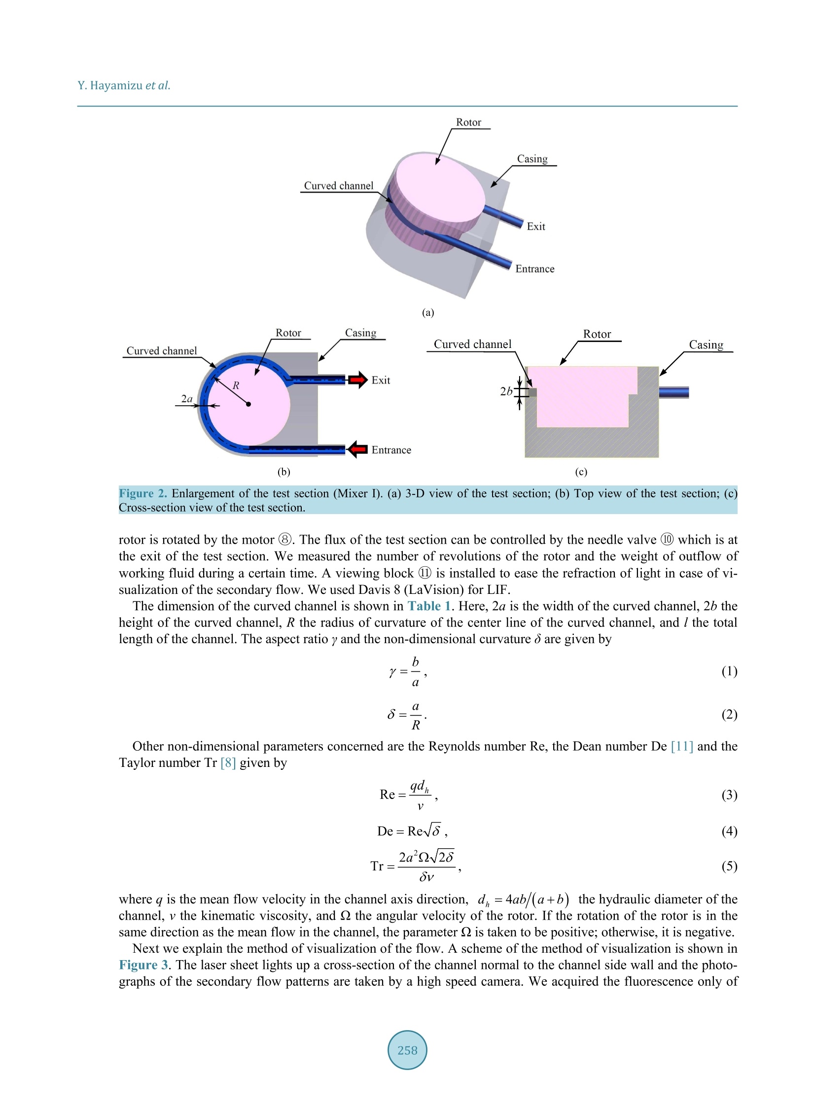
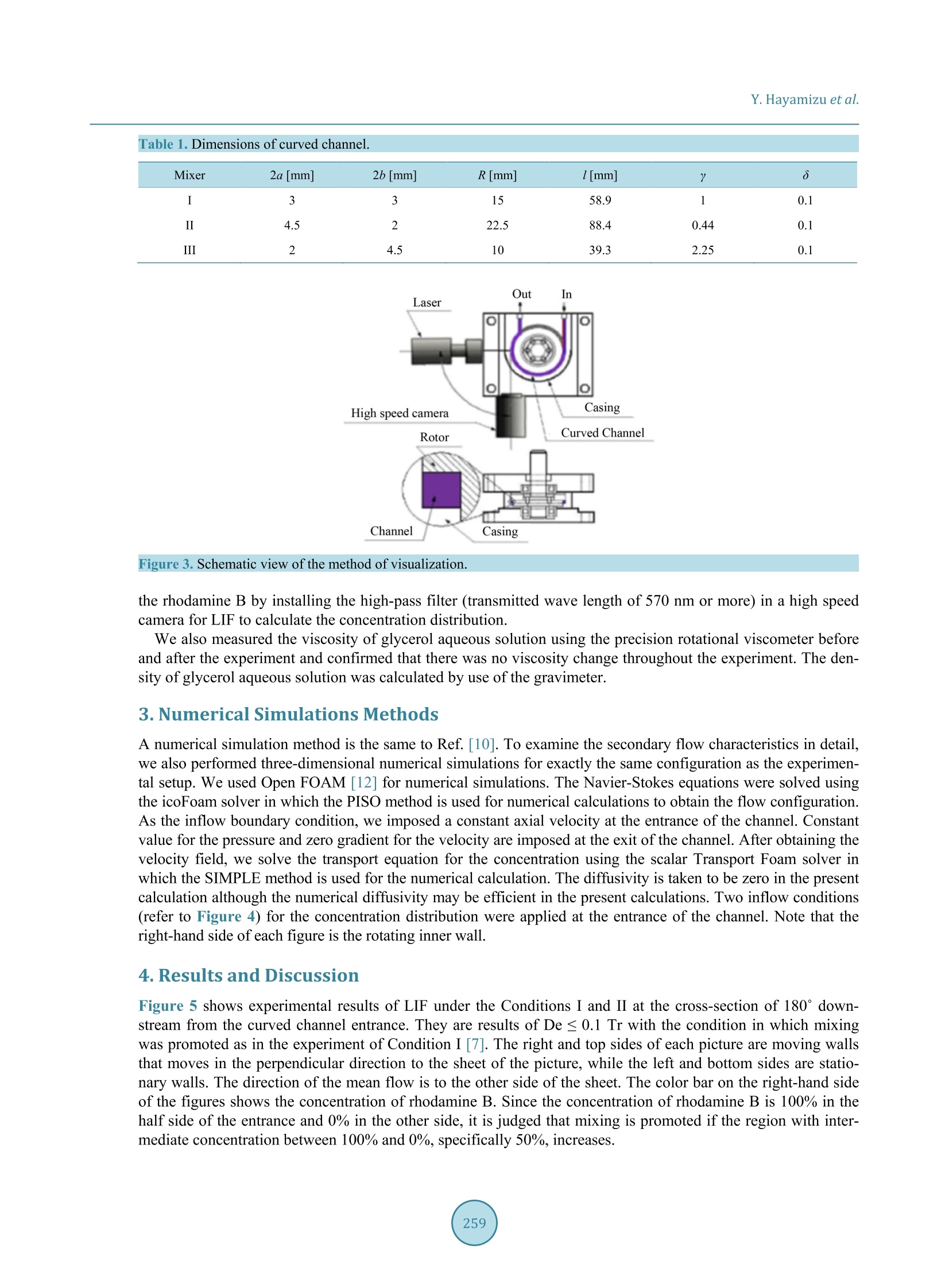
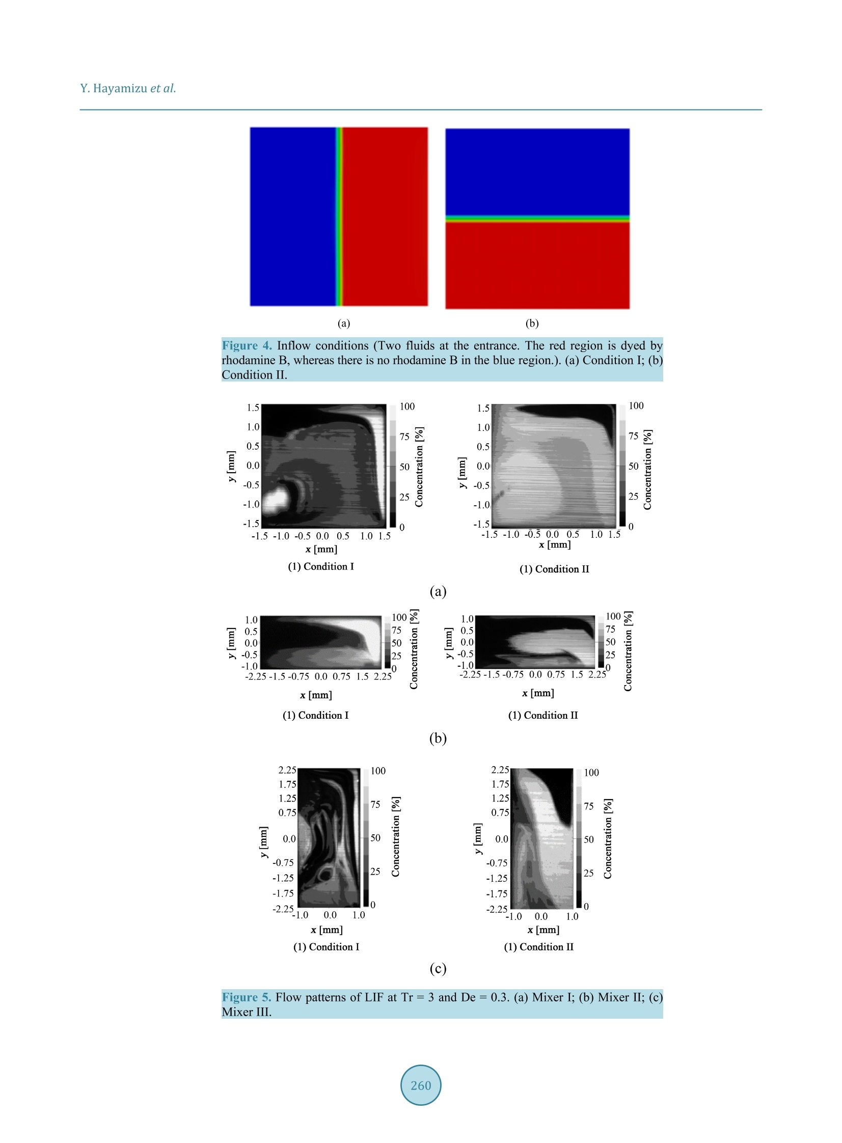
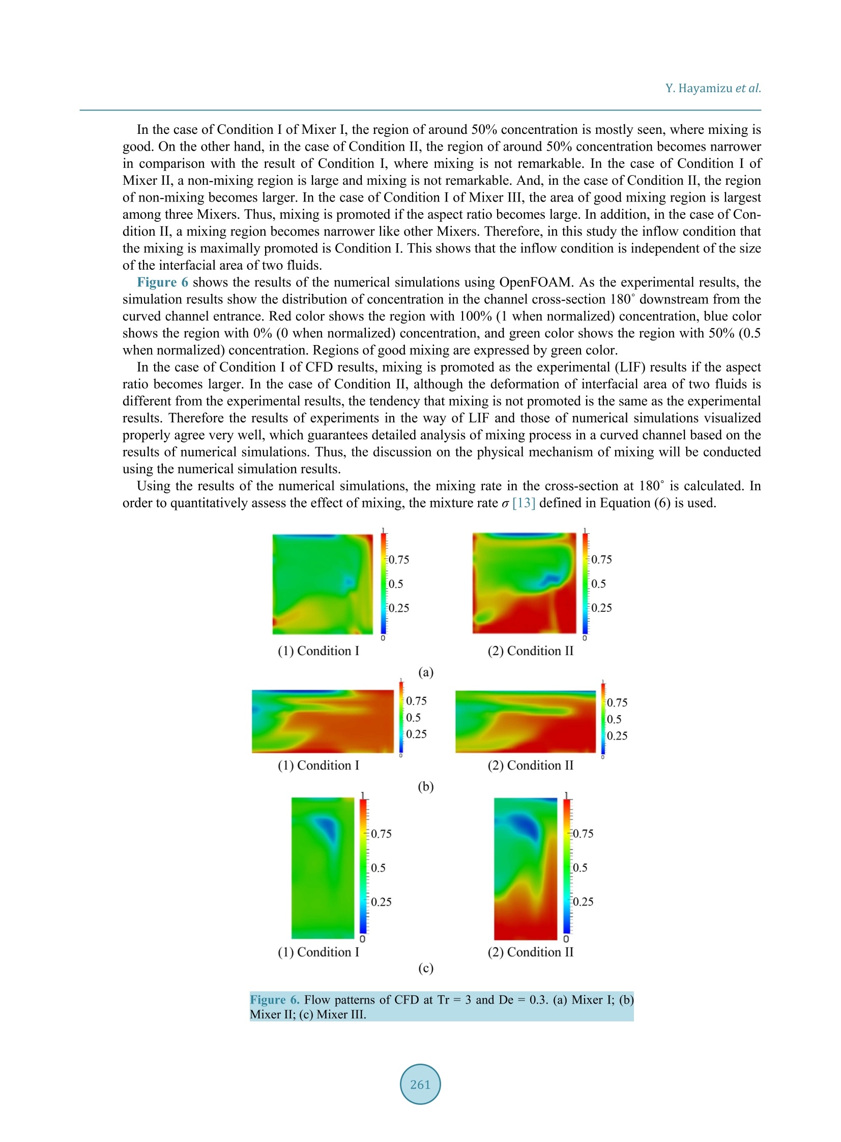
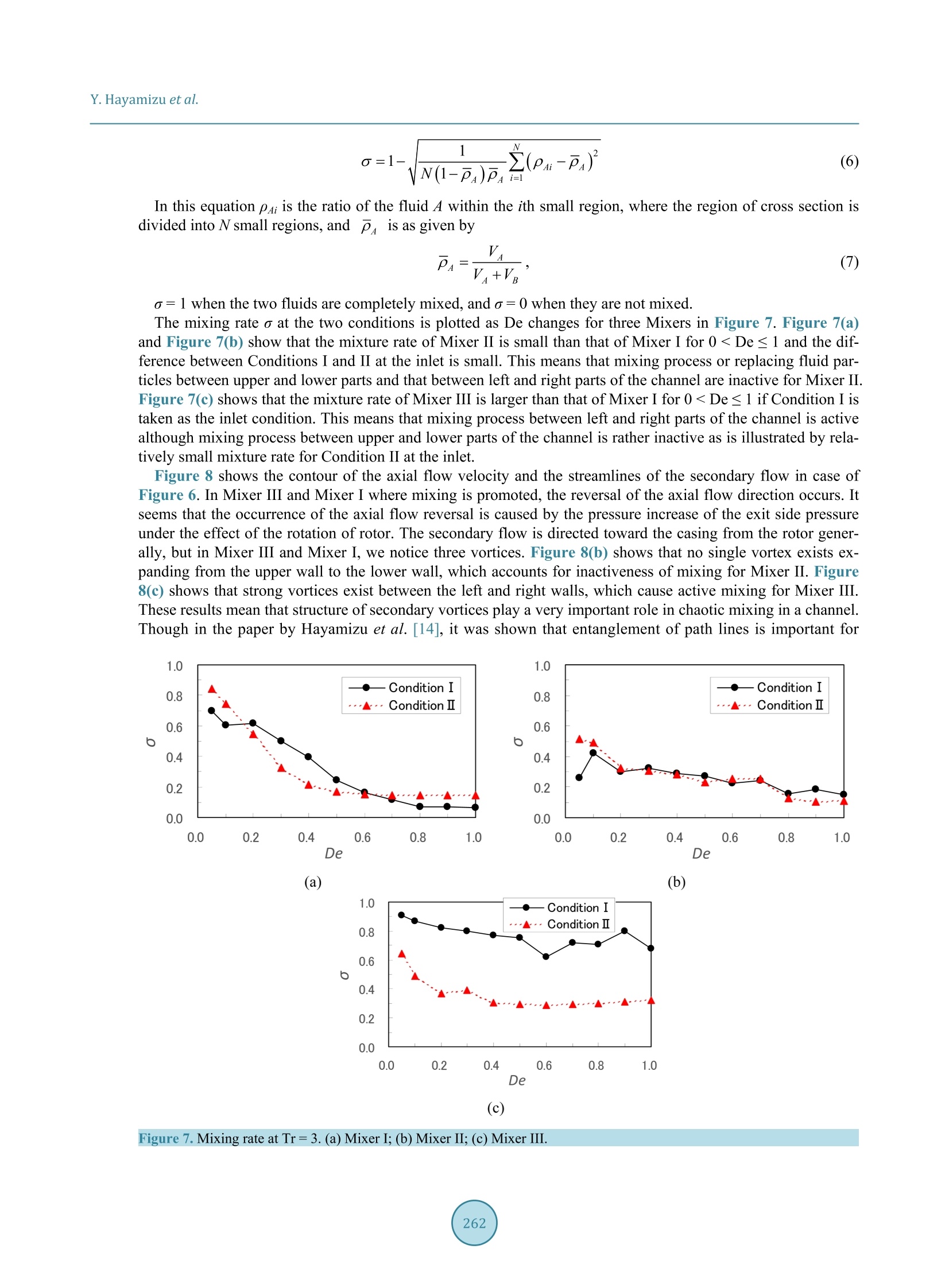
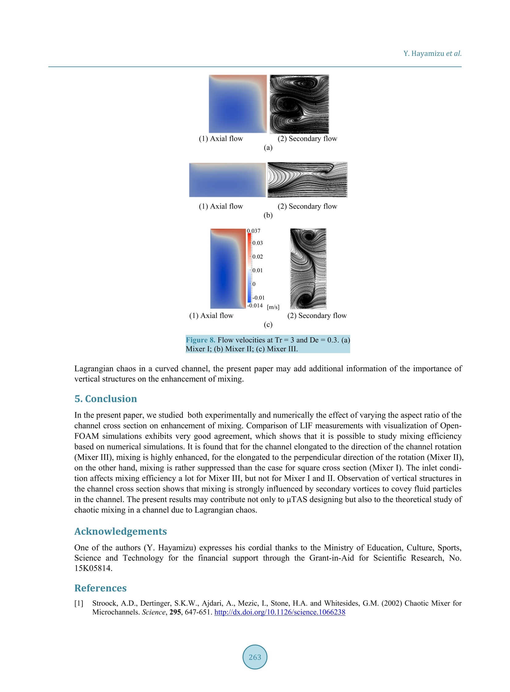
Open Journal of Fluid Dynamics，2015， 5， 256-264Published Online September 2015 in SciRes. http：//www.scirp.org/journal/ojfdhttp：//dx.doi.org/10.4236/ojfd.2015.53027 Y. Hayamizu et al. A Micromixer Using the Taylor-Dean Flow：Effects of Aspect Ratio and InflowCondition on the Mixing Yasutaka Hayamizu1， Toshihiko Kawabe2， Shinichiro Yanase3， Takeshi Gonda1，Shinichi Morita1， Shigeru Ohtsuka1，Kyoji Yamamoto Department of Mechanical Engineering， Yonago National College of Technology， Tottori， JapanTechnical Division， Tsurumi Manufacturing Co.， Ltd.， Tottori， JapanGraduate School of Natural Science and Technology， Okayama University，Okayama，JapanEmail： hayamizu@yonago-k.ac.jp Received 20 August 2015； accepted 26 September 2015； published 29 September 2015 Copyright C 2015 by authors and Scientific Research Publishing Inc. Abstract Chaotic mixing in three different types of curved-rectangular channels flow has been studied ex-perimentally and numerically. Two walls of the channel (inner and top walls) rotate around thecenter of curvature and a pressure gradient are imposed in the direction toward the exit of thechannel. This flow is a kind of Taylor-Dean flow. There are two parameters dominating the flow，the Dean number De (cc the pressure gradient or the Reynolds number) and the Taylor number Tr(oc the angular velocity of the wall rotation). In this paper， we analyze the physical mechanism ofchaotic mixing in the Taylor-Dean flow by comparing experimental results and numerical ones.We produced three micromixer models of the curved channel， several centimeters long， with rec-tangular cross-section of a few millimeters side. The secondary flow is measured using laser in-duced fluorescence (LIF) method to examine secondary flow characteristics. Also we performedthree-dimensional numerical simulations with the open source CFD solver， OpenFOAM， for thesame configuration as the experimental system to study the mechanism of chaotic mixing. It isfound that good mixing performance is obtained in the case of De ≤0.1 Tr， and it becomes moreremarkable when the aspect ratio tends to large. And it is found that the mixing efficiency changesaccording to the aspect ratio and inflow condition. Keywords Component， Taylor-Dean Flow， Chaotic Mixing， Secondary Flow， LIF， CFD ( How to cite this paper： H ayamizu，Y.， K a wabe， T.， Yanase， S.， Gonda， T.， Morita， S.， Ohtsuka，S. and Yamamoto， K. ( 2015) AMicromixer Using th e Taylor-Dean Flow： Effects of Aspect Rati o and Inflow Condi t ion on the Mixing. Open Journal of Fluid Dynamics，5，256-264.ht t p ： //dx.doi.org/10.4236/ojfd. 2 01 5 .53027 ) 1.Introduction Recently， great attention has been paid to the development of a micro-chemical-analysis device called the micrototal analysis systems (uTAS) in the field of engineering. This device， which consists of various microflow de-vices and sensors， functions through a series of operations such as mixture， reaction， separation， and extraction.However， the flow is in the very low Reynolds number region because of the microsize of the channel， wheremechanical mixing by turbulence cannot be expected without a special artifice. Currently， a micromixer isneeded to mix low-Reynolds-number flows efficiently. Stroock et al.[1] studied a micromixer generating sec-ondary flows in a channel by carving a ditch into the channel wall surface. Sato et al. [2] made a micromixerthat generates stronger secondary flows by carving ditches into the three wall surfaces of the channel. It has beenshown that these methods are effective when the flow velocity is fast， although the pressure loss becomes a se-rious problem in this case. On the other hand， a micromixer that uses chaos of the flow caused by a time-periodic perturbation was stu-died by Niu and Lee [3] and Tabeling et al. [4]. It was shown that the flow was miscible within a relatively shortchannel distance from the entrance compared with the mixing using only secondary flows. There also exist ex-perimental [5] and numerical [5] [6] studies using spatially periodic boundary conditions to cause chaos. Thecomplicated channel geometry or the device of perturbation is needed for these methods. Therefore， it is a prob-lem that a micromixer is complicated. Then we proposed a micromixer making use of chaos of the secondary flow， specifically， a micromixer inwhich the secondary flow becomes chaotic through a curved channel where two walls of the channel rotate [7].This flow is a kind of Taylor-Dean flows [8]. Although some attempts of mixing were reported for considerablyhigh Reynolds numbers [9]， few had been made for very low Reynolds numbers as in our study. In the presentpaper， we analyze the physical mechanism of chaotic mixing in the rotating curved channel flow by comparingexperimental and numerical results. The secondary flow was measured by laser induced fluorescence (LIF) me-thod to examine secondary flow characteristics. Also we performed three-dimensional numerical simulationswith the open source CFD solver， OpenFOAM， for the same configuration as the experimental system to studythe mechanism of chaotic mixing. 2. Experimental Setup and Procedure The experimental setup and procedure are the same as Refs. [7] [10]. A diagram of the experimental setup isshown in Figure 1. Two working fluids (70 wt% of glycerol aqueous solution and 70 wt% of glycerol aqueoussolution dissolving rhodamine B at the 2.5 ppm concentration) which are reserved in the tank ①，②are drawnto the overflow tank ⑤， ⑥ by the pump ③， ④. Then， it flows into the curved channel， a test section ⑨， via theinlet tube ⑦ and goes to the drain tank. The test section consists of two parts， i.e.， the rotor and the casing. Thechannel is formed of the casing and the rotor where the upper wall and right (inner) wall of the channel are therotor walls capable of being rotated (refer to Figure 2) when one sees from the upstream of the entrance. The (a) (b) (c) Figure 2. Enlargement of the test section (Mixer I).(a) 3-D view of the test section； (b) Top view of the test section； (c)Cross-section view of the test section. rotor is rotated by the motor ⑧. The flux of the test section can be controlled by the needle valve ① which is atthe exit of the test section. We measured the number of revolutions of the rotor and the weight of outflow ofworking fluid during a certain time. A viewing block ① is installed to ease the refraction of light in case of vi-sualization of the secondary flow. We used Davis 8(LaVision) for LIF. The dimension of the curved channel is shown in Table 1. Here， 2a is the width of the curved channel， 2b theheight of the curved channel， R the radius of curvature of the center line of the curved channel， and I the totallength of the channel. The aspect ratio y and the non-dimensional curvature o are given by Other non-dimensional parameters concerned are the Reynolds number Re， the Dean number De [11] and theTaylor number Tr [8] given by where q is the mean flow velocity in the channel axis direction， d=4ab(a+b) the hydraulic diameter of thechannel， v the kinematic viscosity， and Q the angular velocity of the rotor. If the rotation of the rotor is in thesame direction as the mean flow in the channel， the parameter Q is taken to be positive； otherwise， it is negative. Next we explain the method of visualization of the flow. A scheme of the method of visualization is shown inFigure 3. The laser sheet lights up a cross-section of the channel normal to the channel side wall and the photo-graphs of the secondary flow patterns are taken by a high speed camera. We acquired the fluorescence only of Mixer 2a [mm] 2b[mm] R [mm 7 [mm] 3 3 15 58.9 0.1 I 4.5 2 22.5 88.4 0.44 0.1 11 2 4.5 10 39.3 2.25 0.1 Figure 3. Schematic view of the method of visualization. the rhodamine B by installing the high-pass filter (transmitted wave length of 570 nm or more) in a high speedcamera for LIF to calculate the concentration distribution. We also measured the viscosity of glycerol aqueous solution using the precision rotational viscometer beforeand after the experiment and confirmed that there was no viscosity change throughout the experiment. The den-sity of glycerol aqueous solution was calculated by use of the gravimeter. 3.Numerical Simulations Methods A numerical simulation method is the same to Ref. [10]. To examine the secondary flow characteristics in detail，we also performed three-dimensional numerical simulations for exactly the same configuration as the experimen-tal setup. We used Open FOAM [12] for numerical simulations. The Navier-Stokes equations were solved usingthe icoFoam solver in which the PISO method is used for numerical calculations to obtain the flow configuration.As the inflow boundary condition， we imposed a constant axial velocity at the entrance of the channel. Constantvalue for the pressure and zero gradient for the velocity are imposed at the exit of the channel. After obtaining thevelocity field， we solve the transport equation for the concentration using the scalar Transport Foam solver inwhich the SIMPLE method is used for the numerical calculation. The diffusivity is taken to be zero in the presentcalculation although the numerical diffusivity may be efficient in the present calculations. Two inflow conditions(refer to Figure 4) for the concentration distribution were applied at the entrance ofthe channel. Note that theright-hand side of each figure is the rotating inner wall. 4. Results and Discussion Figure 5 shows experimental results of LIF under the Conditions I and II at the cross-section of 180° down-stream from the curved channel entrance. They are results of De ≤ 0.1 Tr with the condition in which mixingwas promoted as in the experiment of Condition I [7]. The right and top sides of each picture are moving wallsthat moves in the perpendicular direction to the sheet of the picture， while the left and bottom sides are statio-nary walls. The direction of the mean flow is to the other side of the sheet. The color bar on the right-hand sideof the figures shows the concentration of rhodamine B. Since the concentration of rhodamine B is 100% in thehalf side of the entrance and 0% in the other side， it is judged that mixing is promoted if the region with inter-mediate concentration between 100% and 0%， specifically 50%， increases. (a) (b) Figure 4. Inflow conditions (Two fluids at the entrance. The red region is dyed byrhodamine B， whereas there is no rhodamine B in the blue region.). (a) Condition I； (b)Condition II. Figure 5. Flow patterns of LIF at Tr=3and De =0.3. (a) Mixer I； (b) Mixer ⅡI； (c)Mixer III. In the case of Condition I of Mixer I， the region of around 50% concentration is mostly seen， where mixing isgood. On the other hand， in the case of Condition II， the region of around 50% concentration becomes narrowerin comparison with the result of Condition I， where mixing is not remarkable. In the case of Condition I ofMixer II， a non-mixing region is large and mixing is not remarkable. And， in the case of Condition II， the regionof non-mixing becomes larger. In the case of Condition I of Mixer III， the area of good mixing region is largestamong three Mixers. Thus， mixing is promoted if the aspect ratio becomes large. In addition， in the case of Con-dition II， a mixing region becomes narrower like other Mixers. Therefore， in this study the inflow condition thatthe mixing is maximally promoted is Condition I. This shows that the inflow condition is independent of the sizeof the interfacial area of two fluids. Figure 6 shows the results of the numerical simulations using OpenFOAM. As the experimental results， thesimulation results show the distribution of concentration in the channel cross-section 180° downstream from thecurved channel entrance. Red color shows the region with 100% (1 when normalized) concentration， blue colorshows the region with 0% (0 when normalized) concentration， and green color shows the region with 50% (0.5when normalized) concentration. Regions of good mixing are expressed by green color. In the case of Condition I of CFD results， mixing is promoted as the experimental (LIF) results if the aspectratio becomes larger. In the case of Condition II， although the deformation of interfacial area of two fluids isdifferent from the experimental results， the tendency that mixing is not promoted is the same as the experimentalresults. Therefore the results of experiments in the way of LIF and those of numerical simulations visualizedproperly agree very well， which guarantees detailed analysis of mixing process in a curved channel based on theresults of numerical simulations. Thus， the discussion on the physical mechanism of mixing will be conductedusing the numerical simulation results. Using the results of the numerical simulations， the mixing rate in the cross-section at 180° is calculated. Inorder to quantitatively assess the effect of mixing， the mixture rate a [13] defined in Equation (6) is used. Figure 6. Flow patterns of CFD at Tr=3 and De=0.3. (a) Mixer I； (b)Mixer II； (c) Mixer II. In this equation pAi is the ratio of the fluid A within the ith small region， where the region of cross section isNcm11divided into N small regions， and pis as given by o=1 when the two fluids are completely mixed， and s=0 when they are not mixed. The mixing rate o at the two conditions is plotted as De changes for three Mixers in Figure 7. Figure 7(a)and Figure 7(b) show that the mixture rate of Mixer II is small than that of Mixer I for 0

确定