


方案详情
文
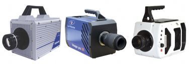
激光器采用Quantronix 双腔高重复率激光器。单脉冲能量25 mJ @ 1 kHz。系统配备6台Photron CMOS 相机。满帧分辨率1024 x 1024像素。
方案详情

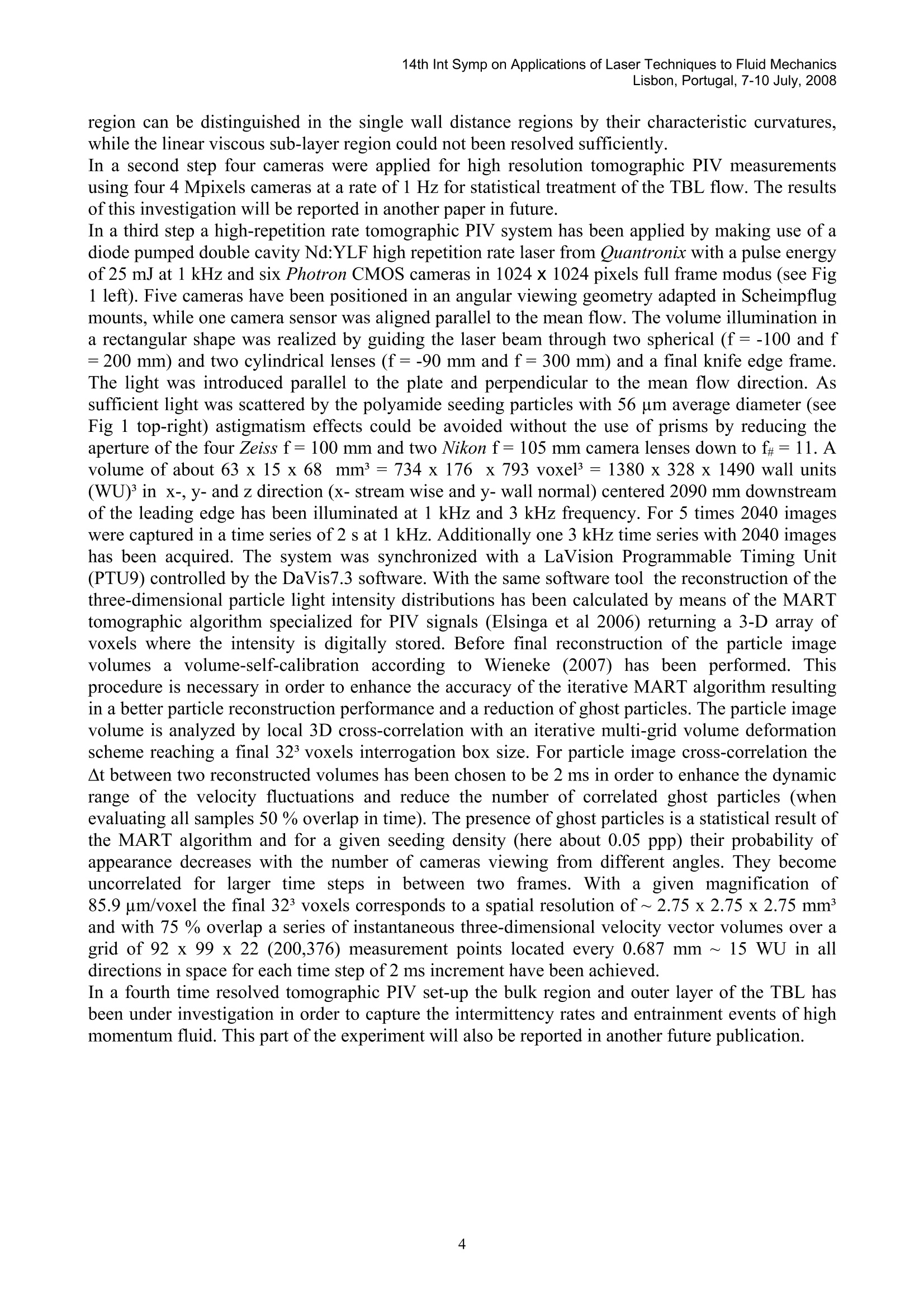
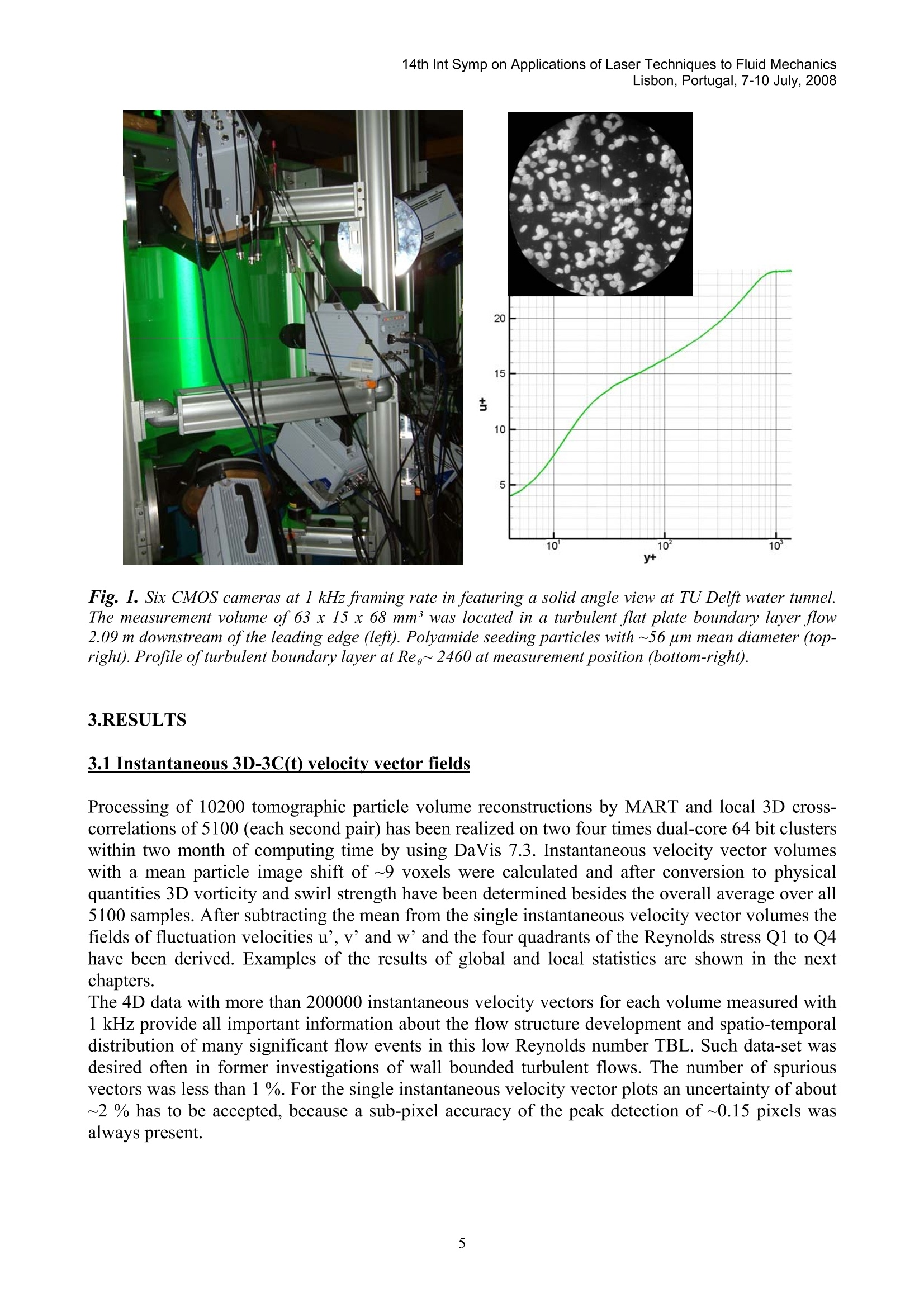
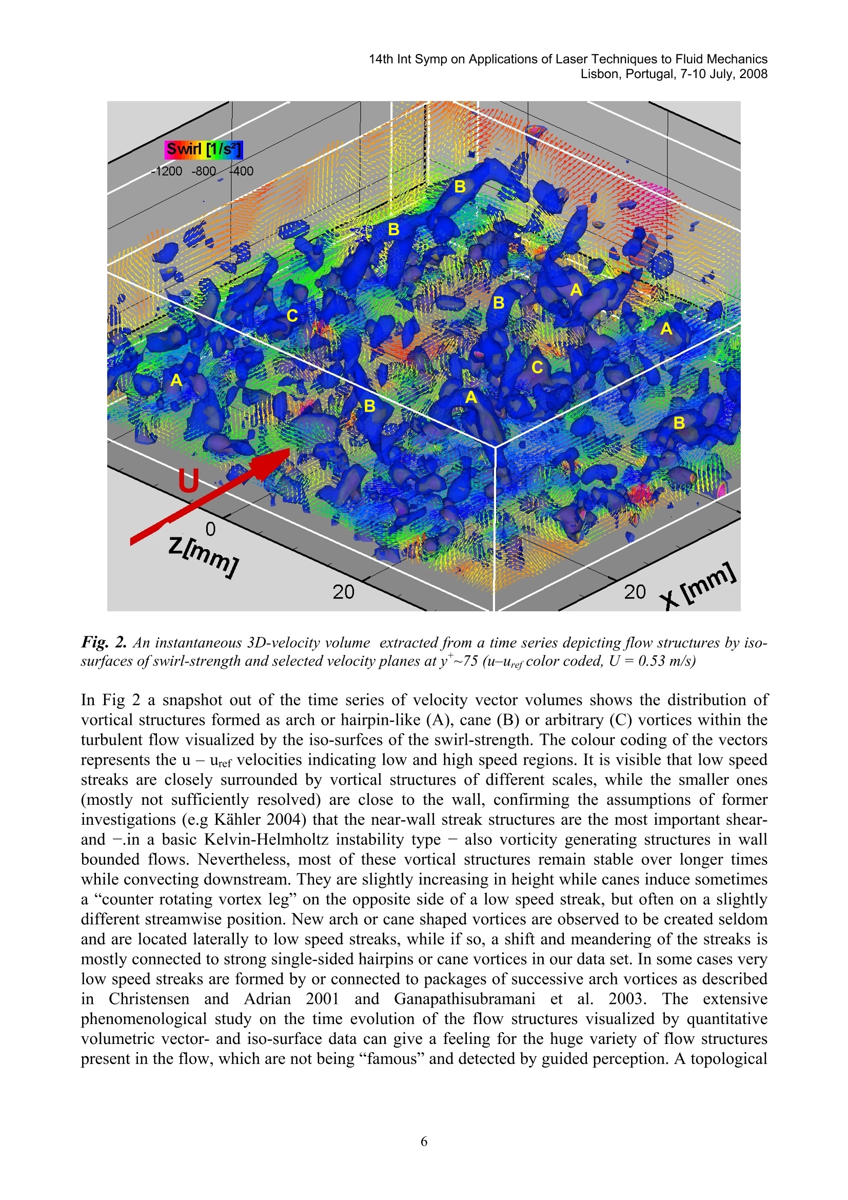
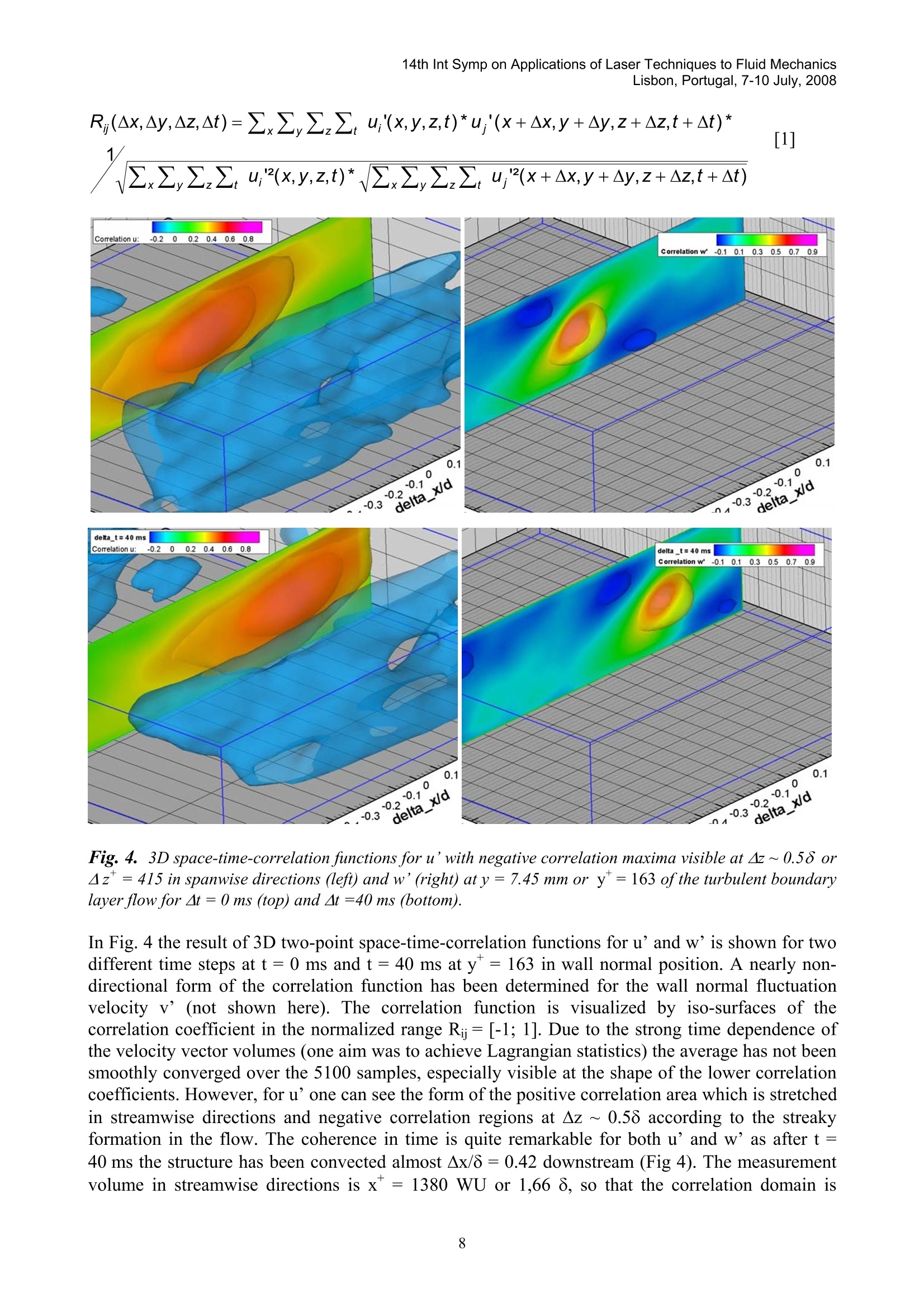
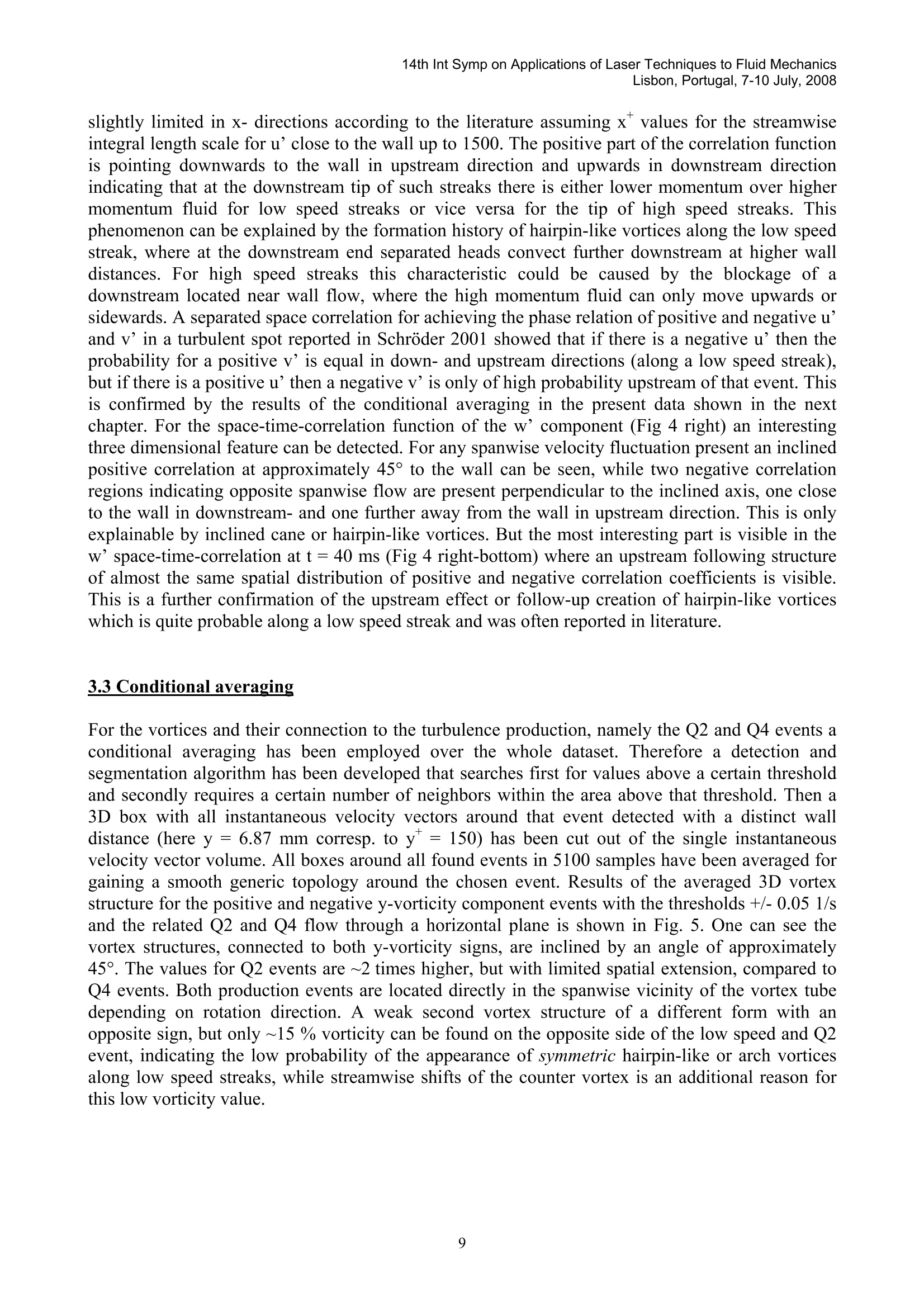
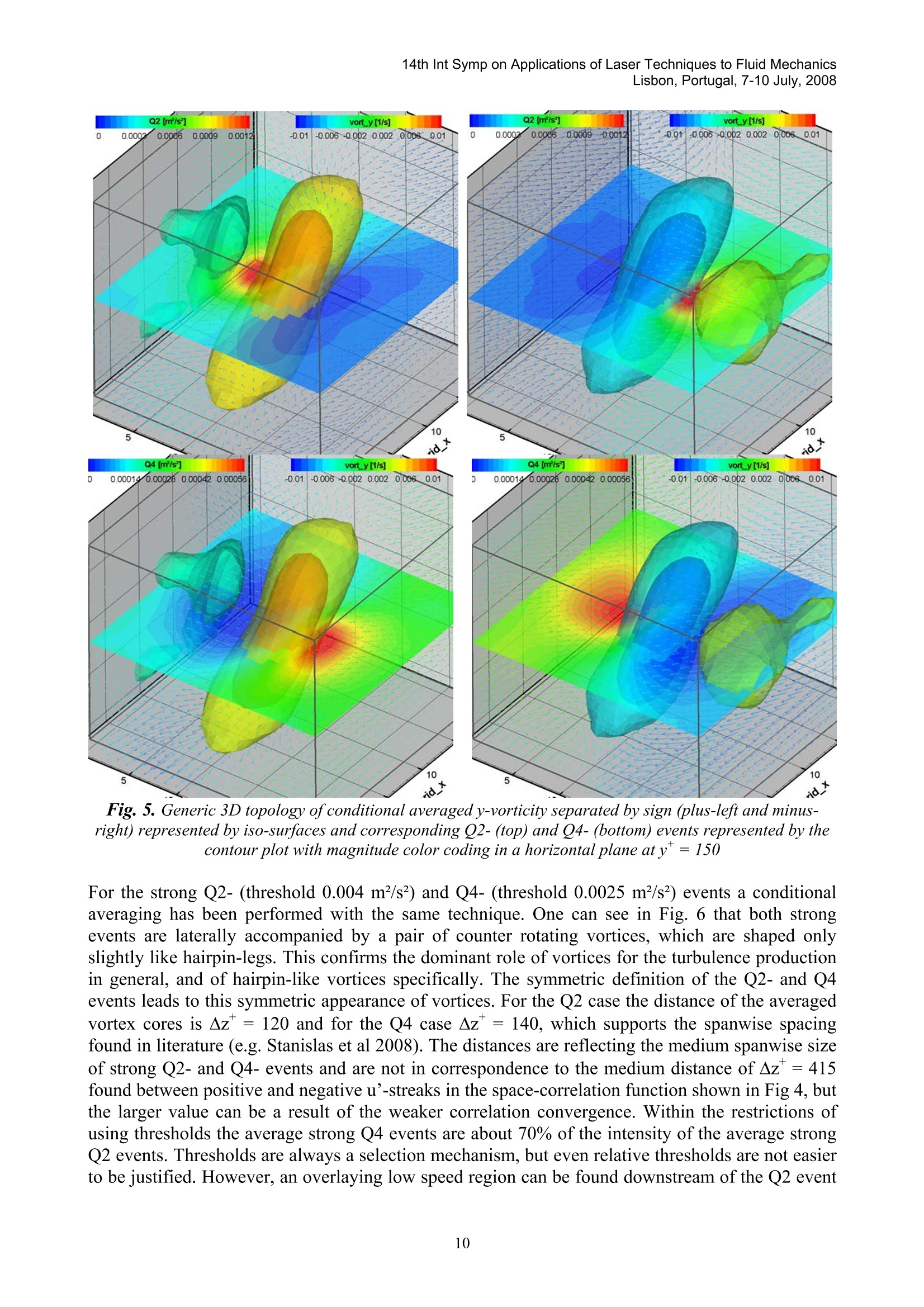
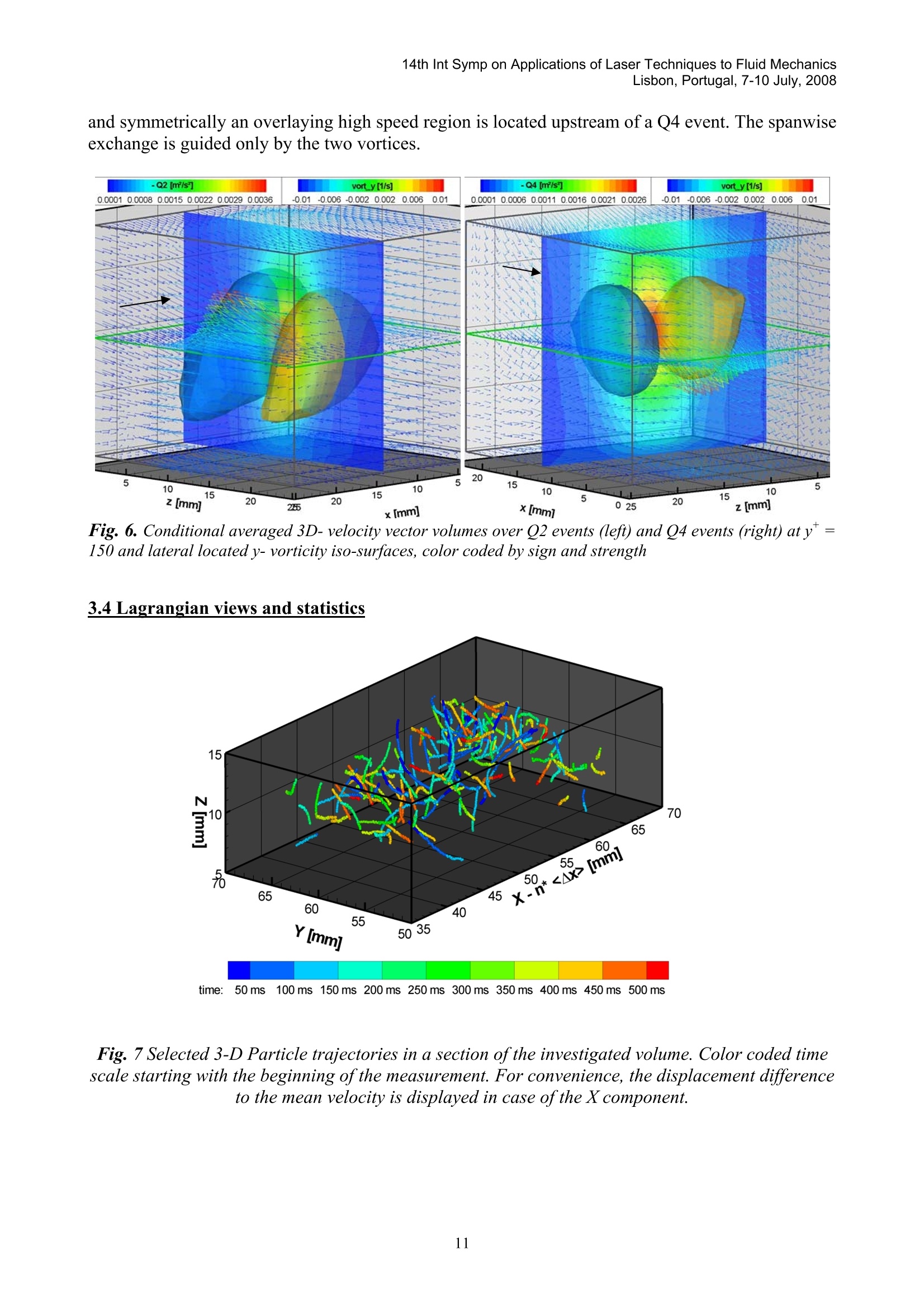
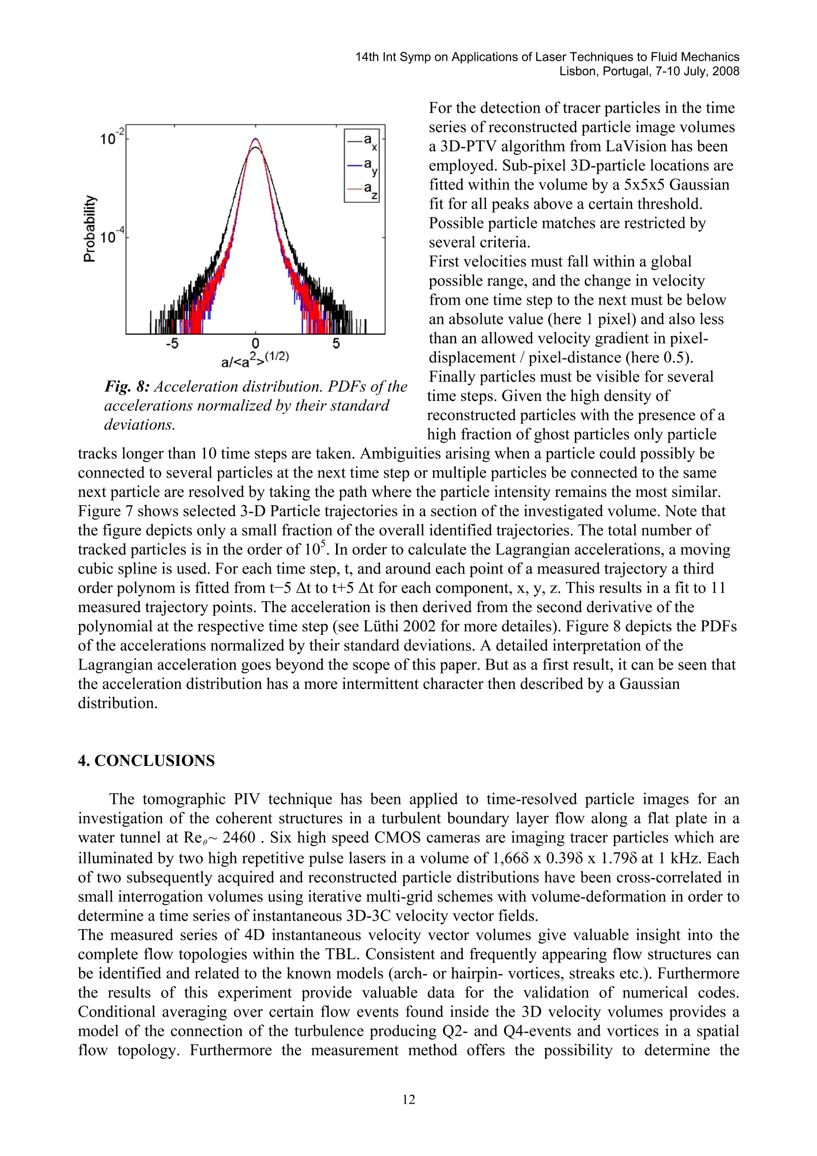
14th Int Symp on Applications of Laser Techniques to Fluid MechanicsLisbon, Portugal, 7-10 July, 2008 Lagrangian and Eulerian views into a turbulent boundary layer flowusing time-resolved tomographic PIV A. Schroder,R. Geisler,K. Staack, B. Wieneke, G.E. Elsinga, F. Scarano, A. Henning* 1: Deutsches Zentrum fir Luft- und Raumfahrt, Institut f. Aerodynamik und Stromungstechnik, Bunsenstrasse 10, 37073 Gottingen, Germany, email: andreas.schroeder@dlr.de,reinhard.geisler@dlr.de2: La Vision GmbH, Anna-Vandenhoeck-Ring 19, 37081 Gottingen, Germany, email: bwieneke@lavision.de 3: Delft University of Technology, Department of Aerospace Engineering, Kluyverweg 1, 2629HS, Delft, TheNetherlands, emails: g.e.elsinga@tudelft.nl,f.scarano@tudelft.nl 4: Technical University Berlin. Current address: Deutsches Zentrum fiir Luft- und Raumfahrt, Institut f. Aerodynamikund Stromungstechnik, Bunsenstrasse 10, 37073 Gottingen, Germany Abstract The momentum exchange mechanisms in a turbulent boundary layer (TBL) flow are of manifoldtemporal and spatial scales and governed by the organization of self-sustaining coherent flow structuresdriven by entrained high momentum fluid. Generic flow structures such as hairpin-like vortices and spanwisealternating wall bounded low- and high-speed streaks have been observed and extensively analyzed withboth experimental and numerical methods, e.g. by means of PIV (Christensen & Adrian 2001, Kahler 2004,Stanislas et al. 2008) or DNS (Spalart 1988, Robinson 1991, Kang et al. 2007). In many studies the role ofthese structures for the wall normal and spanwise fluid exchange has been highlighted mostly within anEulerian reference frame. But for a full understanding of the momentum exchange in turbulent wall flows astep towards a spatially resolved Lagrangian frame of reference would be advantageous. The data achieved from the present application of time-resolved tomographic PIV to a flat plate turbulentboundary layer flow in a water tunnel at Reo~ 2460 enables for the first time a topological investigation ofthe flow structures and related particle motions within a temporally and spatially highly resolved Lagrangianand Eulerian reference frame. 1.INTRODUCTION In the turbulence flow research community ttwWo obranches can be distinguished which reflects thetwo general view points either with a more or less application driven focus on shear- and wallbounded turbulence or with a more fundamental research driven interest in s.c. homogeneous,isotropic turbulence. In the isotropic turbulence branch Lagrangian statistics on temporally highlyresolved trajectories of few single spatially independent tracer particles in the flow using differentPTV techniques are dominant on the experimental side, while in the shear- and wall boundedturbulence research Eulerian reference frame approaches using PIV or hot-wire probe techniquesbecame dominant leading to concepts and models of coherent structures as the main carriers ofturbulent fluid exchange. This branch development seems to be quite natural as in shear flows theintrinsic turbulent dissipation scale e and therefore the Kolmogorov scales n and tn are dependingon the position in space resp. wall distance for TBL, while they are universal in isotropic turbulencemaking assumptions on highest levels of generality possible relying on high performance DNS data(Yeung 2002, Biferale et al. 2006). However, experiments measuring turbulent flows inaLagrangian reference frame need techniques which allow following the trajectory of (single)particles in a high temporal resolution comparable to the smallest turbulence time scales and at thesame experiment also for a long observation time in order to cover also the integral time scales. Upto now the experimental Lagrangian turbulence characterization has been performed by statisticalanalysis over several spatially independent single or groups of particles measured by trackingmethods (Virant & Dracos 1997,Mordant et al. 2007). Using these techniques the achieved spatial resolution did not allow describing the coherent structures. One of the challenges of experimentalturbulence research is therefore the combination of both viewpoints in a single experiment. Ofcourse complete DNS and specific research topics like particle dispersion in boundary layers, two-phase flows etc. are bridging always both reference frames, but up to now no measurementtechnique was available which enables the possibility to capture at the same time both properties ofthe flow field in a high spatial and temporal resolution. In the past two decades considerable experimental and numerical work on coherent structures inwall bounded turbulent flows has been carried out. A focus for a direct comparison of the results ofthe present work will be the spatio-temporal models of coherent flow structures,which have beendeveloped partly by using the PIV techniques (e.g. Robinson 1991; Meinhart 1994; Schoppa andHussain 1997; Tomkins et al. 2003 and Kahler 2004). Since almost two decades the PIV techniquehas enabled the determination of instantaneous velocity vector fields in a plane of the flow,returning important results based on instantaneous and statistical approaches to the analysis of theturbulent flow structures. Successful extensions of PIV experiments towards dual plane and/or timeresolution have been performed during that time and their applications to turbulent flowsemphasized the role of coherent flow structures for this research field. In a recent paper Stanislas etal. 2008 described the scaling properties, topologies and distribution functions of rbulent boundary layer for two diRvortices in atueffferent Reynolds numbers at Res=7800 and Res=15000 byusing conditional averaging and space correlation functions. They found in accordance to earlierPIV measurements by Kahler 2004 that hairpin like vortices are dominantly one sided and caneshaped, and then play a major role for the spatial organization of wall normal and spanwise flowexchange. They are apparently connected to the turbulence production events, the (instantaneous)negative Reynolds stresses u’v', so called Q2- and Q4- events in the buffer and log layer.Equilibrium between production and dissipation can be assumed for the log layer. The main aim ofStanislas et al. paper is to show the possibility of a universal scaling of wall turbulence by Ue andthe Kolmogorov scale n. Diorio et al. 2007 are reporting about the results of multi hot wire measurements in a TBL. The dataenables them to reconstruct the average spatial neighbourhood of dissipation and productionregions. They claim to identify the highest instantaneous dissipation rates within the vortex lines ofe.g. a hairpin leg, while the highest production rates are located in both spanwise vicinities as Q2and Q4 events. In the results chapter of the present paper conditional averaging of our data at Q2and Q4 events and the two signs of y-vorticity will return a generic 3D velocity vector topology ofthese neighbourhood relations (see Fig 7, 8). A recent application of the tomographic PIV technique to a tripped turbulent boundary layer flow ata low Reynolds number has been reported by Elsinga et al. 2007. In their paper instantaneousspatial topologies of the coherent structures like hairpin vortices, packets of hairpins along lowspeed streaks and Q2- events have been visualized segmented in 3D quantitatively with a very highquality. The coherent structures have been extensively described and global statistics have beencalculated for comparison with theory and literature. The first time preliminary results of time-resolved 3D-3C velocity vector fields from turbulent wall bounded flows in air gained by usingtomographic PIV have been published by Schroder et al in 2006. The turbulent mixing due to the Q-2-and Q-4-events, has been found to be connected to a staggeredpattern of hairpin-like vortices, see idealized mixer-model of substructure formation inside aturbulent spot from Schroder and Kompenhans 2004 or in TBL from Elsinga et al. 2007. Schroder2001 concluded an interpretation of spatial distributions of space-time correlations of the singleReynolds stress elements calculated for different planes parallel to the wall that the initial processfor the formation of hairpin vortices seems to be a Q4-event which was deflected by a downstreamflow structure and transformed into a Q-3 event with additional spanwise flow variance, which theninteracts with a wall-near low speed streak. Such events have been found in the 3D-3C and timeresolved data of Schroder et al. 2008, but could not be confirmed yet as an essential mechanism. It will be shown that the data-set achieved by time-resolved tomographic PIV in the presented workgives valuable insight into the four-dimensional flow organization and exchange mechanisms ofcoherent flow structures inside a fully developed flat plate turbulent boundary layer with zeropressure gradients at Re~ 2460. For the first time we can expect flow information from bothreference frames: Eulerian and Lagrangian. A topological analysis by means of 3D space-(time)-correlations, PDF’s of different scalars, conditional averaging and time series of instantaneousvelocity vector volumes on one side and PDF’s of Lagrangian accelerations and a view of particletracks are the results presented in this paper. The Lagrangian time-scales towards integral values areof course limited by the finite extent of the measurement volume, the restrictions of the PTValgorithm in finding long paths and the overall convection velocity. On the other hand the very hightime sampling rate allows to fully resolve the flow for the Kolmogorov time scales, which havebeen estimated from derivatives of the instantaneous u-velocity in x-directions between tn=15 to40 ms within the measurement volume depending on the wall distance. After tomographicreconstruction of a time series of particle image recordings in volumes a PTV algorithm fromLaVision has been employed enabling to describe the motion of several thousands of particles in aLagrangian frame of reference within the measurement volume. This approach allows thecalculation of the wall distance dependencies of the PDF’s of Lagrangian accelerations and a closeexamination of the momentum exchange processes. Time series of instantaneous 3D velocity vectorfields have been determined, while 3D-vorticity and swirling strength fields are represented by iso-surfaces, which highlight the topology of individual vortical substructures, their time developmentand induced flow. Swirling strength is the imaginary part of the locally calculated complexeigenvalue of the velocity gradient tensor, which is a measure for rotation excluding shear vorticity(Zhou et al. 1999). It has to be mentioned that the relatively coarse spatial grid resolution for thebuffer and log-layer region in the measurement volume emphasizes the bigger vortical structures,but nevertheless the main topologies like hairpin-like vortices and low and high speed streaks havebeen sufficiently resolved. 2. EXPERIMENTAL SET-UP AND PROCEDURE The experiments have been conducted in the water tunnel at TU Delft where a turbulentboundary layer flow has been established along a vertical mounted flat acrylic glass plate at a freestream velocity of 0.53 m/s. The plate dimensions are 250 x 80 cm² and an elliptic leading edge wasemployed, while a zero pressure gradient has been adapted by a trailing edge flap. The flow on theobservation side was tripped by a spanwise attached zig-zag band 150 mm downstream of theleading edge resulting in a thickness of the turbulent boundary layer of 38 mm corresponding toRe,~2460 based on momentum thickness at the measurement volume. The temperature wascontrolled and hold constant, while the turbulence level of the free stream velocity was below0.5%. For the general characterization of the boundary layer flow a f=105 mm lens from Nikonhas been used for a high resolution 2C-PIV experiment with a low-repetition rate system composedof a Big Sky CFR-200 laser of 200 mJ pulse energy and a LaVision Imager PRO-X camera of 4Mpixels. One thousand statistically independent double particle images in a region of ~ 50 x50 mm² have been evaluated by 8 x 8 pixels interrogation windows corresponding to a spatialresolution of 4.4 wall units in x- and y-direction in an ensemble correlation mode in order tocalculate a high resolution boundary layer profile averaged over all wall normal columns of thegained velocity vector field. The resulting semi logarithmic boundary layer profile calculated inwall units after applying the Klauser-method for skin friction velocity estimation is given in Fig 1(bottom-right). The skin friction velocity has been estimated by regression between y*= 44 andy*=200 to ur = 0.0219 m/s and the coefficient to cr= 0.00345. Buffer layer, log-layer and bulk region can be distinguished in the single wall distance regions by their characteristic curvatures,while the linear viscous sub-layer region could not been resolved sufficiently. In a second step four cameras were applied for high resolution tomographic PIV measurementsusing four 4Mpixels cameras at a rate of 1 Hz for statistical treatment of the TBL flow. The resultsof this investigation will be reported in another paper in future. In a third step a high-repetition rate tomographic PIV system has been applied by making use of adiode pumped double cavity Nd:YLF high repetition rate laser from Quantronix with a pulse energyof 25 mJ at 1 kHz and six Photron CMOS cameras in 1024 x 1024 pixels full frame modus (see Fig1 left). Five cameras have been positioned in an angular viewing geometry adapted in Scheimpflugmounts, while one camera sensor was aligned parallel to the mean flow. The volume illumination ina rectangular shape was realized by guiding the laser beam through two spherical (f=-100 and f=200 mm) and two cylindrical lenses (f=-90 mm and f=300 mm) and a final knife edge frame.The light was introduced parallel to the plate and perpendicular to the mean flow direction. Assufficient light was scattered by the polyamide seeding particles with 56 um average diameter (seeFig 1 top-right) astigmatism effects could be avoided without the use of prisms by reducing theaperture of the four Zeiss f= 100 mm and two Nikon f=105 mm camera lenses down to f=11. Avolume of about 63 x 15 x 68 mm3=734x 1766 x 793 voxel=1380x 328 x1490 wall units(WU)in x-,y-and z direction (x- stream wise and y- wall normal) centered 2090 mm downstreamof the leading edge has been illuminated at 1 kHz and 3 kHz frequency. For 5 times 2040 imageswere captured in a time series of2 s at 1 kHz. Additionally one 3 kHz time series with 2040 imageshas been acquired. The system was synchronized with a LaVision Programmable Timing Unit(PTU9)controlled by the DaVis7.3 software. With the same software tool the reconstruction of thethree-dimensional particle light intensity distributions has been calculated by means of the MARTtomographic algorithm specialized for PIV signals (Elsinga et al 2006) returning a 3-D array ofvoxels where the intensity is digitally stored. Before final reconstruction of the particle imagevolumes aVvolume-self-calibration according to Wieneke (2007) has been performed. Thisprocedure is necessary in order to enhance the accuracy of the iterative MART algorithm resultingin a better particle reconstruction performance and a reduction of ghost particles. The particle imagevolume is analyzed by local 3D cross-correlation with an iterative multi-grid volume deformationscheme reaching a final 323voxels interrogation box size. For particle image cross-correlation theAt between two reconstructed volumes has been chosen to be 2 ms in order to enhance the dynamicrange of the velocity fluctuations and reduce the number of correlated ghost particles (whenevaluating all samples 50% overlap in time). The presence of ghost particles is a statistical result ofthe MART algorithm and for a given seeding density (here about 0.05 ppp) their probability ofappearance decreases with the number of cameras viewing from different angles. They becomeuncorrelated for larger time steps in between two frames.With a given magnification of85.9 um/voxel the final 32 voxels corresponds to a spatial resolution of~ 2.75 x 2.75x 2.75 mm’and with 75 % overlap a series of instantaneous three-dimensional velocity vector volumes over agrid of 92 x 99 x 22 (200,376) measurement points located every 0.687 mm~ 15 WU in alldirections in space for each time step of 2 ms increment have been achieved. In a fourth time resolved tomographic PIV set-up the bulk region and outer layer of the TBL hasbeen under investigation in order to capture the intermittency rates and entrainment events of highmomentum fluid. This part of the experiment will also be reported in another future publication. Fig. 1. Six CMOS cameras at 1 kHz framing rate in featuring a solid angle view at TU Delft water tunnel.The measurement volume of 63 x 15 x 68 mm’ was located in a turbulent flat plate boundary layer flow2.09 m downstream of the leading edge (left). Polyamide seeding particles with ~56 um mean diameter (top-right). Profile of turbulent boundary layer at Reg~ 2460 at measurement position (bottom-right). 3.RESULTS 3.1 Instantaneous 3D-3C(t) velocity vector fields Processing of 10200 tomographic particle volume reconstructions by MART and local 3D cross-correlations of 5100 (each second pair) has been realized on two four times dual-core 64 bit clusterswithin two month of computing time by using DaVis 7.3. Instantaneous velocity vector volumeswith a mean particle image shift of ~9 voxels were calculated and after conversion to physicalquantities 3D vorticity and swirl strength have been determined besides the overall average over all5100 samples. After subtracting the mean from the single instantaneous velocity vector volumes thefields of fluctuation velocities u’, v'and w’and the four quadrants of the Reynolds stress Q1 to Q4have been derived. Examples of the results of global and local statistics are shown in the nextchapters. The 4D data with more than 200000 instantaneous velocity vectors for each volume measured with1 kHz provide all important information about the flow structure development and spatio-temporaldistribution of many significant flow events in this low Reynolds number TBL. Such data-set wasdesired often in former investigations of wall bounded turbulent flows. The number of spuriousvectors was less than 1 %. For the single instantaneous velocity vector plots an uncertainty of about~2% has to be accepted, because a sub-pixel accuracy of the peak detection of ~0.15 pixels wasalways present. Fig. 2. An instantaneous 3D-velocity volume extracted from a time series depicting flow structures by iso-surfaces of swirl-strength and selected velocity planes at y ~75 (u-Uref color coded, U= 0.53 m/s) In Fig 2 a snapshot out of the time series of velocity vector volumes shows the distribution ofvortical structures formed as arch or hairpin-like (A), cane (B) or arbitrary (C) vortices within theturbulent flow visualized by the iso-surfces of the swirl-strength. The colour coding of the vectorsrepresents the u - Uref velocities indicating low and high speed regions. It is visible that low speedstreaks are closely surrounded by vortical structures of different scales, while the smaller ones(mostly not sufficiently resolved) are close to the wall, confirming the assumptions of formerinvestigations (e.g Kahler 2004) that the near-wall streak structures are the most important shear-and -.in a basic Kelvin-Helmholtz instability type -also vorticity generating structures in wallbounded flows. Nevertheless, most of these vortical structures remain stable over longer timeswhile convecting downstream. They are slightly increasing in height while canes induce sometimesa “counter rotating vortex leg”on the opposite side of a low speed streak, but often on a slightlydifferent streamwise position. New arch or cane shaped vortices are observed to be created seldomand are located laterally to low speed streaks, while if so, a shift and meandering of the streaks ismostly connected to strong single-sided hairpins or cane vortices in our data set. In some cases verylow speed streaks are formed by or connected to packages of successive arch vortices as describedini ChristensennandAdrian2001and Ganapathisubramaniettal. 2003.. The extensivephenomenological study on the time evolution of the flow structures visualized by quantitativevolumetric vector- and iso-surface data can give a feeling for the huge variety of flow structurespresent in the flow, which are not being“famous”and detected by guided perception. A topological analysis by space-time-correlations and conditional averaging is still necessary for a more generalanalysis of the coherent flow structures. 3.2 PDF's and space-time-correlations For a global statistic view the PDF’s of the velocity and vorticity components can give a quickoverview of the fluctuations present in the TBL flow. Skewness and shoulders visible at the PDF ofu, v and w calculated over 3400 samples of the entire measurement volume shown in Fig 3 indicatehow the velocity fluctuations are distributed especially in the low- and high-speed streaks as themost important non-isotropic structure in TBL. There are higher negative u’values visible in thePDF due to the spanwise spatially confined but more intense low speed streaks. Around 0.35 m/sadditionally a distinct shoulder can be observed representing the average low speed streak, but thehighest values are seldom. Low positive u’are more often as low negative ones as the broader highspeed streaks are less intense. There is a connection between streaks and the presence of negativeand positive v’, but the v distribution function depends strongly on the wall distance. The PDF ofthe w component is almost symmetric as it should be without spanwise pressure gradients. The PDFof the instantaneous Reynolds stresses u'v’ shows the characteristic skewness towards theturbulence production terms: the negative u'v'consisting of Q2 and Q4 events. Fig 3.. PDF with band width of 0.01 m/s for u (left-top),v (right-top), w(left-bottom) and u'v'(right-bottom) calculated for the entire measurement volume over 3400 samples A way to produce a more general analysis of coherent structures is the calculation of the 3D-space-time- correlation functions for the three velocity fluctuations u’,v’and w’or u’ij (Eqn [1]), whichprovide additionally statistical information on the micro- and macro scales. R;(^x,Ay,Az, At)=2222.u'(x,y,z,t)*u;'(x+Ax,y+^y,z+Az,t+At)* [1] 2222u(x,y,z,t)*222.2,u(x+Ax,y+Ay,z+Az,t+^t) Fig. 4. 3D space-time-correlation functions for u’with negative correlation maxima visible at 4z~0.58 or4z*=415 in spanwise directions (left) and w'(right) at y = 7.45 mm or y*= 163 ofthe turbulent boundarylayer flow for 4t=0 ms (top) and At=40 ms (bottom). In Fig. 4 the result of 3D two-point space-time-correlation functions for u’and w’is shown for twodifferent time steps at t=0 ms and t= 40 ms at y*= 163 in wall normal position. A nearly non-directional form of the correlation function has been determined for the wall normal fluctuationvelocity v’ (not shown here). The correlation function is visualized by iso-surfaces of thecorrelation coefficient in the normalized range Rij=[-1; 1]. Due to the strong time dependence ofthe velocity vector volumes (one aim was to achieve Lagrangian statistics) the average has not beensmoothly converged over the 5100 samples, especially visible at the shape of the lower correlationcoefficients. However, for u’one can see the form of the positive correlation area which is stretchedin streamwise directions and negative correlation regions at Az ~ 0.58 according to the streakyformation in the flow. The coherence in time is quite remarkable for both u’ and w’as after t=40 ms the structure has been convected almost △x/8 = 0.42 downstream (Fig 4). The measurementvolume in streamwise directions is x= 1380 WU or 1,66 8, so that the correlation domain is slightly limited in x- directions according to the literature assuming xx*vvalues for the streamwiseintegral length scale for u’close to the wall up to 1500. The positive part of the correlation functionis pointing downwards to the wall in upstream direction and upwards in downstream directionindicating that at the downstream tip of such streaks there is either lower momentum over highermomentum fluid for low speed streaks or vice versa for the tip of high speed streaks. Thisphenomenon can be explained by the formation history of hairpin-like vortices along the low speedstreak, where at the downstream end separated heads convect further downstream at higher walldistances. For high speed streaks this characteristic could be caused by the blockage of adownstream located near wall flow, where the high momentum fluid can only move upwards orsidewards. A separated space correlation for achieving the phase relation of positive and negative u’and v’in a turbulent spot reported in Schroder 2001 showed that if there is a negative u’ then theprobability for a positive v’is equal in down- and upstream directions (along a low speed streak),but if there is a positive u’then a negative v'is only of high probability upstream of that event. Thisis confirmed by the results of the conditional averaging in the present data shown in the nextchapter. For the space-time-correlation function of the w'component (Fig 4 right) an interestingthree dimensional feature can be detected. For any spanwise velocity fluctuation present an inclinedpositive correlation at approximately 45° to the wall can be seen, while two negative correlationregions indicating opposite spanwise flow are present perpendicular to the inclined axis, one closeto the wall in downstream- and one further away from the wall in upstream direction. This is onlyexplainable by inclined cane or hairpin-like vortices. But the most interesting part is visible in thew’space-time-correlation at t = 40 ms (Fig 4 right-bottom) where an upstream following structureof almost the same spatial distribution of positive and negative correlation coefficients is visible.This is a further confirmation of the upstream effect or follow-up creation of hairpin-like vorticeswhich is quite probable along a low speed streak and was often reported in literature. 3.3 Conditional averaging For the vortices and their connection to the turbulence production, namely the Q2 and Q4 events aconditional averaging has been employed over the whole dataset. Therefore a detection andsegmentation algorithm has been developed that searches first for values above a certain thresholdand secondly requires a certain number of neighbors within the area above that threshold. Then a3D box with all instantaneous velocity vectors around that event detected with a distinct walldistance (here y= 6.87 mm corresp. to y*=150) has been cut out of the single instantaneousvelocity vector volume.All boxes around all found events in 5100 samples have been averaged forgaining a smooth generic topology around the chosen event. Results of the averaged 3D vortexstructure for the positive and negative y-vorticity component events with the thresholds +/- 0.05 1/sand the related Q2 and Q4 flow through a horizontal plane is shown in Fig. 5. One can see thevortex structures, connected to both y-vorticity signs, are inclined by an angle of approximately45°. The values for Q2 events are ~2 times higher, but with limited spatial extension, compared toQ4 events. Both production events are located directly in the spanwise vicinity of the vortex tubedepending on rotation direction. A weak second vortex structure of a different form with anopposite sign, but only ~15 % vorticity can be found on the opposite side of the low speed and Q2event, indicating the low probability of the appearance of symmetric hairpin-like or arch vorticesalong low speed streaks, while streamwise shifts of the counter vortex is an additional reason forthis low vorticity value. Fig. 5. Generic 3D topology of conditional averaged y-vorticity separated by sign (plus-left and minus-right) represented by iso-surfaces and corresponding Q2-(top) andQ4-(bottom) events represented by thecontour plot with magnitude color coding in a horizontal plane at y = 150 For the strong Q2- (threshold 0.004 m²/s2) and Q4- (threshold 0.0025 m²/s2) events a conditionalaveraging has been performed with the same technique. One can see in Fig. 6 that both strongevents are laterally accompanied by a pair of counter rotating vortices, which are shaped onlyslightly like hairpin-legs. This confirms the dominant role of vortices for the turbulence productionin general, and of hairpin-like vortices specifically. The symmetric definition of the Q2- and Q4events leads to this symmetric appearance of vortices. For the Q2 case the distance of the averagedvortex cores is Az* = 120 and for the Q4 case Az*= 140, which supports the spanwise spacingfound in literature (e.g. Stanislas et al 2008). The distances are reflecting the medium spanwise sizeof strong Q2-and Q4-events and are not in correspondence to the medium distance of Az*=415found between positive and negative u’-streaks in the space-correlation function shown in Fig 4, butthe larger value can be a result of the weaker correlation convergence. Within the restrictions ofusing thresholds the average strong Q4 events are about 70% of the intensity of the average strongQ2 events. Thresholds are always a selection mechanism, but even relative thresholds are not easierto be justified. However, an overlaying low speed region can be found downstream of the Q2 event and symmetrically an overlaying high speed region is located upstream of a Q4 event. The spanwiseexchange is guided only by the two vortices. x[mm] X[mm] Fig.6. Conditional averaged 3D-velocity vector volumes over Q2 events (left) and O4 events (right) at y*=150 and lateral located y- vorticity iso-surfaces,color coded by sign and strength 3.4 Lagrangian views and statistics Fig. 7 Selected 3-D Particle trajectories in a section ofthe investigated volume. Color coded timescale starting with the beginning of the measurement.For convenience, the displacement differenceto the mean velocity is displayed in case ofthe Xcomponent. Fig. 8: Acceleration distribution. PDFs of theaccelerations normalized by their standarddeviations. For the detection of tracer particles in the timeseries of reconstructed particle image volumesa 3D-PTV algorithm from LaVision has beenemployed. Sub-pixel 3D-particle locations arefitted within the volume by a 5x5x5 Gaussianfit for all peaks above a certain threshold.Possible particle matches are restricted byseveral criteria. First velocities must fall within a global possible range, and the change in velocityfrom one time step to the next must be belowan absolute value (here 1 pixel) and also lessthan an allowed velocity gradient in pixel-displacement / pixel-distance (here 0.5).Finally particles must be visible for severaltime steps. Given the high density ofreconstructed particles with the presence of a high fraction of ghost particles only particle tracks longer than 10 time steps are taken. Ambiguities arising when a particle could possibly beconnected to several particles at the next time step or multiple particles be connected to the samenext particle are resolved by taking the path where the particle intensity remains the most similar.Figure 7 shows selected 3-D Particle trajectories in a section of the investigated volume. Note thatthe figure depicts only a small fraction of the overall identified trajectories. The total number oftracked particles is in the order of 10. In order to calculate the Lagrangian accelerations, a movingcubic spline is used. For each time step, t, and around each point of a measured trajectory a thirdorder polynom is fitted from t-5 At to t+5 At for each component, x, y, z. This results in a fit to 11measured trajectory points. The acceleration is then derived from the second derivative of thepolynomial at the respective time step (see Luthi 2002 for more detailes). Figure 8 depicts the PDFsof the accelerations normalized by their standard deviations. A detailed interpretation of theLagrangian acceleration goes beyond the scope of this paper. But as a first result, it can be seen thatthe acceleration distribution has a more intermittent character then described by a Gaussiandistribution. 4. CONCLUSIONS The tomographic PIV technique has been applied to time-resolved particle images for aninvestigation of the coherent structures in a turbulent boundary layer flow along a flat plate in awater tunnel at Re,~ 2460. Six high speed CMOS cameras are imaging tracer particles which areilluminated by two high repetitive pulse lasers in a volume of 1,668 x 0.398 x 1.798 at 1 kHz. Eachof two subsequently acquired and reconstructed particle distributions have been cross-correlated insmall interrogation volumes using iterative multi-grid schemes with volume-deformation in order todetermine a time series of instantaneous 3D-3C velocity vector fields. The measured series of 4D instantaneous velocity vector volumes give valuable insight into thecomplete flow topologies within the TBL. Consistent and frequently appearing flow structures canbe identified and related to the known models (arch- or hairpin- vortices, streaks etc.). Furthermorethe results of this experiment provide valuable data for the validation of numerical codes.Conditional averaging over certain flow events found inside the 3D velocity volumes provides amodel of the connection of the turbulence producing Q2- and Q4-events and vortices in a spatialflow topology. Furthermore the measurement method offers the possibility to determine the complete time dependent three-COIpiedimensional velocity gradient- tensor within the measurementvolume. The fluctuation components, vorticity, Reynolds stress events and the elements of thevelocity gradient tensor can be time-space-correlated in the whole volume. Additionally the PDF’sof Lagrangian accelerations have been calculated as a first result within the moving referenceframe. Lagrangian time-correlations and particle trajectories in combination with the Eulerian 4Dfields and various scale analysis in further future post-processing steps of the present data set willprospectively be published in a more extensive paper in future. The aim is to contribute to anenhancement of the understanding of structural self-organization processes, scaling properties andthe energy and momentum budgets of wall bounded turbulent flows in the near future. REFERENCES Adrian R. J., Meinhardt, C. D., and Tomkins, C. D. (2000)Vortex organization in the outer region of theturbulent boundary layer.J Fluid Mech 422:1- 54 Biferale L., Boffetta G., Celani A., Lanotte A. and Toschi E. (2006) Lagrangian statistics in fullydeveloped turbulence. Journal of Turbulence: 7,No. 6 Christensen KT, Adrian RJ (2001) Statistical evidence of hairpin vortex packets in wall turbulence. J FluidMech 431:433-443 Diorio J., Douglas H. K., and Wallace J. M. (2007) The spatial relationships between dissipation andproduction rates and vertical structures in turbulent boundary and mixing layers. Phys. of Fluids 19: 035-101 Elsinga G.E., Scarano F., Wieneke B., and van Oudheusden B.W. (2006) Tomographic particle imagevelocimetry. Experiments in Fluids 41:933-947(15) Elsinga G.E., Wieneke B., Scarano F. and van Oudheusden B.W. (2005) Assessment of Tomo-PIV forthree-dimensional flows; Proceedings of 6th International Symposium on Particle Image VelocimetryPasadena, California, USA, September 21-23, 2005 Elsinga G. E., Kuik D. J.,Oudheusden B.W. and Scarano F. (2007) Investigation of the three-dimensionalcoherent structures in a turbulent boundary layer with Tomographic-PIV, AIAA 2007-1305; 45th AIAAAerospace Sciences Meeting and Exhibit, 8-11 January 2007, Reno,Nevada Ganapathisubramani, B,Longmire, E.K. and Marusic, I,(2003) Characteristics of vortex packets in turbulentboundary layers. J. Fluid Mech 478:35-46. Kang S. J., Tanahashi M. And Miyauchi T. (2007) Dynamics of fine scale eddy clusters in turbulent channelflows. Journal of Turbulence 8: N 52 2007 Kahler C.J. (2004) The significance of coherent flow structures for the turbulent mixing in wall-boundedflows, Dissertation, DLR Forschungsbericht 2004 -24, ISSN 1434-8454 Luithi B. (2002) Some Aspects of Strain, Vorticity and Material Element Dynamics as Measured with 3DParticle Tracking Velocimetry in a Turbulent Flow. Dissertation. Meinhart C. D. (1994) Investigation of turbulent boundary-layer structure using Particle-Image Velocimetry.Thesis, University of Illinois at Urbana-Champaign Mordant N., Leveque E., Pinton J.-F. (2007) Experimental and numerical study of the Lagrangian dynamicsof high Reynolds turbulence, Submitted to Physics of Fluids Priyadarshana P. J. A., Klewick J.C., Treat S. and Fos J. F. (2007) Statistical structure of turbulent-boundarylayer velocity-vorticity products at high and low Reynolds numbers. JFluid Mech 570:307-346. Robinson S. K. (1991) The kinematics of turbulent boundary layer structure. NASA Technical Memorandum,103859 Schoppa W., and Hussain F. (1997) Genesis and dynamics of coherent structures in near-wall turbulence. InPanton R., ed., Self-sustaining Mechanisms of Wall Turbulence. Computational Mechanics Publications:385-422. Schroder A., Geisler R., Elsinga G.E., Scarano F., Dierksheide U. (2008) Investigation of a turbulent spotand a tripped turbulent boundary layer flow using time-resolved tomographic PIV. Experiments in Fluids 44,(2):305-316 SchroderA.(2001) UntersuchungderStrukturen von kiinstlich angeregten transitionellenPlattengrenzschichtstromungen mit Hilfee der Stereo undMultiplane Particle ImageVelocimetry.http://webdoc.sub.gwdg.de/diss/2001/schroeder/schroeder.pdf Schroder A. and Kompenhans J. (2004) Investigation of a turbulent spot using multi-plane stereo PIV.Experiments in Fluids, Selected issue 36: 82 -90 Schroder A.; Geisler R.; Elsinga G.E.; Scarano F. and Dierksheide U. (2006) Investigation of a turbulent spotusing time-resolved tomographic PIV., CD-Rom, Paper 1.4., Proceedings, 13th International Symposium onApplications of Laser Techniques to Fluid Mechanics, June 26-29, Lisbon (Portugal) Spalart P. R.(1988) Direct simulation of a turbulent boundary layer up to Reg=1410. J Fluid Mech187: 61-98. Stanislas M., Perret L., and Foucaut J.-M. (2008) Vortical structures in the turbulent boundary layer: apossible route to a universal representation, Under consid. for publ. in J Fluid Mech Tomkins C. D., and Adrian R. J. (2003) Spanwise structure and scale growth in turbulent boundary layers. JFluid Mech 490:37-74 Virant M., Dracos T. (1997) 3D PTV and its application on Lagrangian motion. Meas Sci Technol. 8:1539)_1552 Wieneke B. (2007) Volume self-calibration for Stereo PIV and Tomographic PIV, Proceedings ofPIV'07,September 11-14, 2007 Rome Yeung, P. K. (2002) Lagrangian investigations of turbulence. Annu. Rev. Fluid Mech. 34:115-42 Zhou J., Adrian R. J., Balachandar, S. and Kendall, T. M. (1999) Mechanisms for generating coherentpackets of hairpin vortices in channel flow. J Fluid Mech 387: 353-396 The momentum exchange mechanisms in a turbulent boundary layer (TBL) flow are of manifoldtemporal and spatial scales and governed by the organization of self-sustaining coherent flow structuresdriven by entrained high momentum fluid. Generic flow structures such as hairpin-like vortices and spanwisealternating wall bounded low- and high-speed streaks have been observed and extensively analyzed withboth experimental and numerical methods, e.g. by means of PIV (Christensen & Adrian 2001, Kähler 2004,Stanislas et al. 2008) or DNS (Spalart 1988, Robinson 1991, Kang et al. 2007). In many studies the role ofthese structures for the wall normal and spanwise fluid exchange has been highlighted mostly within anEulerian reference frame. But for a full understanding of the momentum exchange in turbulent wall flows astep towards a spatially resolved Lagrangian frame of reference would be advantageous.The data achieved from the present application of time-resolved tomographic PIV to a flat plate turbulentboundary layer flow in a water tunnel at Reθ ~ 2460 enables for the first time a topological investigation ofthe flow structures and related particle motions within a temporally and spatially highly resolved Lagrangianand Eulerian reference frame.
确定
还剩12页未读,是否继续阅读?

产品配置单


北京欧兰科技发展有限公司为您提供《流场中体视层析速度场检测方案(CCD相机)》,该方案主要用于其他中体视层析速度场检测,参考标准--,《流场中体视层析速度场检测方案(CCD相机)》用到的仪器有LaVision HighSpeedStar 高帧频相机、体视层析粒子成像测速系统(Tomo-PIV)、PLIF平面激光诱导荧光火焰燃烧检测系统
推荐专场
CCD相机/影像CCD
更多


相关方案
更多
该厂商其他方案
更多