流体中速度场,不确定度的定量分析检测方案(CCD相机)

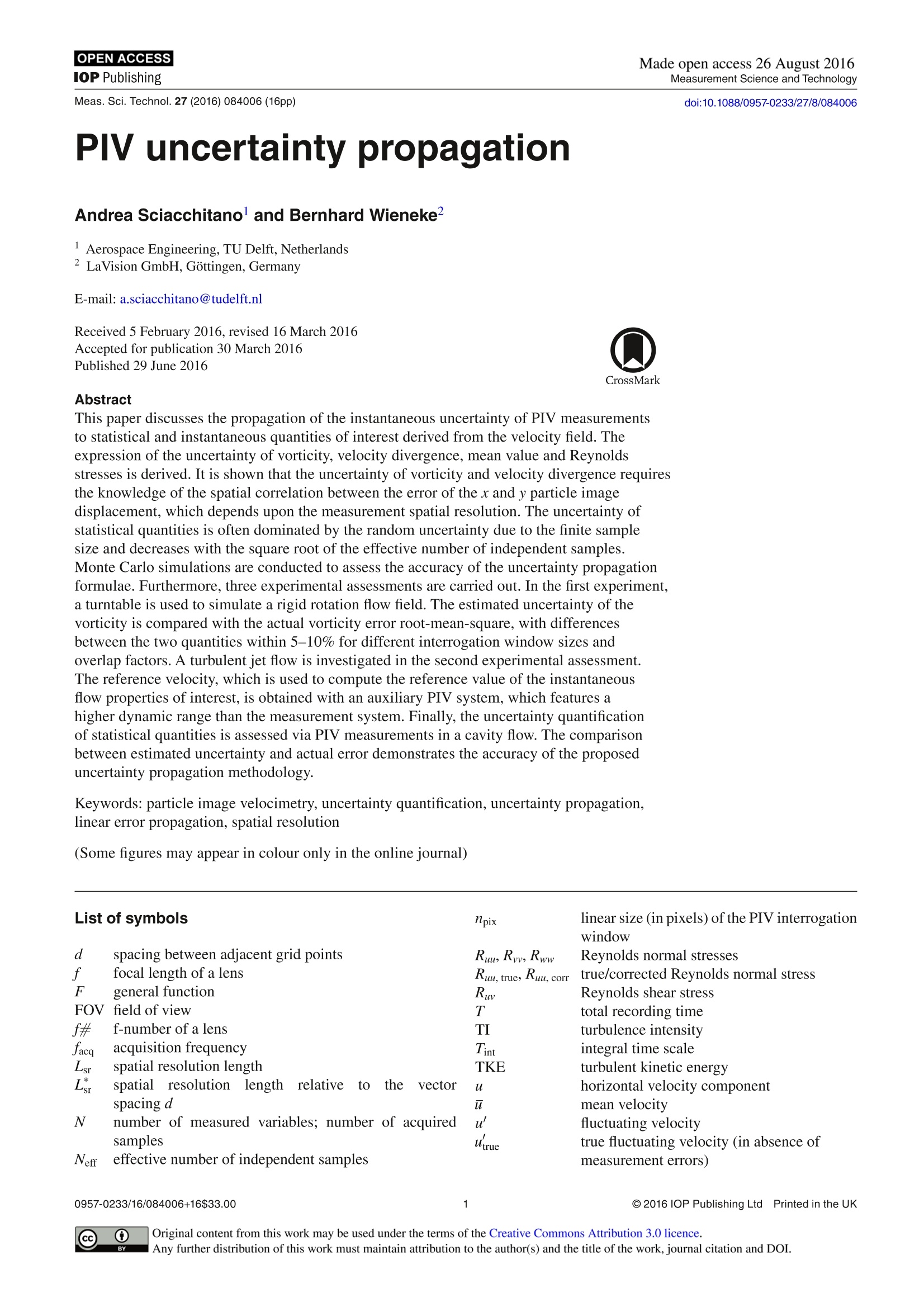
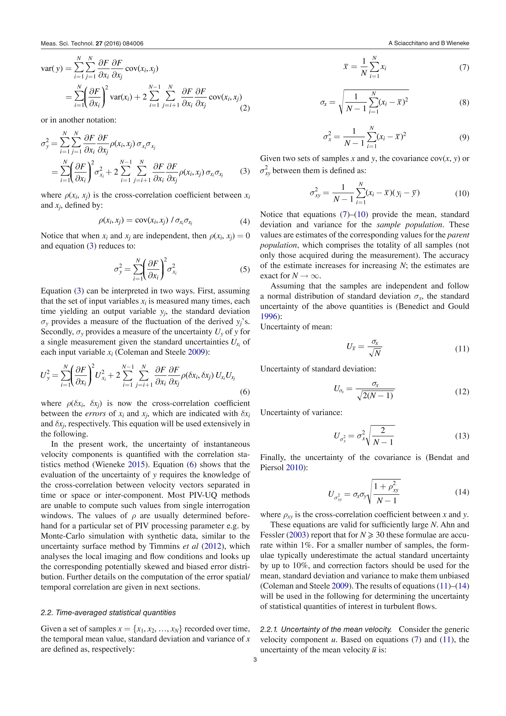
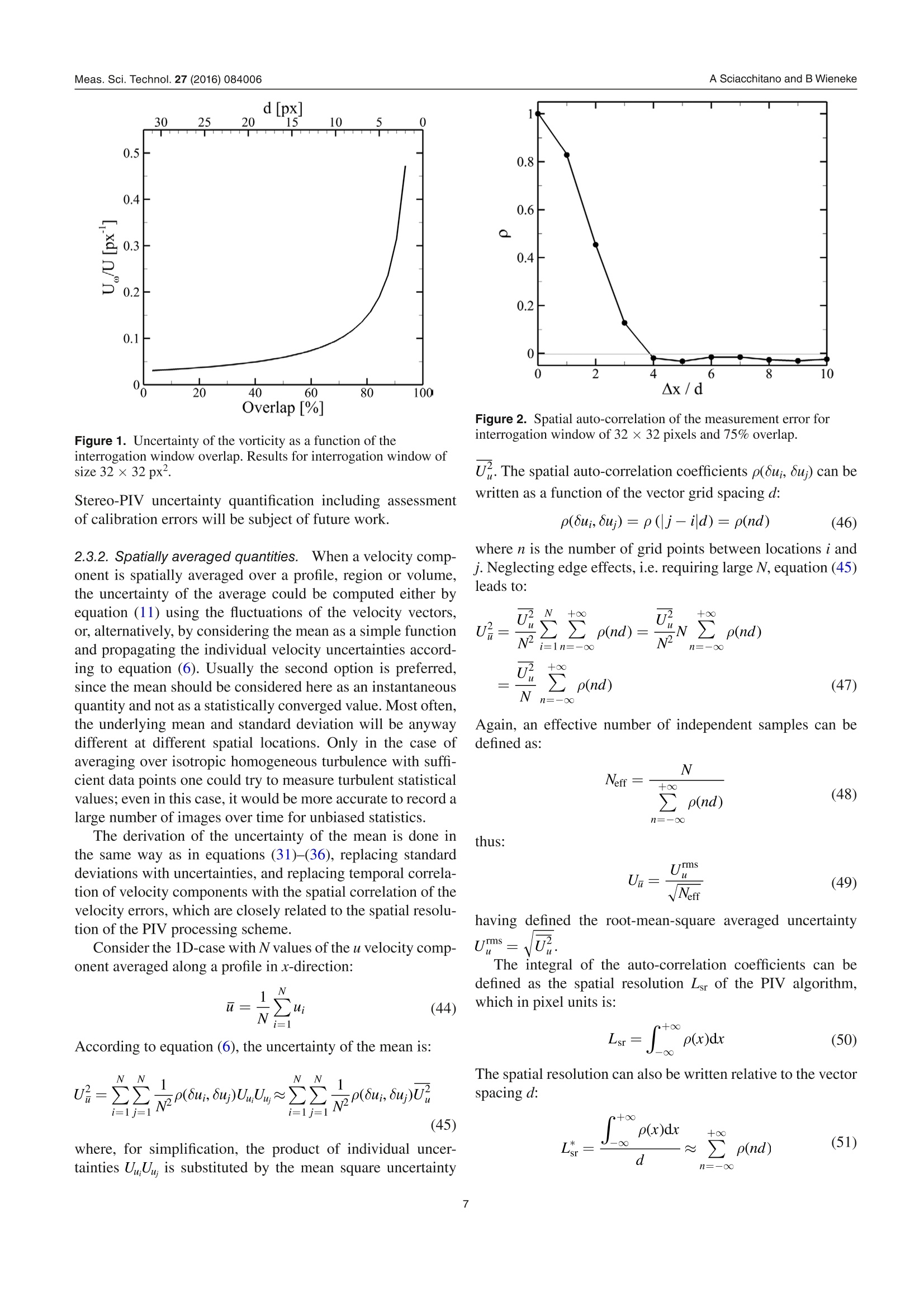
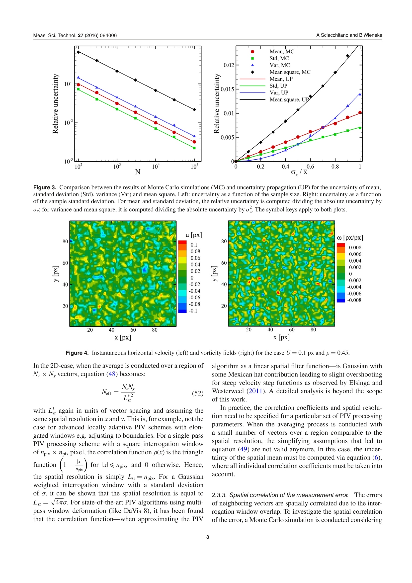
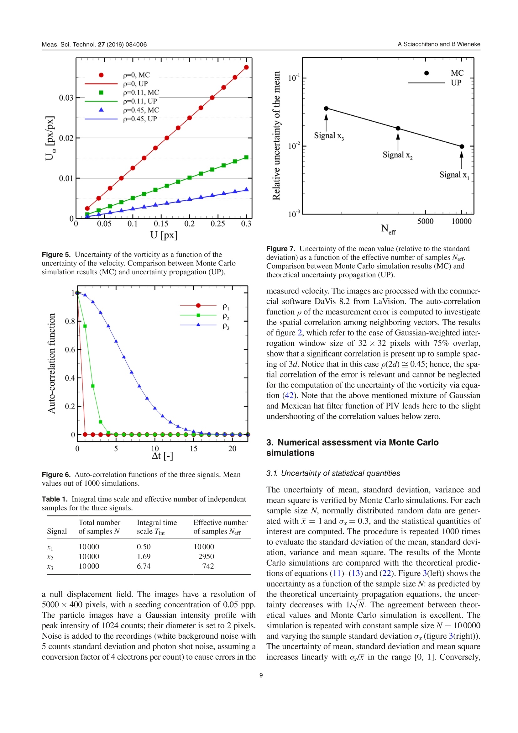
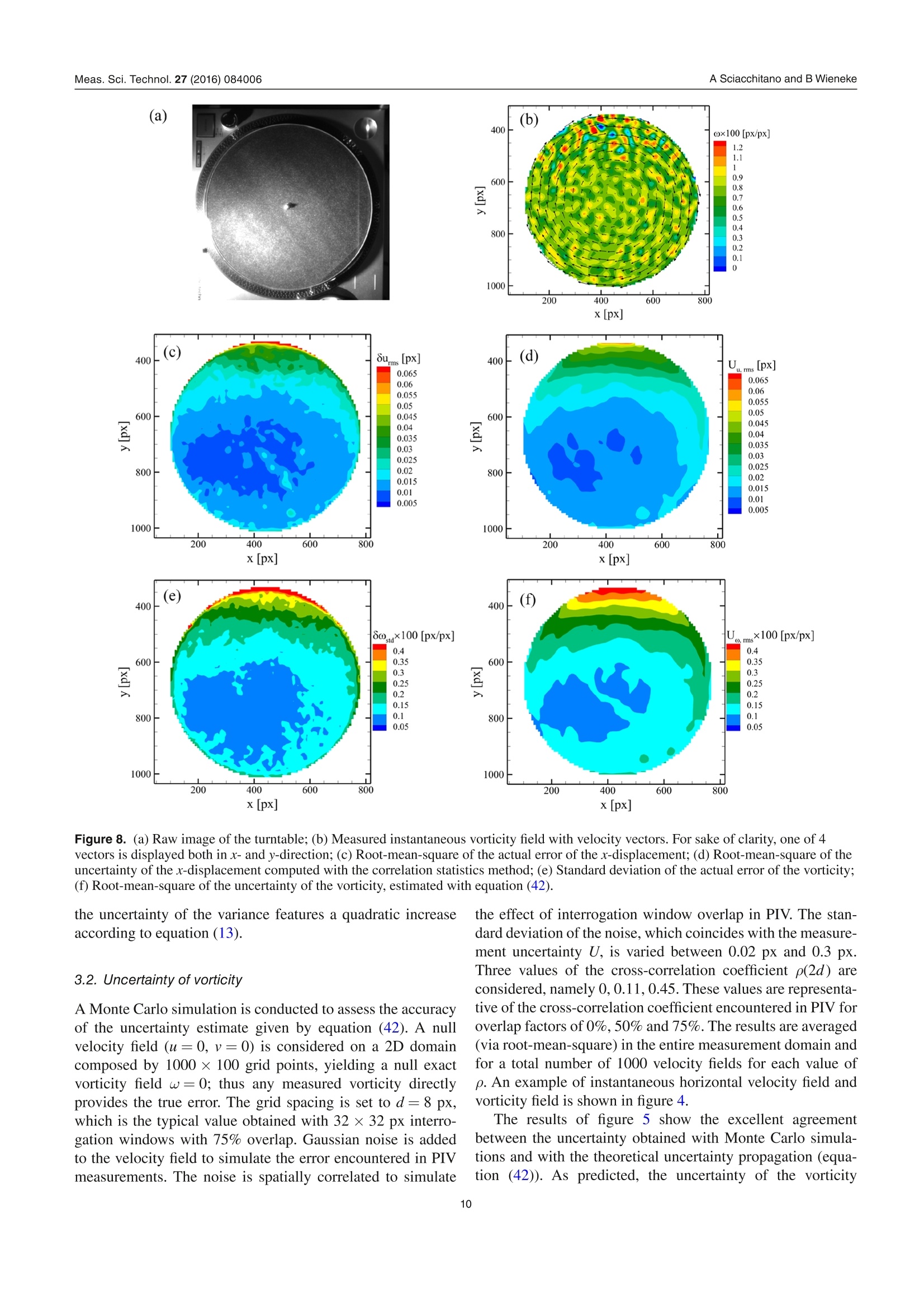
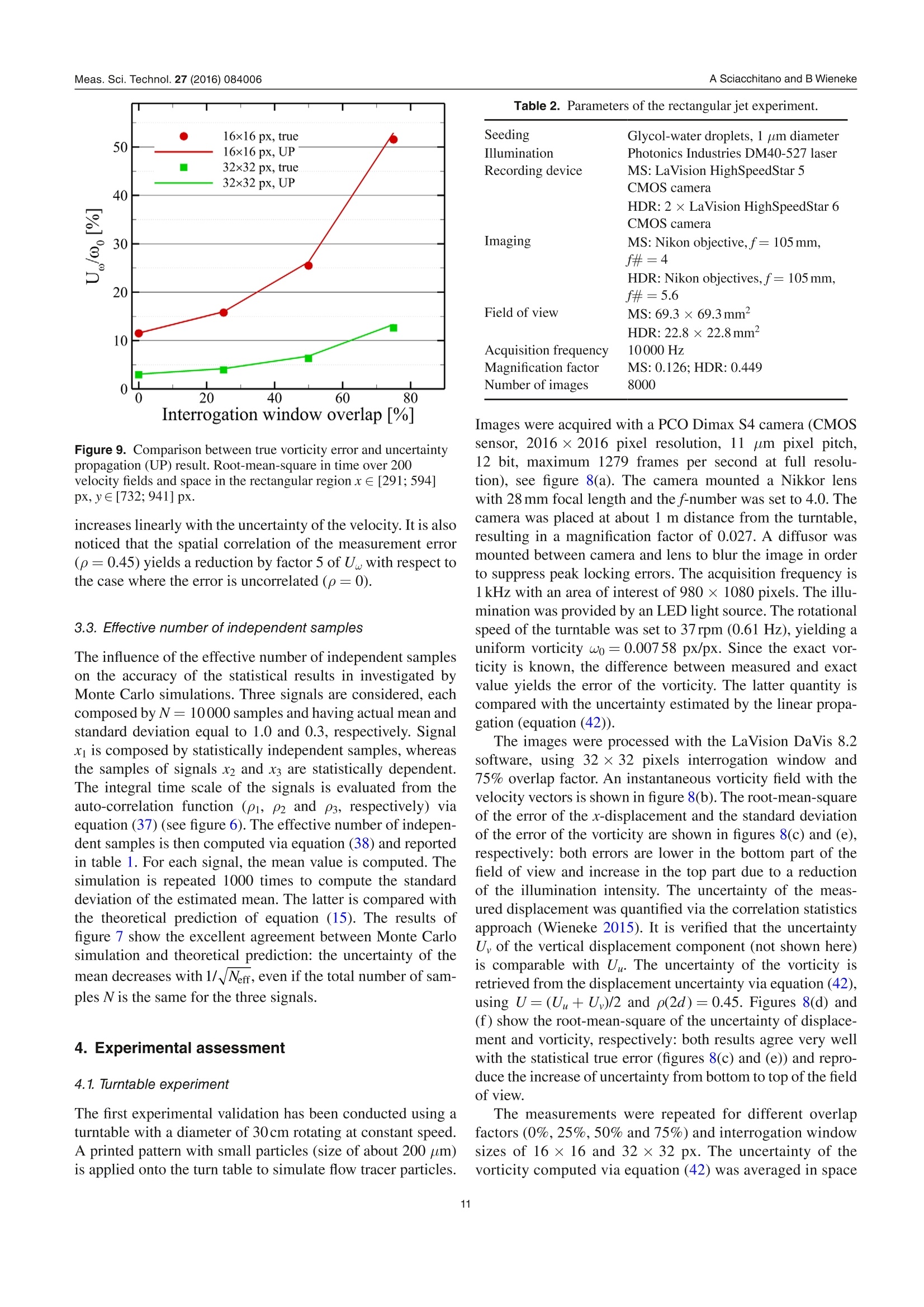
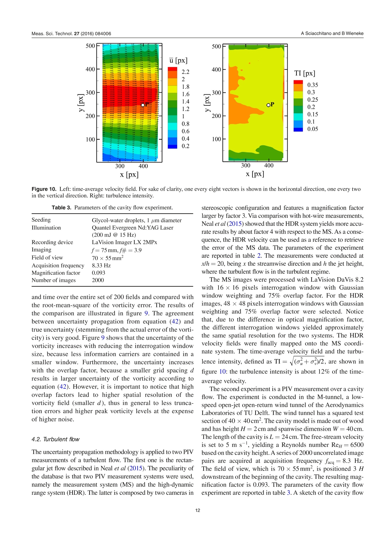
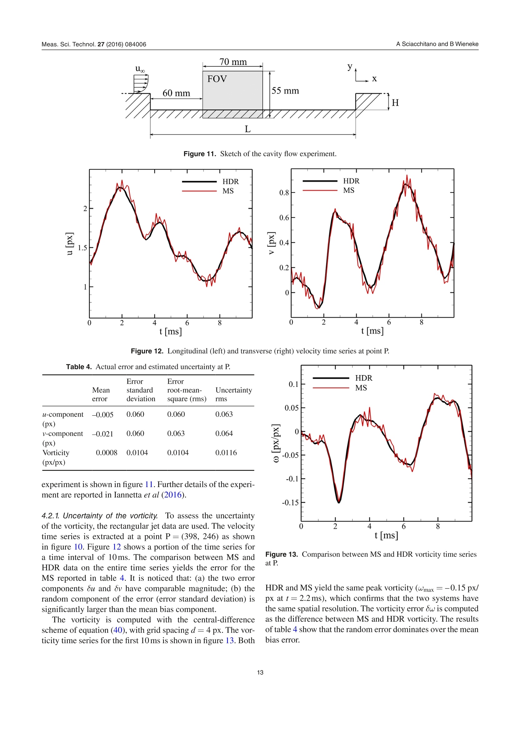
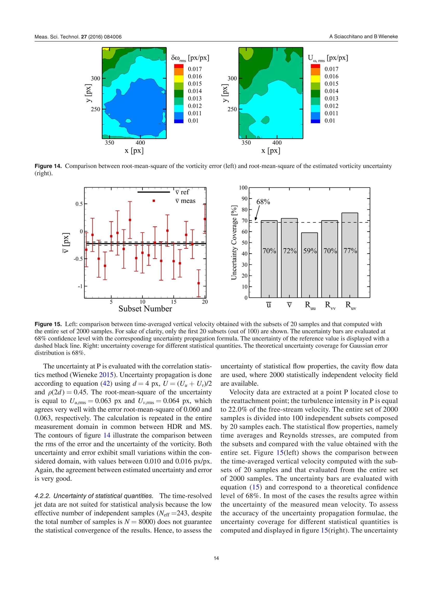
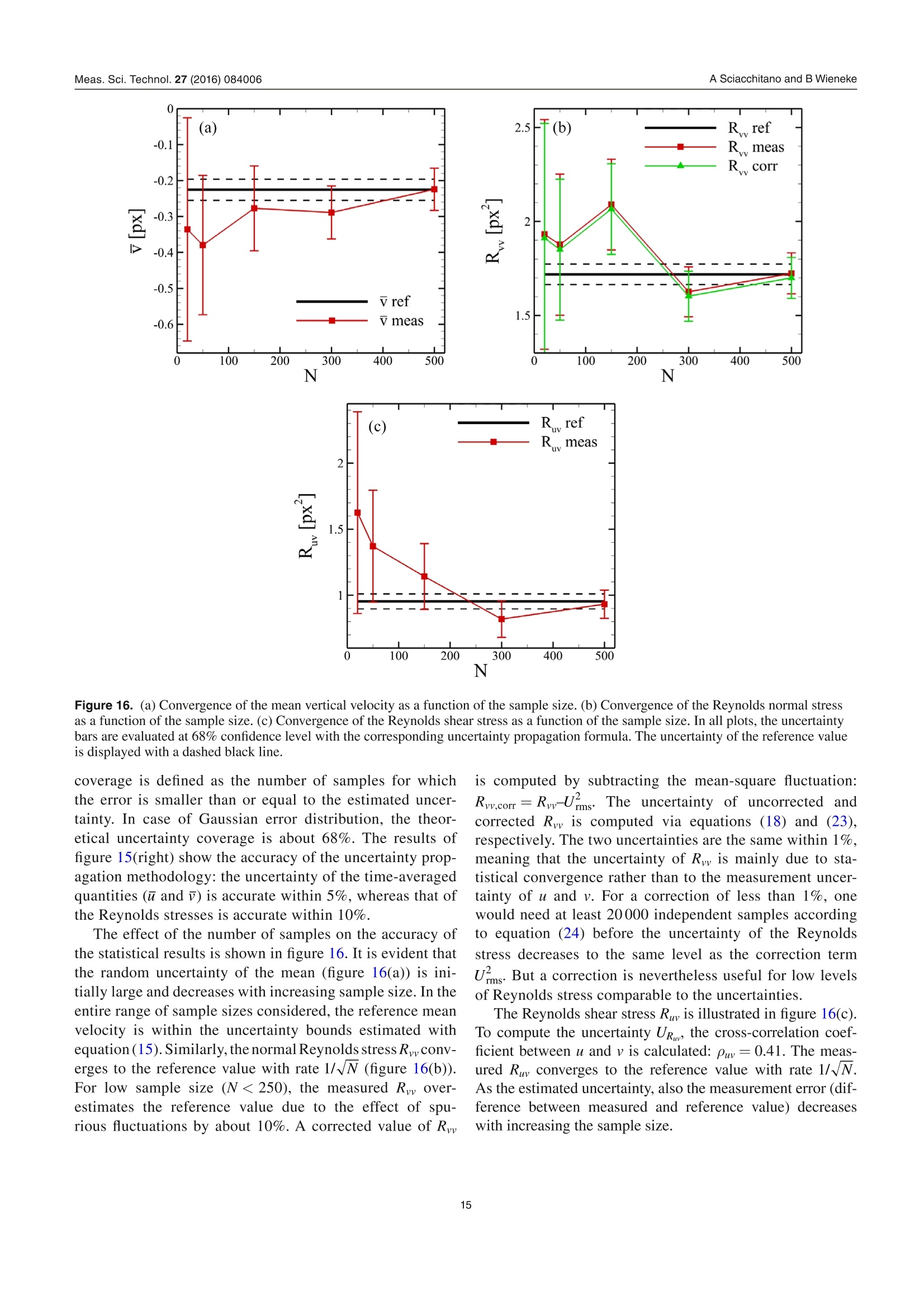
iopscience.iop.org OPEN ACCESSMade open access 26 August 2016Measurement Science and TechnologyIOP Publishing Home Search Collections Journals AbouttContact usMy lOPscience PIV uncertainty propagation This content has been downloaded from IOPscience. Please scroll down to see the full text.2016 Meas. Sci. Technol. 27 084006(http：//iopscience.iop.org/0957-0233/27/8/084006) View the table of contents for this issue， or go to the journal homepage for more Download details： |P Address： 219.143.130.209 This content was downloaded on 10/02/2017 at 02：52 Please note that terms and conditions apply. You may also be interested in： Collaborative framework for PIV uncertainty quantification： comparative assessment of methods Andrea Sciacchitano， Douglas R Neal， Barton L Smith et al. PIV uncertainty quantification from correlation statistics Bernhard Wieneke Collaborative framework for PlV uncertainty quantification： the experimental database Douglas R Neal， Andrea Sciacchitano， Barton L Smith et al. A comparative experimental evaluation of uncertainty estimation methods for two-component PIV Aaron Boomsma， Sayantan Bhattacharya， Dan Troolin et al. Application of a dual-plane particle image velocimetry technique L J Souverein， B W van Oudheusden， F Scarano et al. Stereo-particle image velocimetry uncertainty quantification Sayantan Bhattacharya， John J Charonko and Pavlos P Vlachos PIV uncertainty quantification by image matching Andrea Sciacchitano， Bernhard Wieneke and Fulvio Scarano Uncertainty on PIV mean and fluctuating velocity due to bias and random errors Brandon M Wilson and Barton L Smith Taylor-series and Monte-Carlo-method uncertainty estimation of the width of a probability distribution based on varying bias and random error Brandon M Wilson and Barton L Smith PlV uncertainty propagation Andrea Sciacchitano' and Bernhard Wieneke Aerospace Engineering， TU Delft， NetherlandsLaVision GmbH， Gottingen， Germany E-mail： a.sciacchitano@tudelft.nl Received 5 February 2016， revised 16 March 2016Accepted for publication 30 March 2016 Published 29 June 2016 Abstract This paper discusses the propagation of the instantaneous uncertainty of PIV measurementsto statistical and instantaneous quantities of interest derived from the velocity field. Theexpression of the uncertainty of vorticity， velocity divergence， mean value and Reynoldsstresses is derived. It is shown that the uncertainty of vorticity and velocity divergence requiresthe knowledge of the spatial correlation between the error of the x and y particle imagedisplacement， which depends upon the measurement spatial resolution. The uncertainty ofstatistical quantities is often dominated by the random uncertainty due to the finite samplesize and decreases with the square root of the effective number of independent samples.Monte Carlo simulations are conducted to assess the accuracy of the uncertainty propagationformulae. Furthermore， three experimental assessments are carried out. In the first experiment，a turntable is used to simulate a rigid rotation flow field. The estimated uncertainty of thevorticity is compared with the actual vorticity error root-mean-square， with differencesbetween the two quantities within 5-10% for different interrogation window sizes andoverlap factors. A turbulent jet flow is investigated in the second experimental assessment.The reference velocity， which is used to compute the reference value of the instantaneousflow properties of interest， is obtained with an auxiliary PIV system， which features ahigher dynamic range than the measurement system. Finally， the uncertainty quantificationof statistical quantities is assessed via PIV measurements in a cavity flow. The comparisonbetween estimated uncertainty and actual error demonstrates the accuracy of the proposeduncertainty propagation methodology. Keywords： particle image velocimetry，uncertainty quantification， uncertainty propagation，linear error propagation， spatial resolution (Some figures may appear in colour only in the online journal) List of symbolsnpix linear size (in pixels) of the PIV interrogationwindowdspacing between adjacent grid pointsRuuyRp， Rww Reynolds normal stressesffocal length of a lensRuu， true， Ruu， corrttrue/corrected Reynolds normal stressgeneral functionRuy Reynolds shear stressFOV ffield of viewTtotal recording timef-number of a lens t urbulence intensityacquisition frequency integral time scalespatial resolution lengthTKE turbulent kinetic energyspatial1 resolution 1lengthl Irelativeto the vectorhorizontal velocity componentspacing dmean velocityN number of measured variables； number of acquiredfluctuating velocitysamplesWtrue true fluctuating velocity (in absence ofNerr effective number of independent samplesmeasurement errors) 1. Introduction Uncertainty quantification in particle image velocimetry(PIV) is crucial to determine an interval that contains the mea-surement error. Several a-posteriori PIV uncertainty quantifi-cation methods have been recently proposed to estimate theunknown error for every velocity vector in the flow field. In the ‘uncertainty surface’method by Timmins et al(2012)， the recorded images are analyzed to quantify the mag-nitude of relevant error sources (particle image size，particledensity， displacements and shear). Comparing to previouslycomputed errors using synthetic data leads to uncertaintyestimation for every vector. The ‘peak ratio’ method byCharonko and Vlachos (2013) makes use of an empirical rela-tion between uncertainty and the ratio between the highest andthe second highest correlation peak. Further advances on thequantification of the measurement uncertainty based on thecross-correlation signal-to-noise ratio have been proposed byXue et al (2014). In the ‘image matching’or ‘particle dis-、、parity’ method by Sciacchitano et al (2013)， the measureddisplacement field is used to deform the recorded images，and the residual disparity in the position of matching particleimages leads to an estimate of the uncertainty of the displace-ment vector. Finally， the ‘correlation statistics’method byWieneke (2015) analyzes the contribution of all pixel intensi-ties to a possible asymmetry of the correlation peak， which isrelated to the uncertainty of the displacement vector. All thesemethods allow the a-posteriori quantification of the instanta-neous measurement uncertainty. A thorough comparison oftheir performances in different imaging and flow conditions is reported in Sciacchitano et al (2015)， where the dedicatedexperimental data from Neal et al (2015) is used. In many applications， PIV measurements are conductedto investigate flow properties derived from the velocity field，which can be instantaneous (e.g. vorticity， velocity diver-gence， acceleration， turbulence dissipation rate， pressure) orstatistical quantities (e.g. time average and Reynolds stresses).Therefore， once the uncertainties of the instantaneous velocitycomponents are estimated， they need to be propagated intothe derived quantities of interest. The quantification of theuncertainty of derived quantities relies upon the followingconsiderations： i. the uncertainty of the velocity components propagates tothat of the derived quantity of interest； ii. the correlation (in space， time and/or inter-component)of velocity components affects the uncertainty of derivedquantities； iii. for statistical quantities， additional uncertainty is dueto the finite number of samples N， which yields lack ofstatistical convergence. The works of Wilson and Smith (2013a，2013b) provideupper and lower uncertainty bounds for a number of statisticalquantities， such as average， variance and covariance. In theiranalysis， the authors considered the contributions of randomerrors， mainly due to the finite sample size， and unknowntime-dependent systematic errors. For velocity variance andcovariance， the lower uncertainty bound was found to belargerthan the upper uncertainty bound because spurious fluctua-tions tend to elevate the time-averaged measured fluctuations，yielding an error in the negative direction. In the work pre-sented here， uncertainty quantification is provided for manycommonly used derived quantities in PIV processing， bothstatistical and instantaneous. Following Coleman and Steele(2009)， we assume that each systematic error whose sign andmagnitude are known has been removed by correction. Thusthe paper focuses on random errors and uncertainties. Thework discusses the basic concepts of uncertainty propagationand its applications for flow properties of interest in typicalPIV measurements， such as vorticity， mean velocity andReynolds stresses. Furthermore， a correction of the Reynoldsstresses based on the magnitude of the noisy fluctuations isproposed. 2. Uncertainty propagation methodology 2.1. Basic concepts Let us consider a derived quantity of interest y， which is ageneral function F of N measured variables xi， with i=1，2，...，N. Assuming that each variable x； has a standard deviation ox，and given sufficient linearity of F， the variance of y can beapproximated by the variance-covariance matrix of F (Bendatand Piersol 2010)： or in another notation： where p(xi， x；) is the cross-correlation coefficient between x；and x， defined by： Notice that when x and xjare independent， then p(xi， Xj)= 0and equation (3) reduces to： Equation (3) can be interpreted in two ways. First， assumingthat the set of input variables x； is measured many times， eachtime yielding an output variable yj， the standard deviationay provides a measure of the fluctuation of the derived y’sSecondly， ay provides a measure of the uncertainty U， of y fora single measurement given the standard uncertainties Ux ofeach input variable x；(Coleman and Steele 2009)： (6) where p(8x， 6x；) is now the cross-correlation coefficientbetween the errors of x； andx；， which are indicated with ox；and oxj， respectively. This equation will be used extensively inthe following. In the present work， the uncertainty of instantaneousvelocity components is quantified with the correlation sta-tistics method (Wieneke 2015). Equation (6) shows that theevaluation of the uncertainty of yrequires the knowledge ofthe cross-correlation between velocity vectors separated intime or space or inter-component. Most PIV-UQmethodsare unable to compute such values from single interrogationwindows. The values of p are usually determined before-hand for a particular set of PIV processing parameter e.g. byMonte-Carlo simulation with synthetic data， similar to theuncertainty surface method by Timmins et al (2012)， whichanalyses the local imaging and flow conditions and looks upthe corresponding potentially skewed and biased error distri-bution. Further details on the computation of the error spatial/temporal correlation are given in next sections. 2.2. Time-averaged statistical quantities Given a set of samples x={x1，X2，…..，xN} recorded over time，the temporal mean value， standard deviation and variance of xare defined as， respectively： Given two sets of samples x and y， the covariance cov(x， y) orbetween them is defined as： Notice that equations (7)-(10) provide the mean， standarddeviation and variance for the sample population. Thesevalues are estimates of the corresponding values for the parentpopulation， which comprises the totality of all samples (notonly those acquired during the measurement). The accuracyof the estimate increases for increasing N； the estimates areexact for N→o. Assuming that the samples are independent and followa normal distribution of standard deviation ax， the standarduncertainty of the above quantities is (Benedict and Gould1996)： Uncertainty of mean： Uncertainty of standard deviation： Uncertainty of variance： Finally， the uncertainty of the covariance is (Bendat andPiersol 2010)： where pxy is the cross-correlation coefficient between x and y. . These equations are valid for sufficiently large N. Ahn andFessler (2003) report that for N≥30 these formulae are accu-rate within 1%. For a smaller number of samples， the form-ulae typically underestimate the actual standard uncertaintyby up to 10%， and correction factors should be used for themean， standard deviation and variance to make them unbiased(Coleman and Steele 2009). The results of equations (11)-(14)will be used in the following for determining the uncertaintyof statistical quantities of interest in turbulent flows. 2.2.1. Uncertainty of the mean velocity. Consider the genericvelocity component u. Based on equations (7) and (11)， theuncertainty of the mean velocity u is： Analogous equations are obtained for the v and w velocitycomponents. In equation (15)， systematic uncertainties due tospatial modulation errors or peak locking are not taken intoaccount. The standard deviation ou contains both the truevelocity fluctuations (ou， fluct) and the measurement errors(ouerr)： where Uu is the uncertainty of the instantaneous velocitycomponent and U- is the mean-square of U. The right-hand-side of equation (16) is obtained by considering that the errorvariance ouer is approximately equal to the uncertainty mean-square U for accurate uncertainty quantification methods(see appendix of Sciacchitano et al 2015). When the samples are not independent， the parameter N ofequation (15) must be substituted with the effective number ofindependent samples Neff， as discussed in section 2.2.3. 2.2.2. Uncertainty of Reynolds stress. The Reynolds stressplays a crucial role in turbulent flows because it representsthe rate of mean momentum transfer by turbulent fluctuations.In this section， the expression of the uncertainty is derived forthe Reynolds normal stress and for the Reynolds shear stress. Reynolds normal stress. The Reynolds normal stress for thex-velocity component u is defined as the variance of u： where u'is the fluctuating part of u： u'=u- u. Due to its def-inition， the uncertainty of Ruu is computed with equation (13)： It is assumed that the samples are statistically independent.If not， N must again be substituted with the effective numberof independent samples Neff (section 2.2.3). As discussed insection 2.2.1， ou contains both the effects of true velocity fluc-tuations and spurious fluctuations due to noise. The latter yieldan over-estimate for Ruu with respect to the true value Ruu，true： When the uncertainty of the measured velocity is known，a corrected (more accurate) estimate of Ruu can be retrieved bysubtracting the spurious fluctuations mean square Ufrom themeasured Reynolds stress： Thus， according to equation (6)， the uncertainty of the cor-rected normal Reynolds stress estimate Ruu， corr， indicated withURm.cor is given by： The latter is composed by two components：(a) the uncer-tainty of the measured Reynolds stress， which is given byequation(18)； (b) the uncertainty of the spurious fluctuationsmean square U. Notice that U can only assume positivevalues， therefore its distribution is better approximated by alog-normal distribution rather than by a Gaussian distribution.At least when approximating the distribution with a Gaussiandistribution with positive mean， an analytical expression ofthe uncertainty of U can be derived using equation (6)： The accuracy of equation (22) is assessed in section 3.1.Combining both equations (18) and (22)， the uncertainty ofRuu， corr is： In many applications， the measurement error is small withrespect to the actual velocity fluctuations， therefore the termwithin brackets is negligible and equation (23) reduces to： In practice， the uncertainty of the Reynolds normal stressaccording to (23) and (24) is often strongly underestimatedfor two reasons. First， the subtraction of equation (20) is sub-ject to the accuracy of the uncertainty quantification methoditself. As shown by Sciacchitano et al (2015)， the uncertaintyestimations of state-of-the-art UQ methods may deviate fromthe true errors by as much as a factor two for different flowand imaging conditions. Secondly， the finite spatial resolutionof the PIV processing algorithm does not allow resolving fluc-tuations of length scale smaller than about the interrogationwindow. This may lead to a substantial underestimation of Ruudepending on Reynolds number， turbulent level and imagingmagnification. It is important to remark here that the computation of theuncertainty of Ruu according to equation (18) does not require theknowledge of the uncertainty of the instantaneous velocity. Onthe other hand， in order to compute the corrected value Ruu，corr，the uncertainty of the instantaneous velocity must be known. Turbulent kinetic energyV.The turbulent kinetic energy TKEis defined as half of the sum of the Reynolds normal stresses： Based on the error propagation formula (6)， the uncertainty ofthe TKE is equal to： Assuming N > 1 and that the instantaneous measurementuncertainty is negligible with respect to the velocity fluctua-tions， the result of equation (24) can be used and the expres-sion of UTKE reduces to： When Rww is unknown (e.g. in planar PIV， which only pro-vides two velocity components)， its value can be estimatedas Rww=(Ruu+R)/2 under the assumption of isotropicturbulence. Reynolds shear stress.The Reynolds shear stress Ruy isdefined as the covariance of the u and v velocity components： The quantity puy is the cross-correlation coefficient betweenthe velocity components u and v. Assuming that the velocityfluctuations are affected by error ou and ov， respectively， andthat the error of the time-averaged velocity is negligible， equa-tion (28) becomes： In equation (29)， Pouoy is the cross-correlation coefficientbetween the errors of the two velocity components. Thetrue velocity fluctuations are assumed to be independent ofthe measurement errors， thus cancelling the cross-terms(u，trueov) and =(trueou). As a consequence， theReynolds shear stress Ruy exhibits a systematic error (equal to PnovUU) only if Su and Sv are correlated (Pbuby =0)；however， this is typically not the case for planar 2 C-PIV.Conversely， for stereo-PIV there may be non-zero inter-component correlations dependent on the experimental setupof the two cameras relative to the x- and y-axis. The uncer-tainty of Ruy is obtained by applying the covariance uncer-tainty equation (14)： The uncertainty of the Reynolds shear stress has a minimumvalue of ouo/√N-1when u and v are uncorrelated and increases with higher correlation between the two velocitycomponents. 2.2.3. Effective number of independent samples. Consider ageneric statistical quantity， as the mean x. In this section wewill show that if the N samples from which x is computed arenot independent， a larger uncertainty of x is expected. In fact，from equation (6) it is obtained： having assumed a constant underlying fluctuation distributionox=0x=C. The auto-correlation coefficient p(xi， x；) can bewritten as： with At the inverse of the sampling frequency. The auto-correlation coefficient p is a function of the time separationn▲t between samples xi and x；=Xi+n. As a result， equa-tion (31) can be written as： The quantity p(nAt) is equal to one for n =0 and decays tozero for increasing n. Furthermore， p(n▲t) is an even func-tion： p(n▲t)= p(-n▲t). Assuming N→ o and neglecting theedge effects in the summation， equation (33) becomes： Defining the effective number of independent samples as： leads to： Typically， the summation of equation (35) is stopped when thecorrelation value reaches zero for the first time. Notice thatwhen the samples are uncorrelated，then p(n▲t) is 1 for n=0and zero otherwise， so in this case Nerf =N. Conversely， whenthe samples are correlated then p(n▲t)> 1； thereforeNerr is smaller than N， thus the uncertainty of the mean valueis larger. The integral time scale Tint is defined as the integral of theauto-correlation function p(t) of the time series x(t) (Georgeet al 1978)： Tint is a measure of the time interval over which x(t) is depen-dent on itself. For time intervals large compared to Tint， x(t)becomes statistically independent of itself. Then， the effectivenumber of independent samples can be written as a functionof the observation time T and the integral time scale Tint： The relevance of equations (36) and (38) for experimentalmeasurements in turbulent flows is discussed by Tennekesand Lumley (1972) among others. The equations illustratethe fact that， when ▲t -0.02 -0.04 -0.006 -0.06 -0.008 -0.08 -0.1 x[px] x[px] In the 2D-case， when the average is conducted over a region ofNx× N， vectors， equation (48) becomes： with Lsr again in units of vector spacing and assuming thesame spatial resolution in x and y. This is， for example， not thecase for advanced locally adaptive PIV schemes with elon-gated windows e.g. adjusting to boundaries. For a single-passPIV processing scheme with a square interrogation windowof npix× npix pixel， the correlation function p(x) is the trianglefunction() ffoor rlxl≤npix， and 0 otherwise. Hence，the spatial resolution is simply Lsr= npix. For a Gaussianweighted interrogation window with a standard deviationof o， it can be shown that the spatial resolution is equal toLsr =√4no. For state-of-the-art PIV algorithms using multi-pass window deformation (like DaVis 8)， it has been foundthat the correlation function-when approximating the PIV algorithm as a linear spatial filter function-is Gaussian withsome Mexican hat contribution leading to slight overshootingfor steep velocity step functions as observed by Elsinga andWesterweel (2011). A detailed analysis is beyond the scopeof this work. In practice， the correlation coefficients and spatial resolu-tion need to be specified for a particular set of PIV processingparameters. When the averaging process is conducted witha small number ofvectors over a region comparable to thespatial resolution， the simplifying assumptions that led toequation (49) are not valid anymore. In this case， the uncer-tainty of the spatial mean must be computed via equation (6)，where all individual correlation coefficients must be taken intoaccount. 2.3.3. Spatial correlation of the measurement error.TThe errorsof neighboring vectors are spatially correlated due to the inter-rogation window overlap. To investigate the spatial correlationof the error， a Monte Carlo simulation is conducted considering Figure 5. Uncertainty of the vorticity as a function of theuncertainty of the velocity. Comparison between Monte Carlosimulation results (MC) and uncertainty propagation (UP). Figure 6. Auto-correlation functions of the three signals. Meanvalues out of 1000 simulations. Table 1. Integral time scale and effective number of independentsamples for the three signals. Total number Integral time Effective number Signal of samples N scale Tint of samples Neff X1 10000 0.50 10000 X2 10000 1.69 2950 X3 10000 6.74 742 a null displacement field. The images have a resolution of5000 ×400 pixels， with a seeding concentration of 0.05 ppp.The particle images have a Gaussian intensity profile withpeak intensity of 1024 counts； their diameter is set to 2 pixels.Noise is added to the recordings (white background noise with5 counts standard deviation and photon shot noise， assuming aconversion factor of 4 electrons per count) to cause errors in the Figure 7. Uncertainty of the mean value (relative to the standarddeviation) as a function of the effective number of samples Neff.Comparison between Monte Carlo simulation results (MC) andtheoretical uncertainty propagation (UP). measured velocity. The images are processed with the commer-cial software DaVis 8.2 from LaVision. The auto-correlationfunction p of the measurement error is computed to investigatethe spatial correlation among neighboring vectors. The resultsof figure 2， which refer to the case of Gaussian-weighted inter-rogation window size of 32×32 pixels with 75% overlap，show that a significant correlation is present up to sample spac-ing of 3d. Notice that in this case p(2d)=0.45； hence， the spa-tial correlation of the error is relevant and cannot be neglectedfor the computation of the uncertainty of the vorticity via equa-tion (4). Note that the above mentioned mixture of Gaussianand Mexican hat filter function of PIV leads here to the slightundershooting of the correlation values below zero. 3. Numerical assessment via Monte Carlosimulations 3.1. Uncertainty of statistical quantities The uncertainty of mean， standard deviation， variance andmean square is verified by Monte Carlo simulations. For eachsample size N， normally distributed random data are gener-ated with x= 1 and ox=0.3， and the statistical quantities ofinterest are computed. The procedure is repeated 1000 timesto evaluate the standard deviation of the mean， standard devi-ation， variance and mean square. The results of the MonteCarlo simulations are compared with the theoretical predic-tions of equations (11)-(13) and (22). Figure 3(left) shows theuncertainty as a function of the sample size N： as predicted bythe theoretical uncertainty propagation equations， the uncer-tainty decreases with 1/√N. The agreement between theor-etical values and Monte Carlo simulation is excellent. Thesimulation is repeated with constant sample size N=100000and varying the sample standard deviation ox (figure 3(right)).The uncertainty of mean， standard deviation and mean squareincreases linearly with or/x in the range [0， 1]. Conversely， 0.065 0.06 0.055 0.05 0.045 0.04 0.035 0.03 0.025 0.02 0.015 0.01 0.005 80 ×100 [px/px] x [px] Figure 8. (a)Raw image of the turntable； (b) Measured instantaneous vorticity field with velocity vectors. For sake of clarity， one of 4vectors is displayed both in x- and y-direction； (c) Root-mean-square of the actual error of the x-displacement； (d) Root-mean-square of theuncertainty of the x-displacement computed with the correlation statistics method； (e) Standard deviation of the actual error of the vorticity；(f) Root-mean-square of the uncertainty of the vorticity， estimated with equation(42). 3.2.Uncertainty of vorticity A Monte Carlo simulation is conducted to assess the accuracyof the uncertainty estimate given by equation (42). A nullvelocity field (u=0， v=0) is considered on a 2D domaincomposed by 1000 × 100 grid points， yielding a null exactvorticity field w=0； thus any measured vorticity directlyprovides the true error. The grid spacing is set to d=8 px，which is the typical value obtained with 32×32 px interro-gation windows with 75% overlap. Gaussian noise is addedto the velocity field to simulate the error encountered in PIVmeasurements. The noise is spatially correlated to simulate the effect of interrogation window overlap in PIV. The stan-dard deviation of the noise， which coincides with the measure-ment uncertainty U， is varied between 0.02 px and 0.3 px.Three values of the cross-correlation coefficient p(2d) areconsidered， namely 0， 0.11， 0.45. These values are representa-tive of the cross-correlation coefficient encountered in PIV foroverlap factors of 0%， 50% and 75%. The results are averaged(via root-mean-square) in the entire measurement domain andfor a total number of 1000 velocity fields for each value ofp. An example of instantaneous horizontal velocity field andvorticity field is shown in figure 4. The results of figure 5 show the excellent agreementbetween the uncertainty obtained with Monte Carlo simula-tions and with the theoretical uncertainty propagation (equa-tion (42)). As predicted， the uncertainty of the vorticity Figure 9. Comparison between true vorticity error and uncertaintypropagation (UP) result.Root-mean-square in time over 200velocity fields and space in the rectangular region x E [291；594]px，yE[732；941] px. increases linearly with the uncertainty of the velocity. It is alsonoticed that the spatial correlation of the measurement error(p=0.45) yields a reduction by factor 5 of U with respect tothe case where the error is uncorrelated (p=0). 3.3. Effective number of independent samples The influence of the effective number of independent sampleson the accuracy of the statistical results in investigated byMonte Carlo simulations. Three signals are considered，eachcomposedby N=10000 samples and having actual mean andstandard deviation equal to 1.0 and 0.3， respectively. Signalxis composed by statistically independent samples， whereasthe samples of signals x2 and x3 are statistically dependent.The integral time scale of the signals is evaluated from theauto-correlation function (P1， P2 and p3， respectively) viaequation (37) (see figure6). The effective number of indepen-dent samples is then computed via equation (38) and reportedin table 1. For each signal， the mean value is computed. Thesimulation is repeated 1000 times to compute the standarddeviation of the estimated mean. The latter is compared withthe theoretical prediction of equation (15). The results offigure 7 show the excellent agreement between Monte Carlosimulation and theoretical prediction： the uncertainty of themean decreases with 1/√Neff， even if the total number of sam-ples N is the same for the three signals. 4. Experimental assessment 4.1. Turntable experiment The first experimental validation has been conducted using aturntable with a diameter of 30 cm rotating at constant speed.A printed pattern with small particles (size of about 200 um)is applied onto the turn table to simulate flow tracer particles. Seeding Glycol-water droplets， 1 um diameter Illumination Photonics Industries DM40-527 laser Recording device MS： LaVision HighSpeedStar 5 CMOS camera Imaging HDR： 2× LaVision HighSpeedStar 6 CMOS camera MS： Nikon objective，f=105mm， f#=4 HDR： Nikon objectives， f= 105mm， f#=5.6 Field of view MS： 69.3×69.3mm HDR：22.8×22.8mm Acquisition frequency 10000 Hz Magnification factor MS： 0.126； HDR： 0.449 Number of images 8000 Images were acquired with a PCO Dimax S4 camera (CMOSsensor， 2016×2016 pixel resolution， 11 um pixel pitch，12 bit， maximum 1279 frames per second at full resolu-tion)， see figure 8(a). The camera mounted a Nikkor lenswith 28 mm focal length and the f-number was set to 4.0. Thecamera was placed at about 1 m distance from the turntable，resulting in a magnification factor of 0.027. A diffusor wasmounted between camera and lens to blur the image in orderto suppress peak locking errors. The acquisition frequency is1kHz with an area of interest of 980×1080 pixels. The illu-mination was provided by an LED light source. The rotationalspeed of the turntable was set to 37rpm (0.61 Hz)， yielding auniform vorticity wo=0.00758 px/px. Since the exact vor-ticity is known， the difference between measured and exactvalue yields the error of the vorticity. The latter quantity iscompared with the uncertainty estimated by the linear propa-gation (equation(42)). The images were processed with the LaVision DaVis 8.2software， using 32 ×32 pixels interrogation window and75% overlap factor. An instantaneous vorticity field with thevelocity vectors is shown in figure 8(b). The root-mean-squareof the error of the x-displacement and the standard deviationof the error of the vorticity are shown in figures 8(c) and (e)，respectively： both errors are lower in the bottom part of thefield of view and increase in the top part due to a reductionof the illumination intensity. The uncertainty of the meas-ured displacement was quantified via the correlation statisticsapproach (Wieneke 2015). It is verified that the uncertaintyU， of the vertical displacement component (not shown here)is comparable with Uu. The uncertainty of the vorticity isretrieved from the displacement uncertainty via equation (42)，using U=(Uu+U，)/2 and p(2d)=0.45. Figures 8(d) and(f) show the root-mean-square of the uncertainty of displace-ment and vorticity， respectively： both results agree very wellwith the statistical true error (figures 8(c) and (e)) and repro-duce the increase of uncertainty from bottom to top of the fieldof view. The measurements were repeated for different overlapfactors (0%，25%，50% and 75%) and interrogation windowsizes of 16 × 16 and 32 × 32 px. The uncertainty of thevorticity computed via equation (42) was averaged in space Figure 10. Left： time-average velocity field. For sake of clarity， one every eight vectors is shown in the horizontal direction， one every twoin the vertical direction. Right： turbulence intensity. Table 3. Parameters of the cavity flow experiment. Seeding Glycol-water droplets， 1 um diameter Illumination Quantel Evergreen Nd：YAG Laser (200 mJ @ 15 Hz) Recording device LaVision Imager LX2MPx Imaging f= 75mm，f#=3.9 Field of view 70 ×55mm Acquisition frequency 8.33 Hz Magnification factor 0.093 Number of images 2000 and time over the entire set of 200 fields and compared withthe root-mean-square of the vorticity error. The results ofthe comparison are illustrated in figure 9. The agreementbetween uncertainty propagation from equation (42) andtrue uncertainty (stemming from the actual error of thevorti-city) is very good. Figure 9 shows that the uncertainty of thevorticity increases with reducing the interrogation windowsize， because less information carriers are contained in asmaller window. Furthermore， the uncertainty increaseswith the overlap factor， because a smaller grid spacing dresults in larger uncertainty of the vorticity according toequation (42). However， it is important to notice that highoverlap factors lead to higher spatial resolution of thevorticity field (smaller d)， thus in general to less trunca-tion errors and higher peak vorticity levels at the expenseof higher noise. 4.2. Turbulent flow The uncertainty propagation methodology is applied to two PIVmeasurements of a turbulent flow. The first one is the rectan-gular jet flow described in Neal et al (2015). The peculiarity ofthe database is that two PIV measurement systems were used，namely the measurement system (MS) and the high-dynamicrange system (HDR).The latter is composed by two cameras in stereoscopic configuration and features a magnification factorlarger by factor 3. Via comparison with hot-wire measurements，Neal et al(2015) showed that the HDR system yields more accu-rate results by about factor 4 with respect to the MS. As a conse-quence， the HDR velocity can be used as a reference to retrievethe error of the MS data. The parameters of the experimentare reported in table 2. The measurements were conducted atx/h=20， being x the streamwise direction and h the jet height，where the turbulent flow is in the turbulent regime. The MS images were processed with LaVision DaVis 8.2with 16× 16 pixels interrogation window with Gaussianwindow weighting and 75% overlap factor. For the HDRimages， 48 × 48 pixels interrogation windows with Gaussianweighting and 75% overlap factor were selected. Noticethat， due to the difference in optical magnification factor，the different interrogation windows yielded approximatelythe same spatial resolution for the two systems. The HDRvelocity fields were finally mapped onto the MS coordi-nate system. The time-average velocity field and the turbu-lence intensity， defined as TI=(o+)/2， are shown infigure 10： the turbulence intensity is about 12% of the time-average velocity. The second experiment is a PIV measurement over a cavityflow. The experiment is conducted in the M-tunnel， a low-speed open-jet open-return wind tunnel of the AerodynamicsLaboratories of TU Delft. The wind tunnel has a squared testsection of 40 x40cm. The cavity model is made out of woodand has height H=2 cm and spanwise dimension W= 40cm.The length of the cavity is L=24 cm. The free-stream velocityis set to 5 m s-，yielding a Reynolds number ReH=6500based on the cavity height. A series of 2000 uncorrelated imagepairs are acquired at acquisition frequency facq=8.3 Hz.The field of view， which is 70 ×55 mm， is positioned 3 Hdownstream of the beginning of the cavity. The resulting mag-nification factor is 0.093. The parameters of the cavity flowexperiment are reported in table 3. A sketch of the cavity flow Figure 11. Sketch of the cavity flow experiment. tms Figure 12. Longitudinal (left) and transverse (right) velocity time series at point P. Table 4. Actual error and estimated uncertainty at P. Error Error Mean standard root-mean- Uncertainty error deviation square (rms) rms u-component -0.005 0.060 0.060 0.063 (px) v-component -0.021 0.060 0.063 0.064 (px) Vorticity 0.0008 0.0104 0.0104 0.0116 (px/px) experiment is shown in figure 11. Further details of the experi-ment are reported in Iannetta et al (2016). 4.2.1. Uncertainty of the vorticity.To assess the uncertaintyof the vorticity， the rectangular jet data are used. The velocitytime series is extracted at a point P=(398， 246) as shownin figure 10. Figure 12 shows a portion of the time series fora time interval of 10ms. The comparison between MS andHDR data on the entire time series yields the error for theMS reported in table 4. It is noticed that： (a) the two errorcomponents ou and v have comparable magnitude； (b) therandom component of the error (error standard deviation) issignificantly larger than the mean bias component. The vorticity is computed with the central-differencescheme of equation (40)， with grid spacing d=4px.The vor-ticity time series for the first 10 ms is shown in figure 13. Both Figure 13. Comparison between MS and HDR vorticity time seriesat P. HDR and MS yield the same peak vorticity (wmax =-0.15 px/px at t=2.2 ms)， which confirms that the two systems havethe same spatial resolution. The vorticity error ow is computedas the difference between MS and HDR vorticity.The resultsoftable 4 show that the random error dominates over the meanbias error. Figure 14. Comparison between root-mean-square of the vorticity error (left) and root-mean-square of the estimated vorticity uncertainty(right). Figure 15. Left： comparison between time-averaged vertical velocity obtained with the subsets of 20 samples and that computed withthe entire set of 2000 samples. For sake of clarity， only the first 20 subsets (out of 100) are shown. The uncertainty bars are evaluated at68% confidence level with the corresponding uncertainty propagation formula. The uncertainty of the reference value is displayed with adashed black line. Right： uncertainty coverage for different statistical quantities. The theoretical uncertainty coverage for Gaussian errordistribution is 68%. The uncertainty at P is evaluated with the correlation statis-tics method (Wieneke 2015). Uncertainty propagation is doneaccording to equation (42) using d=4 px，U=(Uu+U)/2and p(2d)=0.45. The root-mean-square of the uncertaintyis equal to Uu，rms =0.063 px and Uv，rms=0.064 px， whichagrees very well with the error root-mean-square of 0.060 and0.063， respectively. The calculation is repeated in the entiremeasurement domain in common between HDR and MS.The contours of figure 14 illustrate the comparison betweenthe rms of the error and the uncertainty of the vorticity. Bothuncertainty and error exhibit small variations within the con-sidered domain， with values between 0.010 and 0.016 px/px.Again， the agreement between estimated uncertainty and erroris very good. 4.2.2. Uncertainty of statistical quantities.TThe time-resolvedjet data are not suited for statistical analysis because the loweffective number of independent samples (Neff =243， despitethe total number of samples is N=8000) does not guaranteethe statistical convergence of the results. Hence， to assess the uncertainty of statistical flow properties， the cavity flow dataare used， where 2000 statistically independent velocity fieldare available. Velocity data are extracted at a point P located close tothe reattachment point； the turbulence intensity in P is equalto 22.0% of the free-stream velocity. The entire set of 2000samples is divided into 100 independent subsets composedby 20 samples each. The statistical flow properties， namelytime averages and Reynolds stresses， are computed fromthe subsets and compared with the value obtained with theentire set. Figure 15(left) shows the comparison betweenthe time-averaged vertical velocity computed with the sub-sets of 20 samples and that evaluated from the entire setof 2000 samples. The uncertainty bars are evaluated withequation (15) and correspond to a theoretical confidencelevel of 68%. In most of the cases the results agree withinthe uncertainty of the measured mean velocity. To assessthe accuracy of the uncertainty propagation formulae， theuncertainty coverage for different statistical quantities iscomputed and displayed in figure 15(right). The uncertainty 0 Figure 16. (a) Convergence of the mean vertical velocity as a function of the sample size. (b) Convergence of the Reynolds normal stressas a function of the sample size. (c) Convergence of the Reynolds shear stress as a function of the sample size. In all plots， the uncertaintybars are evaluated at 68% confidence level with the corresponding uncertainty propagation formula. The uncertainty of the reference valueis displayed with a dashed black line. coverage is defined as the number of samples for whichthe error is smaller than or equal to the estimated uncer-tainty. In case of Gaussian error distribution， the theor-etical uncertainty coverage is about 68%. The results offigure 15(right) show the accuracy of the uncertainty prop-agation methodology： the uncertainty of the time-averagedquantities (u and v) is accurate within 5%， whereas that ofthe Reynolds stresses is accurate within 10%. The effect of the number of samples on the accuracy ofthe statistical results is shown in figure 16. It is evident thatthe random uncertainty of the mean (figure 16(a)) is ini-tially large and decreases with increasing sample size. In theentire range of sample sizes considered， the reference meanvelocity is within the uncertainty bounds estimated withequation(15). Similarly， the normal Reynolds stress Rw，conv-erges to the reference value with rate 1/√N (figure 16(b)).For low sample size (N<250)， the measured Ry over-estimates the reference value due to the effect of spu-rious fluctuations by about 10%. A corrected value of R is computed by subtracting the mean-square fluctuation：Rw，corr =R-Ums. ’The uncertainty of uncorrected andcorrected Rw is computed via equations (18) and (23)，respectively. The two uncertainties are the same within 1%，meaning that the uncertainty of R， is mainly due to sta-tistical convergence rather than to the measurement uncer-tainty of u and v. For a correction of less than 1%， onewould need at least 20000 independent samples accordingto equation (24) before the uncertainty of the Reynoldsstress decreases to the same level as the correction termUms. But a correction is nevertheless useful for low levelsof Reynolds stress comparable to the uncertainties. The Reynolds shear stress Ruy is illustrated in figure 16(c).To compute the uncertainty UR， the cross-correlation coef-ficient between u and v is calculated： puv= 0.41. The meas-ured Ruy converges to the reference value with rate 1/√N.As the estimated uncertainty， also the measurement error (dif-ference between measured and reference value) decreaseswith increasing the sample size. The present study proposes a mathematical framework for thepropagation of the instantaneous measurement uncertaintyto derived quantities of interest， either instantaneous (e.g.velocity derivatives， vorticity， divergence) or statistical (mean，Reynolds stresses， TKE). The framework relies upon the useof linear error propagation. For statistical quantities， the uncertainty is typically domi-nated by random errors due to the finite sample size. Theuncertainty decreases with 1/Nerr， being Nerr the effectivenumber of independent samples. It is noticed that， in manyPIV experiments conducted in continuous rate mode， Neff maybe significantly lower than the total number of samples N， thusyielding an uncertainty of statistical quantities larger than thatobtained when the samples are statistically independent. Thequantification of the uncertainty of statistical quantities doesnot require the knowledge of the uncertainty of the instanta-neous velocity fields. Nevertheless， the instantaneous uncer-tainty allows correcting the normal Reynolds stress for thespurious fluctuations due to random errors. In fact， in absenceof systematic errors due to peak locking or spatial modula-tion， the random errors have the effect to increase the meas-ured normal Reynolds stress with respect to the actual one.The uncertainty of velocity spatial derivatives (e.g. vorticityand divergence) depends upon the spatial correlation of themeasurement error along x- and y-directions. The latter isrelated to the measurement spatial resolution， which can beevaluated from the sum of the error spatial auto-correlationvalues. Although the error correlation is typically unknownin an experiment， it can be estimated a priori by Monte Carlosimulations for a given set of PIV processing parameters. The proposed uncertainty propagation methodology isassessed via both Monte Carlo simulations and experiments.The Monte Carlo simulations showed the accuracy of the esti-mated uncertainty for varying testing conditions (sample size，signal variance， error correlation) under the assumption ofGaussian error distribution of the velocity. In the experimentalassessment， the reference velocity is either known (turn-table experiment) or estimated with an auxiliary PIV systemfeaturing a higher dynamic range (turbulent flow experiment)，as done in Neal et al (2015)， or evaluated with a much largersample size for statistical convergence. From the experimentalassessment， three main conclusions can be drawn： i. When the spatial correlation of the error is correctly takeninto account， the uncertainty of the vorticity is estimatedtypically within 5-10% accuracy. ii. When the actual flow fluctuations are larger than theinstantaneous uncertainties， the uncertainty of statisticalquantities is dominated by the finite sample size ratherthan the random instantaneous uncertainties. iii. the uncertainty of the time-averaged quantities (u and) is accurate within 5%， whereas that of the Reynoldsstresses is accurate within 10%. ( Ahn S and F e ssler J A 2003 S t andard errors of mean. Variance a nd standard deviation estimators ht tp：//web.e e c s .umich.edu/~fessler/paper s /fi le s/tr/stderr.pdf ) ( Bendat J S and Piersol A G 2010 Random Data-Analysis andMeasurement Procedures 4th edn (Hoboken， NJ： Wiley) Benedict L H a nd Gould R D 1996 Towards better ) ( uncertainty estimates fo r turbulence statistics Exp. Fluids 22 129 - 36 ) ( Charonko JJ and Vlachos P P 2 013 Estimation of uncertainty bounds f o r individual particle i mage velocimetry measurements from cross-correlation peak ratio Meas. Sci.Technol. 24 065301 ) ( Coleman H W and Steele W G 200 9 Experimentation， Validation， and Uncertainty Analysis for Engineers 3rd edn (Hoboken，NJ： Wiley) ) ( Elsinga G E and Westerweel J 2 0 11 The point-spread-fu n ction and t he spatial resolution of PIV cross-correlation methods NinethInt. Symp. on P article Image Velocimetry (Tsukuba， Japan，21-23 July) ) ( George W K， Beuther P D and Lumley J L 1978 Processing ofrandom signals Proc. of the Dynamic Flow Co n f. 1978 on Dynamic Measurements in Unsteady Flows (Netherlands：Springer) ) ( Iannetta F， Sciacchitano A， Arpino F and Scarano F 2016 Numericaland e xperimental comparison of velocity derived quantities inrectangular cavity flows Fourth Int. Conf. on ComputationalMethods for Thermal Problem s THERMACOMP2016 (6-8 July2016) (Atlanta： Georgia Tech) ) ( Neal D R. S ciacchitano A. Smith B L and S carano F 2015 Collaborative framework for PIV uncertainty quantification： the experimental database Meas. Sci. Technol. 26 074003 ) ( Sciacchitano A， Neal D R ， Smith B L， W arner S O， Vlachos P P， Wieneke B and Scarano F 2015 Collaborative f ramework for PIV uncertainty quantification： c omparative assessment of methods Meas. Sci. Technol. 26 074004 ) ( Sciacchitano A， Wieneke B and S c arano F 2013 PIV uncertainty quantification by image matching Meas. Sci. Te c hnol. 24045302 ) ( Taylor J R 1997 An Introduction t o Error Analysis： t h e Study of U ncertainties i n Physical Measurements (Sausalito， CA： University Science Books) ) ( Tennekes H and Lumley J L 1972 A First Course in Turbulence(Cambridge， MA： MIT Press) ) ( Timmins B H， Wilson B W， Smith B L and Vlachos P P 2012 A method f o r automatic estimation of instantaneous local uncertainty in particle image velocimetry measurementsExp. Fluids 53 1133 - 47 ) ( Vollmers H 2001 Detection of vortices and quantitative evaluation of their main parameters from e x perimental ve l ocity dataMeas. Sci. Technol. 12 1 1 99 ) ( Wieneke B 2015 PI V uncertainty quantification from correlation statistic s Meas. Sci.Technol. 26 074002 ) ( Wilson B M and Smith B L 2013a Taylor-series and Monte-Carlo- method u n certainty estimation of the width ofa probability distribution based on v arying bias and random error Meas. Sc i .Technol. 24 03 5 301 ) Wilson B M and Smith B L 2013b Uncertainty on PIV mean andfluctuating velocity due to bias and random errors Meas. Sci.Technol. 24 035302 Xue Z， Charonko J J and Vlachos P P 2014 Particle imagevelocimetry correlation signal-to-noise ratio metrics andmeasurement uncertainty quantification Meas. Sci. Technol.25115301 IOP Publishing LtdPrinted in the UKOriginal content from this work may be used under the terms of the Creative Commons Attribution . licence. . This paper discusses the propagation of the instantaneous uncertainty of PIV measurementsto statistical and instantaneous quantities of interest derived from the velocity field. Theexpression of the uncertainty of vorticity, velocity divergence, mean value and Reynoldsstresses is derived. It is shown that the uncertainty of vorticity and velocity divergence requiresthe knowledge of the spatial correlation between the error of the x and y particle imagedisplacement, which depends upon the measurement spatial resolution. The uncertainty ofstatistical quantities is often dominated by the random uncertainty due to the finite samplesize and decreases with the square root of the effective number of independent samples.Monte Carlo simulations are conducted to assess the accuracy of the uncertainty propagationformulae. Furthermore, three experimental assessments are carried out. In the first experiment,a turntable is used to simulate a rigid rotation flow field. The estimated uncertainty of thevorticity is compared with the actual vorticity error root-mean-square, with differencesbetween the two quantities within 5–10% for different interrogation window sizes andoverlap factors. A turbulent jet flow is investigated in the second experimental assessment.The reference velocity, which is used to compute the reference value of the instantaneousflow properties of interest, is obtained with an auxiliary PIV system, which features ahigher dynamic range than the measurement system. Finally, the uncertainty quantificationof statistical quantities is assessed via PIV measurements in a cavity flow. The comparisonbetween estimated uncertainty and actual error demonstrates the accuracy of the proposeduncertainty propagation methodology.