制冷器,热声制冷器中速度,速度矢量场检测方案(粒子图像测速)

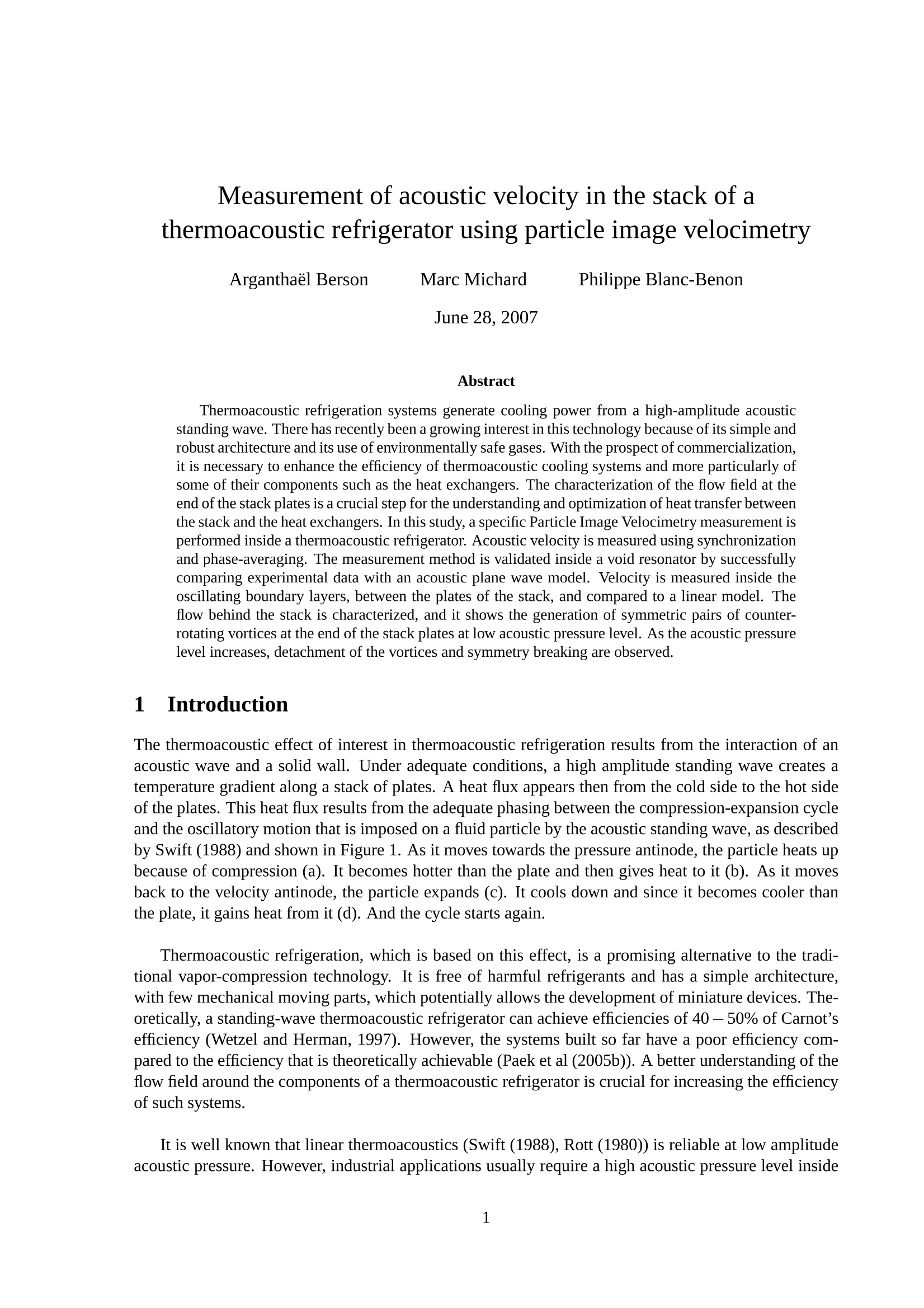
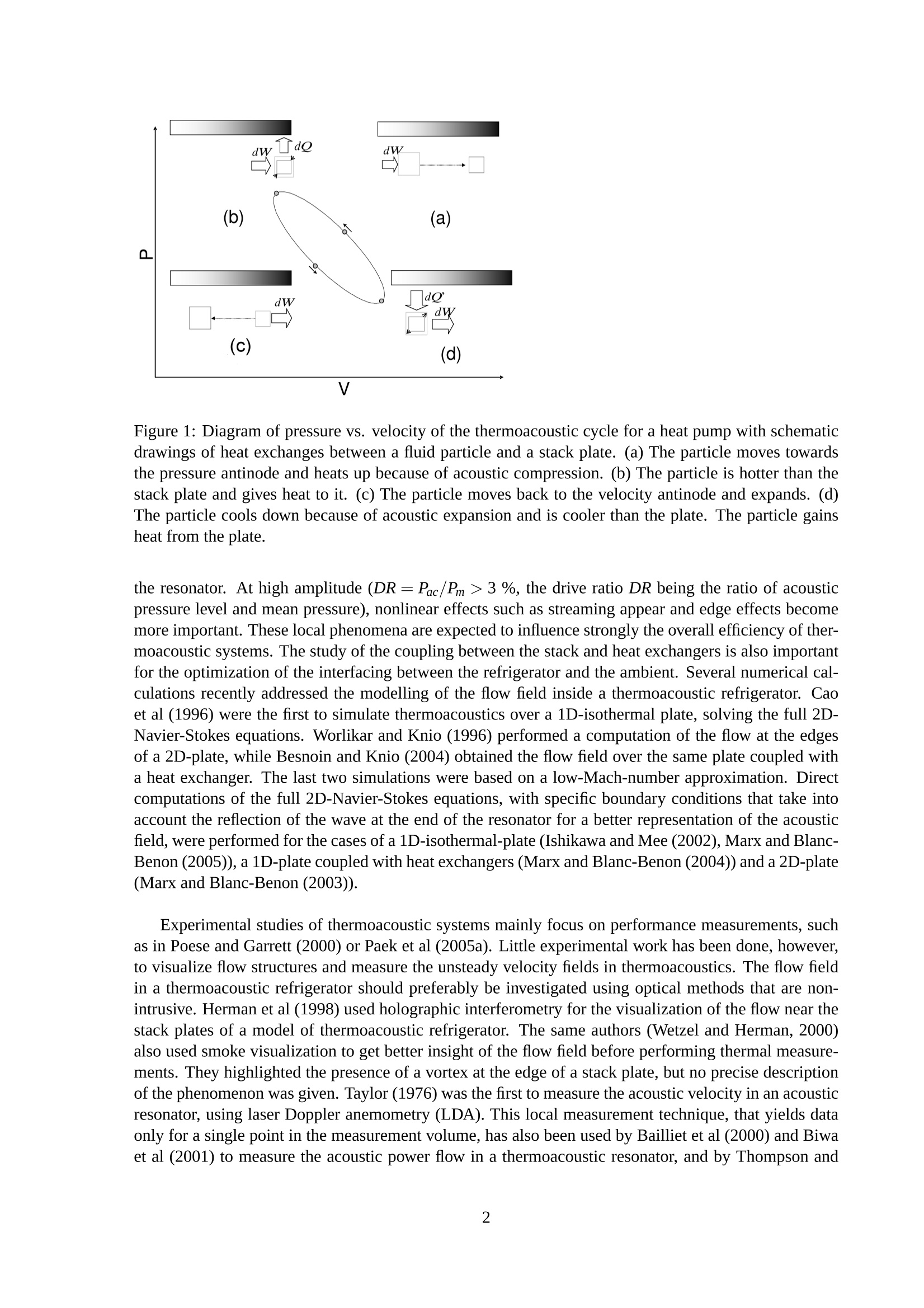
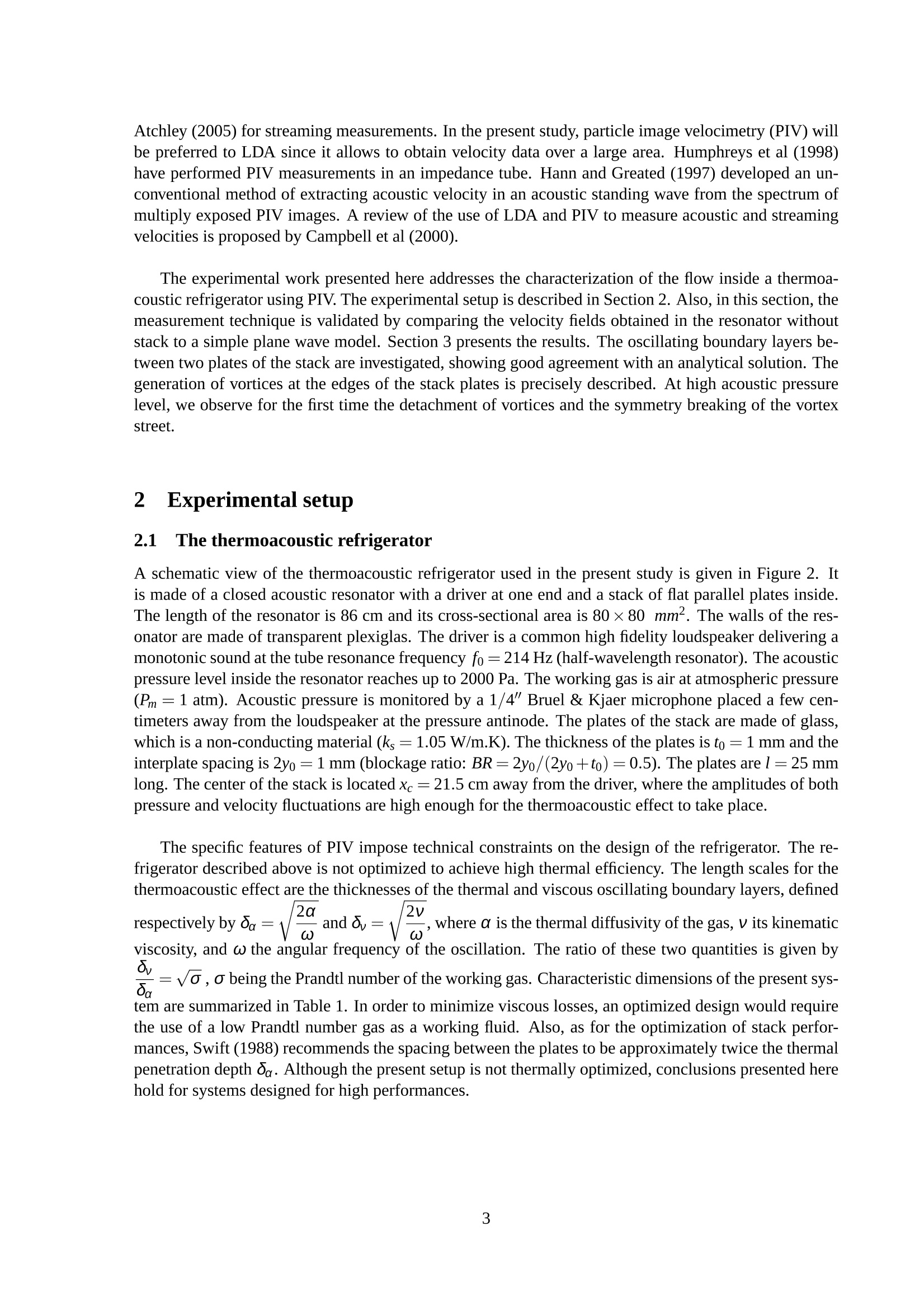
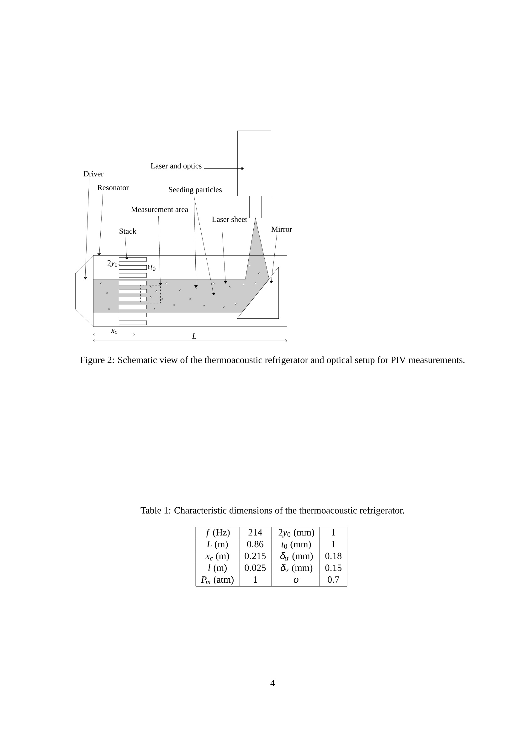
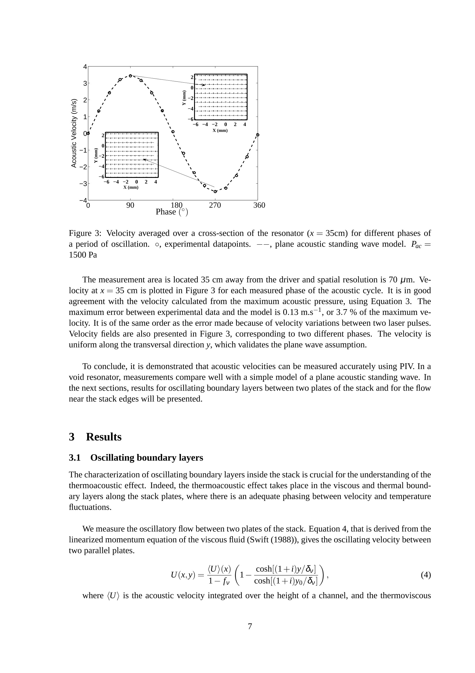
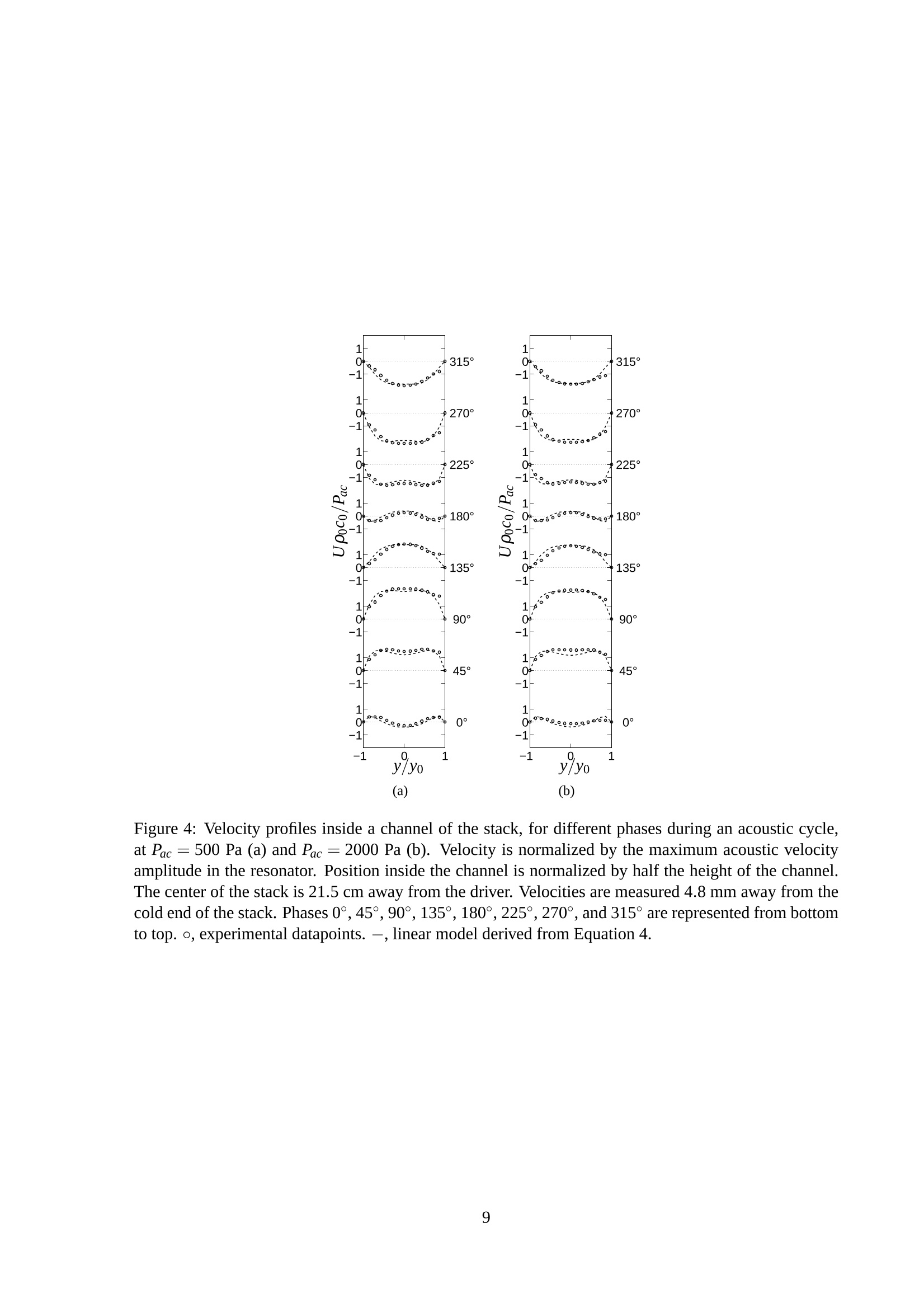
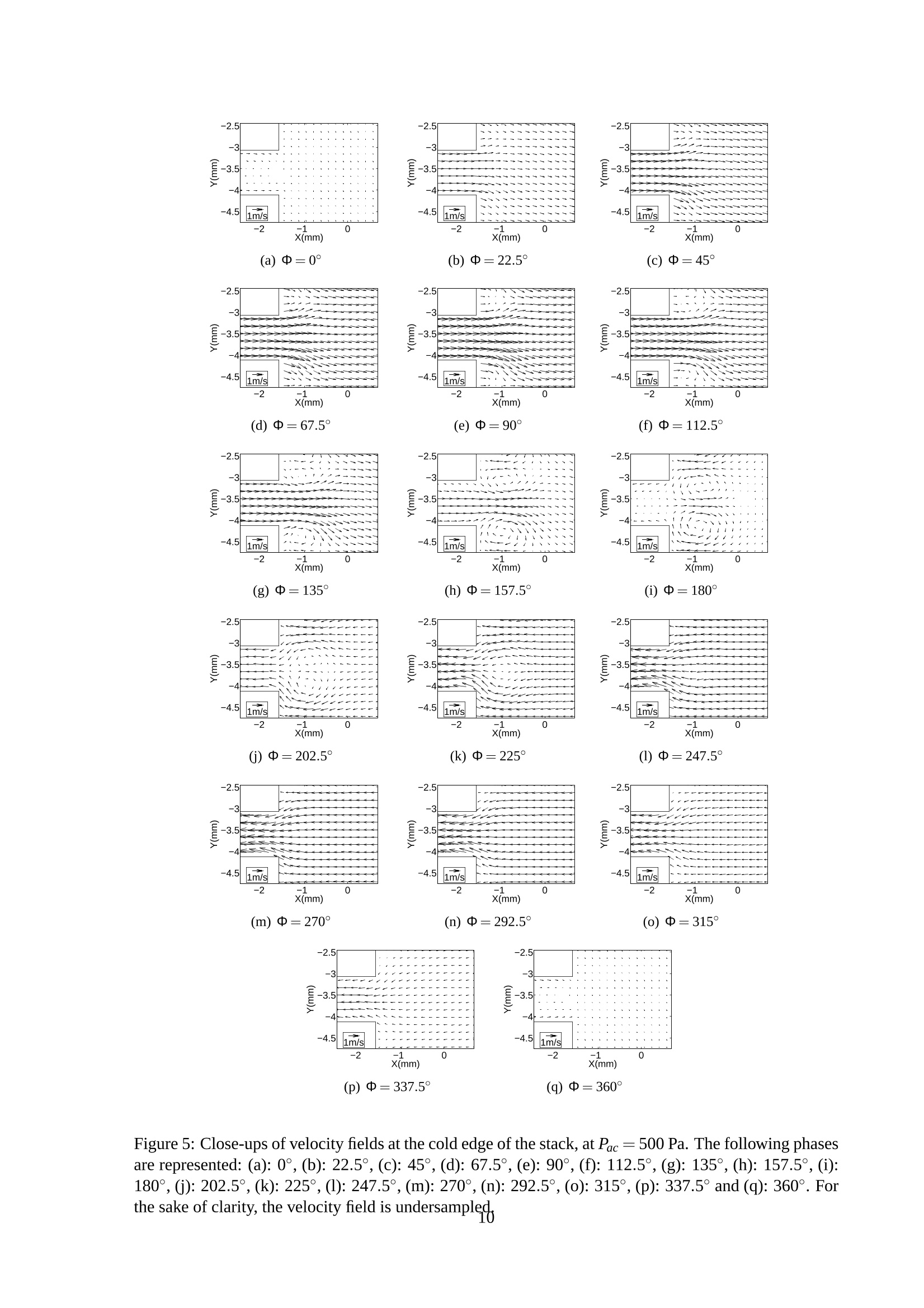
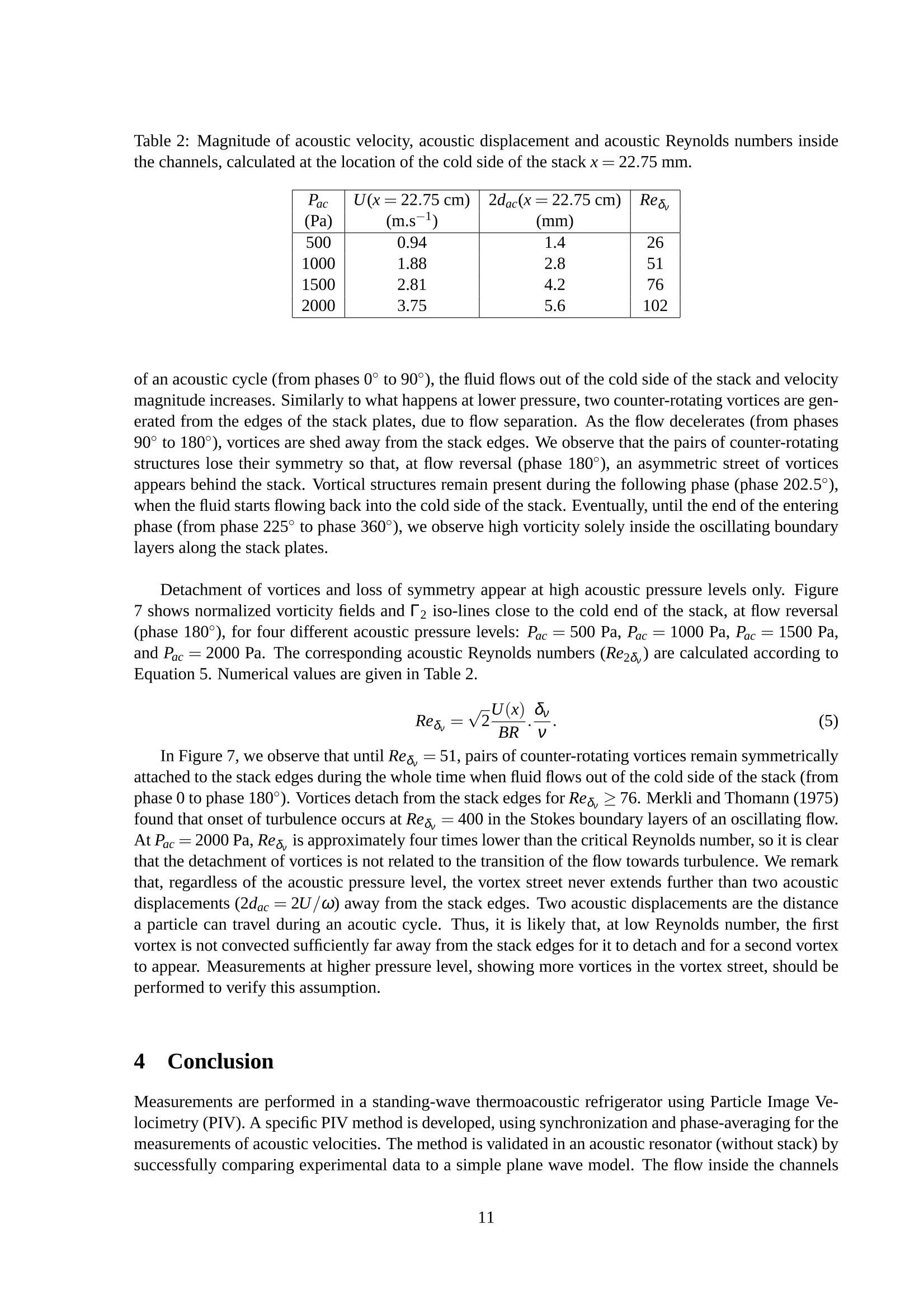
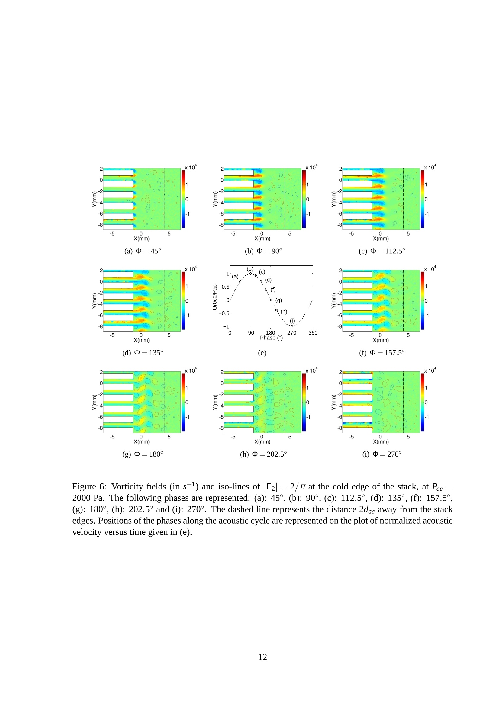
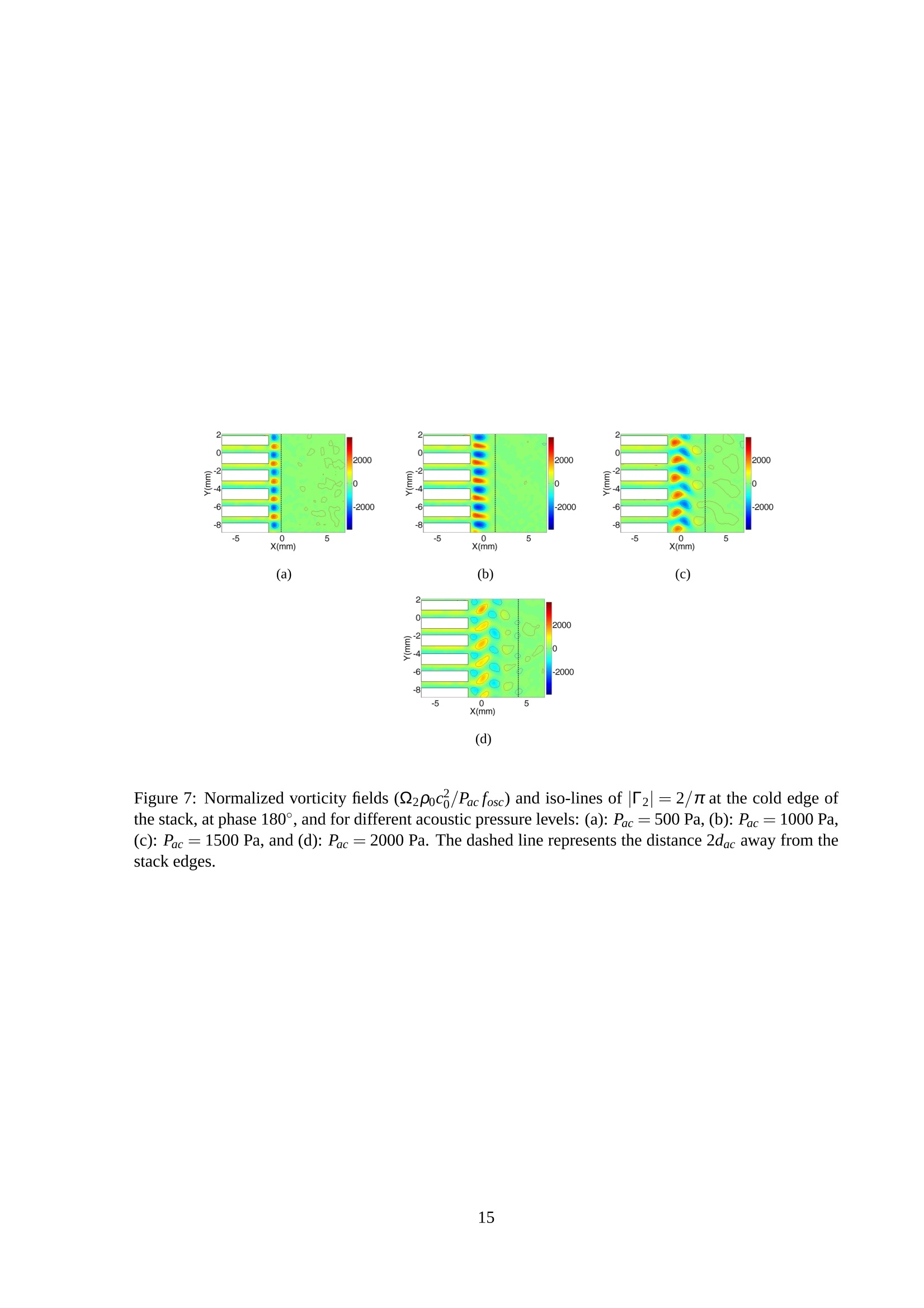
Measurement of acoustic velocity in the stack of athermoacoustic refrigerator using particle image velocimetry Arganthael Berson Marc Michard Philippe Blanc-BenonJune 28， 2007 Abstract Thermoacoustic refrigeration systems generate cooling power from a high-amplitude acousticstanding wave. There has recently been a growing interest in this technology because of its simple androbust architecture and its use of environmentally safe gases. With the prospect of commercialization，it is necessary to enhance the efficiency of thermoacoustic cooling systems and more particularly ofsome of their components such as the heat exchangers. The characterization of the flow field at theend of the stack plates is a crucial step for the understanding and optimization of heat transfer betweenthe stack and the heat exchangers. In this study， a specific Particle Image Velocimetry measurement isperformed inside a thermoacoustic refrigerator. Acoustic velocity is measured using synchronizationand phase-averaging. The measurement method is validated inside a void resonator by successfullycomparing experimental data with an acoustic plane wave model. Velocity is measured inside theoscillating boundary layers， between the plates of the stack， and compared to a linear model. Theflow behind the stack is characterized， and it shows the generation of symmetric pairs of counter-rotating vortices at the end of the stack plates at low acoustic pressure level. As the acoustic pressurelevel increases， detachment of the vortices and symmetry breaking are observed. 1 Introduction The thermoacoustic effect of interest in thermoacoustic refrigeration results from the interaction of anacoustic wave and a solid wall. Under adequate conditions， a high amplitude standing wave creates atemperature gradient along a stack of plates. A heat flux appears then from the cold side to the hot sideof the plates.This heat flux results from the adequate phasing between the compression-expansion cycleand the oscillatory motion that is imposed on a fluid particle by the acoustic standing wave， as describedby Swift (1988) and shown in Figure 1. As it moves towards the pressure antinode， the particle heats upbecause of compression (a). It becomes hotter than the plate and then gives heat to it (b). As it movesback to the velocity antinode， the particle expands (c). It cools down and since it becomes cooler thanthe plate， it gains heat from it (d). And the cycle starts again. Thermoacoustic refrigeration， which is based on this effect， is a promising alternative to the tradi-tional vapor-compression technology. It is free of harmful refrigerants and has a simple architecture，with few mechanical moving parts， which potentially allows the development of miniature devices. The-oretically， a standing-wave thermoacoustic refrigerator can achieve efficiencies of 40 - 50% of Carnot’sefficiency (Wetzel and Herman， 1997). However， the systems built so far have a poor efficiency com-pared to the efficiency that is theoretically achievable (Paek et al (2005b)). A better understanding of theflow field around the components of a thermoacoustic refrigerator is crucial for increasing the efficiencyof such systems. It is well known that linear thermoacoustics (Swift (1988)， Rott (1980)) is reliable at low amplitudeacoustic pressure. However， industrial applications usually require a high acoustic pressure level inside Figure 1： Diagram of pressure vs. velocity of the thermoacoustic cycle for a heat pump with schematicdrawings of heat exchanges between a fluid particle and a stack plate. (a) The particle moves towardsthe pressure antinode and heats up because of acoustic compression. (b) The particle is hotter than thestack plate and gives heat to it.(c) The particle moves back to the velocity antinode and expands. (d)The particle cools down because of acoustic expansion and is cooler than the plate. The particle gainsheat from the plate. the resonator. At high amplitude (DR=Pae/Pm>3 %， the drive ratio DR being the ratio of acousticpressure level and mean pressure)， nonlinear effects such as streaming appear and edge effects becomemore important. These local phenomena are expected to influence strongly the overall efficiency of ther-moacoustic systems. The study of the coupling between the stack and heat exchangers is also importantfor the optimization of the interfacing between the refrigerator and the ambient. Several numerical cal-culations recently addressed the modelling of the flow field inside a thermoacoustic refrigerator. Caoet al (1996) were the first to simulate thermoacoustics over a 1D-isothermal plate， solving the full 2D-Navier-Stokes equations. Worlikar and Knio (1996) performed a computation of the flow at the edgesof a 2D-plate， while Besnoin and Knio (2004) obtained the flow field over the same plate coupled witha heat exchanger. The last two simulations were based on a low-Mach-number approximation. Directcomputations of the full 2D-Navier-Stokes equations， with specific boundary conditions that take intoaccount the reflection of the wave at the end of the resonator for a better representation of the acousticfield， were performed for the cases of a 1D-isothermal-plate (Ishikawa and Mee (2002)， Marx and Blanc-Benon (2005))， a 1D-plate coupled with heat exchangers (Marx and Blanc-Benon (2004)) and a 2D-plate(Marx and Blanc-Benon (2003)). Experimental studies of thermoacoustic systems mainly focus on performance measurements， suchas in Poese and Garrett (2000) or Paek et al (2005a). Little experimental work has been done， however，to visualize flow structures and measure the unsteady velocity fields in thermoacoustics. The flow fieldin a thermoacoustic refrigerator should preferably be investigated using optical methods that are non-intrusive. Herman et al (1998) used holographic interferometry for the visualization of the flow near thestack plates of a model of thermoacoustic refrigerator. The same authors (Wetzel and Herman， 2000)also used smoke visualization to get better insight of the flow field before performing thermal measure-ments. They highlighted the presence of a vortex at the edge of a stack plate， but no precise descriptionof the phenomenon was given. Taylor (1976) was the first to measure the acoustic velocity in an acousticresonator， using laser Doppler anemometry (LDA). This local measurement technique， that yields dataonly for a single point in the measurement volume， has also been used by Bailliet et al (2000) and Biwaet al (2001) to measure the acoustic power flow in a thermoacoustic resonator， and by Thompson and Atchley (2005) for streaming measurements. In the present study， particle image velocimetry (PIV) willbe preferred to LDA since it allows to obtain velocity data over a large area. Humphreys et al (1998)have performed PIV measurements in an impedance tube. Hann and Greated (1997) developed an un-conventional method of extracting acoustic velocity in an acoustic standing wave from the spectrum ofmultiply exposed PIV images. A review of the use ofLDA and PIV to measure acoustic and streamingvelocities is proposed by Campbell et al (2000). The experimental work presented here addresses the characterization of the flow inside a thermoa-coustic refrigerator using PIV. The experimental setup is described in Section 2. Also， in this section， themeasurement technique is validated by comparing the velocity fields obtained in the resonator withoutstack to a simple plane wave model. Section 3 presents the results. The oscillating boundary layers be-tween two plates of the stack are investigated， showing good agreement with an analytical solution. Thegeneration of vortices at the edges of the stack plates is precisely described. At high acoustic pressurelevel， we observe for the first time the detachment of vortices and the symmetry breaking of the vortexstreet. 2 Experimental setup 2.1 The thermoacoustic refrigerator A schematic view of the thermoacoustic refrigerator used in the present study is given in Figure 2. Itis made of a closed acoustic resonator with a driver at one end and a stack of flat parallel plates inside.The length of the resonator is 86 cm and its cross-sectional area is 80×80 mm2. The walls of the res-onator are made of transparent plexiglas. The driver is a common high fidelity loudspeaker delivering amonotonic sound at the tube resonance frequency fo =214 Hz (half-wavelength resonator). The acousticpressure level inside the resonator reaches up to 2000 Pa. The working gas is air at atmospheric pressure(Pm =1 atm). Acoustic pressure is monitored by a 1/4" Bruel & Kjaer microphone placed a few cen-timeters away from the loudspeaker at the pressure antinode. The plates of the stack are made of glass，which is a non-conducting material (ks=1.05 W/m.K). The thickness of the plates is to=1 mm and theinterplate spacing is 2yo=1 mm (blockage ratio： BR=2yo/(2yo+to)=0.5). The plates are l=25 mmlong. The center of the stack is located xc =21.5 cm away from the driver， where the amplitudes of bothpressure and velocity fluctuations are high enough for the thermoacoustic effect to take place. The specific features of PIV impose technical constraints on the design of the refrigerator. The re- frigerator described above is not optimized to achieve high thermal efficiency. The length scales for the thermoacoustic effect are the thicknesses of the thermal and viscous oscillating boundary layers， defined2a 2vrespectively by 8a=and 8v=，w一，h ewhreere aa iis the thermal diffusivity of the gas， v its kinematicviscosity， and ω the angular frequency of the oscillation. The ratio of these two quantities is given by=√o， o being the Prandtl number of the working gas. Characteristic dimensions of the present sys-8tem are summarized in Table 1. In order to minimize viscous losses， an optimized design would requirethe use of a low Prandtl number gas as a working fluid. Also， as for the optimization of stack perfor-mances， Swift (1988) recommends the spacing between the plates to be approximately twice the thermalpenetration depth 8a. Although the present setup is not thermally optimized， conclusions presented herehold for systems designed for high performances. Figure 2： Schematic view of the thermoacoustic refrigerator and optical setup for PIV measurements. Table 1： Characteristic dimensions of the thermoacoustic refrigerator. f (Hz)L (m)xc(m)l (m)Pm (atm) 2140.860.2150.0251 2yo(mm)to (mm)8c (mm)8 (mm) 11 0.180.150.7 2.2 The PIV measuring system Optical setup The optical setup is represented in Figure 2. The camera is a C LaVision FlowMaster 3with a 1280×1024 pix² (8.6×6.9 mm²) CCD sensor. Measurement fields of minimum area 11×9 mm2are obtained with aC Nikon 60 mm lens and extension tubes. The working distance is approximately10 cm from the measurement field and magnification is estimated to be 0.77. The camera is placedperpendicular to the direction of oscillations. The laser sheet is generated by a dual-resonator Nd：YAGlaser with a wavelength of 532 nm， and combined with a cylindrical lens. The time between 2 pulsesis 52 us for 500 Pa， 26 us for 1000 and 1500 Pa， and 13 us for 2000 Pa. It has to be small enoughcompared to the acoustic period (T=4.6 ms) for velocity variations to be negligible between two laserpulses. Close to flow reversal， when time derivative of acoustic velocity is at its maximum， the error dueto velocity variations between two laser pulses is estimated to be 6.6 cm.ss-1 for 500， 1000 and 2000 Pa，and 9.8 cm.s- for 1500 Pa， for measurements made at xc=22.75 cm. These values correspond to 7%of the velocity amplitude at 500 Pa， 3.5% at 1000 and 1500 Pa， and 1.75 % at 2000 Pa. A small and thinmirror， of dimensions 75×75 mm²， thickness 5 mm and with a 45°-angle with respect to the directionof oscillations， is placed inside the resonator to reflect the laser sheet and create the measurement planeperpendicular to the plates of the stack and to the optical axis of the camera. The laser does not illuminatethe edges of the stack directly so that there are no unwanted reflections on the stack plates. The mirroris located far from the stack， inside the opposite half of the resonator， and since its dimensions are smallwith respect to the acoustic wavelength， it does not disturb the acoustic wave. Particle seeding The measurement plane is seeded with paraffin oil smoke generated by a commercialsmoke machine. The smoke is filtered to eliminate large particles. The diameter of the particles rangesfrom 1 to 4 um. According to the characteristics of the optical system and for an aperture of 4 mm，the diameter of a particle image on the sensor is approximately 5 pix which satisfies the requirementsof the PIV software. The smoke is fed inside the resonator through a capillary tube flush-mounted in awall， near the measurement area. Another flush-mounted capillary tube is placed further on the wall. Itsother end is immersed in water in order to maintain constant pressure inside the resonator during smokeinjection. Smoke is injected before turning the loudspeaker on. Acoustic oscillations make the seedinghomogeneous and measurements can be performed. Since we are interested in the characteristics of an unsteady flow， it is necessary to verify that particlesfollow the flow for the frequency range of interest. This will ensure that the measured velocity is in goodagreement with the actual flow field. As proposed in the review by Melling (1997)， we solve the equationof motion of a seeding particle. Considering that the particle density is greater than the fluid densitypp/pf> 1， this equation reduces in our case to where pp， u and dp are the density， dynamic viscosity and diameter of the seeding particle， respec-tively. Uf and Up are instantaneous velocities of the fluid and seeding particle， respectively. The ration=Up/Us of these two velocities is obtained from the solution of Equation 1. Assuming that particlesfollow the flow for n>0.99， the maximum acceptable diameter for a particle of paraffin oil smoke is6.38 um at the frequency of interest (fo =214 Hz). It is greater than the size of the particles introducedinto the resonator. Hence， we conclude that the use of paraffin oil smoke is appropriate for PIV measure-ments in the setup presented here. Data acquisition and processingThe maximum repetition rate of the camera for PIV measurementsis fcam =2 Hz， which is below the frequency of oscillation (fo =214 Hz). This limitation is overcome using phase averaging. Acoustic velocity being periodical， PIV image acquisition is phase-locked withthe voltage feeding the loudspeaker using a TTL triggering signal delivered by the signal generator. Atime lag t between TTL signal and the time when both camera and laser are triggered is defined in thesoftware. By adjusting t， an acoustic cycle is subdivided in 16 equally spaced phases. We define theinitial phase (0°) as the time when velocity is zero and when the fluid flows out of the cold side of thestack during the following half period. Fifty instantaneous velocity fields are measured for each phase，and averaged in order to obtain a phase-averaged velocity field. Velocity fields are processed from the images with the commercial system CLavision Davis 7.0.Multiple iterations with window shift and decreasing window size ensure a high spatial resolution withlow signal-to-noise ratio. As shown by Berson et al (2006)， spatial resolution is a limiting parameterfor a good estimation of space derivatives that are used in the calculation of quantities such as vorticityor viscous dissipation. The size of the final interrogation windows is 16×16 pix² with 50 % overlap，leading to a spatial resolution of 70 um for a measurement area of11×9 mm. OuThe z-composnoennetnt of the vorticity vector z=ar is calculated. The I2 function is alsocomputed to detect vortex boundaries. Let M be a point of the plane， I2 is defined by： where S is a disc of center M. 0 is the angle between x-xandu(M)-u(M)， M’being a point insideS with coordinates x， andi(M) is the velocity at coordinate M. The radius of S is four times the spatialresolution. Subscripts i and j refer to the vector components in the plane. I2 has values between 2/nand 1 when the flow is locally dominated by rotation. T2 function is a nondimensional quantity based onthe topological properties of the flow rather than on its intensity. Thus， it is a powerful tool to detect vor-tex boundaries in a strongly inhomogneous flow such as the present one. More details about I2 functioncan be found in Graftieaux et al (2001). 2.3 Acoustic velocity in the resonator without stack： validation of the measurements The experimental setup presented here has already been validated by Duffourd (2001).In this section， weoperate in the resonator of the thermoacoustic refrigerator without stack. Thus， we consider the resonatoras a closed tube with a piston-like source at the x=0 end. The driver delivers a sinusoidal excitation atthe tube resonance frequency fo=214 Hz. In this configuration， an acoustic standing wave is formedin the resonator. At this range of frequencies， no transversal modes are excited and the acoustic wave isplane. This means that velocity remains constant in a cross-section of the tube (except within the viscousboundary layer close to the walls). The velocity in a cross-section of abscissa x can be deduced from themaximum acoustic pressure inside the resonator as where Pac is the maximum acoustic pressure in the resonator， po is the density of air， co is the celerityof sound in air， k=ω co is the acoustic wavenumber and t is time. The maximum acoustic pressureinside the tube is 1500 Pa. At this level of acoustic pressure， harmonics appear but remain quite low(second harmonic is no more than a few percents of the fundamental). This introduces only a slight errorwhen data are compared to the model without harmonics. Duffourd (2001) extended the model to takeinto account higher harmonics， and found a good agreement with experimental data. Figure 3： Velocity averaged over a cross-section of the resonator (x=35cm) for different phases ofa period of oscillation. o， experimental datapoints.，-一，-， plane acoustic standing wave model. Pac=1500 Pa The measurement area is located 35 cm away from the driver and spatial resolution is 70 um. Ve-locity at x=35 cm is plotted in Figure 3 for each measured phase of the acoustic cycle. It is in goodagreement with the velocity calculated from the maximum acoustic pressure， using Equation 3. Themaximum error between experimental data and the model is 0.13 m.s-l， or 3.7 % of the maximum ve-locity. It is of the same order as the error made because of velocity variations between two laser pulses.Velocity fields are also presented in Figure 3， corresponding to two different phases. The velocity isuniform along the transversal direction y， which validates the plane wave assumption. To conclude， it is demonstrated that acoustic velocities can be measured accurately using PIV. In avoid resonator， measurements compare well with a simple model of a plane acoustic standing wave. Inthe next sections， results for oscillating boundary layers between two plates of the stack and for the flownear the stack edges will be presented. 3 Results 3.1 Oscillating boundary layers The characterization of oscillating boundary layers inside the stack is crucial for the understanding of thethermoacoustic effect. Indeed， the thermoacoustic effect takes place in the viscous and thermal bound-ary layers along the stack plates， where there is an adequate phasing between velocity and temperaturefluctuations. We measure the oscillatory flow between two plates of the stack. Equation 4， that is derived from thelinearized momentum equation of the viscous fluid (Swift (1988))， gives the oscillating velocity betweentwo parallel plates. where (U) is the acoustic velocity integrated over the height of a channel， and the thermoviscous function ft is defined asftanh(1+i)yo/8 The phase-averaged velocity profiles measured in a stack channel are given in Figure 4， for eightphases of the acoustic period， and two acoustic pressure levels： 500 Pa and 2000 Pa. Measurements areperformed inside the cross-section of a channel located 4.8 mm away from the cold edges of the plates.The centre of the stack is placed at xc =21.5 cm. Both end points of each velocity profile belong to theplates. They have zero velocity and are plotted for reference. Spatial resolution is 80 um. A precisedescription of the flow close to the wall would require a better spatial resolution， but this is beyond thescope of this paper. The flow inside the channel is laminar and it is strongly influenced by viscous effects. Indeed，theviscous boundary layers occupy no less than approximately one third of the space between two plates.When the sign of the acoustic velocity changes (at D=0°and①=180°)， flow reversal appears first inthe viscous boundary layer， where the flow has less inertia. Hence， the fluid in the middle of the channeland the fluid close to the plates flow in opposite ways. These measurements are in accordance with themodel described by Equation 4. Comparisons between velocity profiles measured with PIV and theoretical velocity profiles calcu-lated from Equation 4 show good qualitative agreement. At low acoustic pressure level (500 Pa)， dis-crepancies between the measurements and the linear model are within experimental error. However， thelinear model is less accurate at higher level (2000 Pa). This is likely to be due to nonlinearities that startto appear as acoustic load increases. At even higher acoustic pressure level， one should expect effectssuch as streaming or turbulent structures to appear inside these boundary layers. This will affect theefficiency of the system. 3.2 Velocity fields at the edges of stack plates Blanc-Benon and Marx (2005) have shown that the topology of the flow behind the stack has a stronginfluence on the heat flux close to the edges of the stack plates. The aerodynamic field behind the stackdepends on its geometry. Experiments have been performed previously with this experimental setup fordifferent stack geometries， at low acoustic pressure level (Pac ≤ 1500 Pa)， and compared to numericalsimulations (Blanc-Benon et al(2003)， Marx (2003)). In this paper we focus on the stack described inSection 2.1， whose blockage is high and whose plates are thick. The center of the stack is located atxc=21.5 cm， and spatial resolution of the measurements is 85 um. Close-ups of velocity fields at the edge of the stack plates， at Pac = 500 Pa are given in Figure 5 forselected time instants during an acoustic cycle. In this section， we focus on the cold side of the stack，but the same analysis remains valid for the hot side. During the phases when the fluid flows out of thestack (from phases 0° to 180°)， the fluid rolls up around the sharp edges of the stack plates， due to flowseparation. This mechanism leads to the generation of two counter-rotating vortices behind each stackplate. These vortices are symmetric and remain attached to the edges of the stack plates. At phases202.5° and 225°， the fluid is sucked back between the plates. The persistance of the formerly generatedvortices makes the flow slightly rotationnal， and creates areas of low velocity just behind the channel.From phases 247.5° to 360°， the fluid enters the channel， flowing around the plate edges. Fluid velocityis higher whithin the channel than outside because of the blockage created by the presence of the stackin the resonator. At higher acoustic pressure level， the topology of the flow is different. Figure 6 shows vorticity fieldsand I2 iso-lines behind stack plates for 7 different phases of an acoustic period. Figure 6(e) helps to sit-uate the phases on an acoustic period. Acoustic pressure level is Pac =2000 Pa. During the first quarter Figure 4： Velocity profiles inside a channel of the stack， for different phases during an acoustic cycle，at Pac=500 Pa (a) and Pac=2000 Pa (b). Velocity is normalized by the maximum acoustic velocityamplitude in the resonator. Position inside the channel is normalized by half the height of the channel.The center of the stack is 21.5 cm away from the driver. Velocities are measured 4.8 mm away from thecold end of the stack. Phases0°，45°，90°，135°，180°，225°，270°， and 315° are represented from bottomto top. o， experimental datapoints. -，linear model derived from Equation 4. are represented： (a)： 0，(b)：22.5°， (c)： 45°， (d)： 67.5°， (e)： 90°， (f)： 112.5°，(g)：135°，(h)： 157.5°，(1)：180°， ()： 202.5， (k)： 225°，(1)： 247.5°， (m)： 270°， (n)： 292.5°， (0)： 315°， (D)： 337.5° and (q)： 360°. Forthe sake of clarity， the velocity field is undersampled， Table 2： Magnitude of acoustic velocity， acoustic displacement and acoustic Reynolds numbers insidethe channels， calculated at the location of the cold side of the stackx=22.75 mm. Pac(Pa) U(x=22.75 cm)(m.s) 2dac(x=22.75 cm)(mm) Res 500 0.94 1.42.8 2651 1000 1.88 1500 2.81 3.75 4.2 5.6 76 2000 102 of an acoustic cycle (from phases 0° to 90°)， the fluid flows out of the cold side of the stack and velocitymagnitude increases. Similarly to what happens at lower pressure， two counter-rotating vortices are gen-erated from the edges of the stack plates， due to flow separation. As the flow decelerates (from phases90° to 180°)， vortices are shed away from the stack edges. We observe that the pairs of counter-rotatingstructures lose their symmetry so that， at flow reversal (phase 180°)， an asymmetric street of vorticesappears behind the stack. Vortical structures remain present during the following phase (phase 202.5°)，when the fluid starts flowing back into the cold side of the stack. Eventually， until the end of the enteringphase (from phase 225° to phase 360°)， we observe high vorticity solely inside the oscillating boundarylayers along the stack plates. Detachment of vortices and loss of symmetry appear at high acoustic pressure levels only. Figure7 shows normalized vorticity fields and I2 iso-lines close to the cold end of the stack， at flow reversal(phase180°)， for four different acoustic pressure levels： Pac = 500 Pa， Pac = 1000 Pa， Pac = 1500 Pa，and Pac =2000 Pa. The corresponding acoustic Reynolds numbers (Re28) are calculated according toEquation 5. Numerical values are given in Table 2. In Figure 7， we observe that until Res， = 51， pairs of counter-rotating vortices remain symmetrically attached to the stack edges during the whole time when fluid flows out of the cold side of the stack (fromphase 0 to phase 180°). Vortices detach from the stack edges for Res ≥76. Merkli and Thomann (1975)found that onset of turbulence occurs at Res，= 400 in the Stokes boundary layers of an oscillating flow.At Pac=2000 Pa， Res， is approximately four times lower than the critical Reynolds number， so it is clearthat the detachment of vortices is not related to the transition of the flow towards turbulence. We remarkthat， regardless of the acoustic pressure level， the vortex street never extends further than two acousticdisplacements (2dac =2U/ω) away from the stack edges. Two acoustic displacements are the distancea particle can travel during an acoutic cycle. Thus， it is likely that， at low Reynolds number， the firstvortex is not convected sufficiently far away from the stack edges for it to detach and for a second vortexto appear. Measurements at higher pressure level， showing more vortices in the vortex street， should beperformed to verify this assumption. 4 Conclusion Measurements are performed in a standing-wave thermoacoustic refrigerator using Particle Image Ve-locimetry (PIV). A specific PIV method is developed， using synchronization and phase-averaging for themeasurements of acoustic velocities. The method is validated in an acoustic resonator (without stack) bysuccessfully comparing experimental data to a simple plane wave model. The flow inside the channels (g)D=180° (h)D=202.5° Figure 6： Vorticity fields (in s-l) and iso-lines of T2|=2/n at the cold edge of the stack， at Pac =2000 Pa. The following phases are represented： (a)： 45°， (b)：90°， (c)： 112.5°，(d)： 135°，(f)： 157.5°，(g)： 180°，(h)：202.5°and (i)： 270°. The dashed line represents the distance 2dac away from the stackedges.Positions of the phases along the acoustic cycle are represented on the plot of normalized acousticvelocity versus time given in (e). of the stack is studied and shows good quantitative agreement at Pac =500 Pa. The measuring methodis validated and shows the limitations of the linear model at higher acoustic pressure level， when nonlin-earities appear. Acoustic velocity fields behind the stack plates are characterized. Vortices appear duringthe half period of the acoustic cycle when the fluid flows out of the stack. At low acoustic pressure level，counter-rotating vortices are generated at the edges of the plates. They are symmetrical and remain at-tached to the plates. With increasing acoustic pressure level， structures detach and create an asymmetricstreet of vortices. Regardless of the pressure level， vortices are not shed further than two acoustic dis-placements away from the stack edges. In future studies， higher acoustic pressure levels will be requiredfor a more precise description of the mechanisms of vortex shedding behind the stack plates. Part of this work was supported by ANR (project MicroThermoAc NT051_42101). The authors arealso grateful to N. Grosjean， J.-M. Perrin and Ch. Nicot for their technical assistance during all the stagesof this experimental work. References Bailliet H， Lotton P， Bruneau M， Gusev V， Valiere JC， Gazenbel B (2000) Acoustic power flow measure-ment in a thermoacoustic resonator by means of Laser Doppler Anemometry (LDA) and microphonicmeasurement. Applied Acoustics 60(1)：1-11 Berson A， Blanc-Benon P， Michard M (2006) Ecoulements secondaires aux extremites du stack d'unrefrigerateur thermoacoustique ： mesure des champs de vitesse oscillante a l’aide de la PIV. In： 8èmeCongres Francais d'Acoustique (CD-ROM)，Tours， France， pp 749-752 ( Besnoin E， Knio OM (2004) Numerical study of thermoacoustic heat exchangers. Acta Acustica united with Acustica 90：432-444 ) Biwa T， Ueda Y， Yazaki T， Mizutani U (2001) Work flow measurements in a thermoacoustic engine.Cryogenics 41(5)：305-310 Blanc-Benon P， Marx D (2005) Nonlinear effects in standing wave thermoacoustic resonator. In： Firstjoint workshop of Russian Acoustical Society (RAS) and French Acoustical Society (SFA) on“Highintensity acoustic waves in modern technological and medical applications”， special session of theXVI Meeting of the RAS， Moscow， Russia， pp 57-65 Blanc-Benon P， Besnoin E， Knio OM (2003) Experimental and computational visualization of the flowfield in a thermoacoustic stack. CR Mecanique 331：17-24 Campbell M， Cosgrove JA， Greated CA， Jack S， Rockliff D (2000) Review of LDA and PIV applied tothe measurement of sound and acoustic streaming. Opt Laser Technol 32：629-639 Cao N， Olson JR， Swift GW， Chen S (1996) Energy flux density in a thermoacoustic couple. J AcoustSoc Am 99(6)：3456-3464 Duffourd S (2001) Refrigerateur thermoacoustique ： etudes analytiques et experimentales en vue d'uneminiaturisation 2001-06. PhD thesis， Ecole Centrale de Lyon Graftieaux L， Michard M， Grosjean N (2001) Combining PIV， POD and vortex identification algorithmsfor the study of unsteady turbulent swirling flows. Meas Sci Technol 12：1422-1429 Hann DB， Greated CA (1997) Particle image velocimetry fort the measurement of mean and acousticparticle velocities. Meas Sci Techno1 8：656-660 Herman C， Kang E， Wetzel M (1998) Expanding the applications of holographic interferometry to thequantitative visualization of oscillatory thermofluid processes using temperature as tracer. Exp Fluids24：431-446 Humphreys WM， Bartram SM， Parrott TL， Jones MG (1998) Digital PIV measurements of acousticparticle displacements in a normal incidence impedance tube. In： 20th AIAA Advanced Measurementand Ground Testing Technology Conference， Albuquerque， NM Ishikawa H， Mee DJ (2002) Numerical investigations of flow and energy fields near a thermoacousticcouple. J Acoust Soc Am 111(2)：831-839 Marx D (2003) Simulation numerique d'un refrigerateur thermoacoustique 2003-34. PhD thesis， EcoleCentrale de Lyon Marx D， Blanc-Benon P (2003) Numerical simulation of hydrodynamic and thermal effects around a 2-Dstack plate in a thermoacoustic refrigerator. J Acoust Soc Am 114(4)：2329 Marx D， Blanc-Benon P (2004) Numerical simulation of stack-heat exchangers coupling in a thermoa-coustic refrigerator. AIAA Journal 42(7)：1338-1347 Marx D， Blanc-Benon P (2005) Computation of the temperature distortion in the stack of a standing-wavethermoacoustic refrigerator. J Acoust Soc Am 118(5)：2993-2999 Melling A (1997) Tracer particles and seeding for particle image velocimetry. Meas Sci Technol 8：1406-1416 ( Merkli P， Thomann H ( 1975) Transition to turbulence in osc i llating pipe flow. J Fluid Mech 68(3)：567-575 ) ( Paek I， Braun JE， Mongeau L ( 2 005a) Char a cterizing heat transfer coefficients for h eat exchangers instanding wave thermoacoustic coolers. J Acoust Soc Am 1 18(4)：2271-2280 ) ( Paek I， Braun JE， Mongeau L (2005b) Second law performance of thermoacoustic systems. J Acoust SocAm 118(3)：1892 ) ( Poese ME， Garrett SL (2000) Performance measurements on a thermoacoustic refrigerator driven at highamplitudes. J Acoust Soc Am 107(5)：2480-2486 ) ( Rott N (1980) Thermoacoustics. Adv Appl Mech 20：135-175 ) ( Swift GW (1988) Thermoacoustic engines. J Acoust Soc A m 84(4)：1145-1180 ) ( T aylor KJ (1976) Absolute measurement of acoustic particle velocity. J Acoust Soc Am 59 ( 3)：691-694 ) ( Thompson MW， Atchley AA (2005) Simultaneous measurement of acoustic and streaming velocities in a standing wave using laser Doppler anemometry. J Acoust Soc Am 1 17(4)：1828-1838 ) Wetzel M， Herman C (1997) Design optimization of thermoacoustic refrigerators. Int J Refrig 20(1)：3-21 Wetzel M， Herman C (2000) Experimental study of thermoacoustic effects on a single plate part I： Tem-perature fields. Heat and Mass Transfer 36：7-20 ( Worlikar A， K nio O (1996) N u merical simulation o f a t h ermoacoustic r e frigerator. J Comput P hys 127：424-451 ) 一EE> Figure 7： Normalized vorticity fields (Q2poc/Pac.fosc) and iso-lines of |T2|=2/n at the cold edge ofthe stack， at phase 180°， and for different acoustic pressure levels： (a)： Pac =500 Pa，(b)： Pac =1000 Pa，(c)： Pac=1500 Pa， and (d)： Pac =2000 Pa. The dashed line represents the distance 2dac away from thestack edges.