


方案详情
文
This paper presents high speed Particle Image Velocimetry (PIV) experiments on small-scale, steep,
breaking waves forced by shoaling the waves up an angled slope to a level plateau, in a lidded tank with an initially
quiescent air-side. Both spilling and plunging breakers are considered. A PIV system, using a high speed digital
video camera at up to 500 frames per second, was used to obtain quantitative data on both the air and water side of
the free surface interface. Waves are generated by a computer controlled, paddle-type wave maker at one end of
long, narrow acrylic tank. In order to obtain breaking waves on a small scale, surface tension was lowered by
mixing isopropyl alcohol with distilled water. Surface tension characteristics of the water-IPA mixture are also
presented herein. To perform high speed PIV measurements, a low-cost, Lasiris Magnum, near-IR, TTL diode line
generator laser is used to form the light sheet. To seed the water, traditional silver coated hollow-glass spheres
were used. While seeding in the water was quite straight-forward, seeding in the air was quite complex. In order
not to adversely affect the surface tension, a water-based fog was used to seed the air. Qualitative visualizations and
PIV show the formation of the vortex aft of the breaking wave and reveal strong counterclockwise vorticity in the air
side of the interface. Results for the plunging breaking wave case are presented herein and compared with
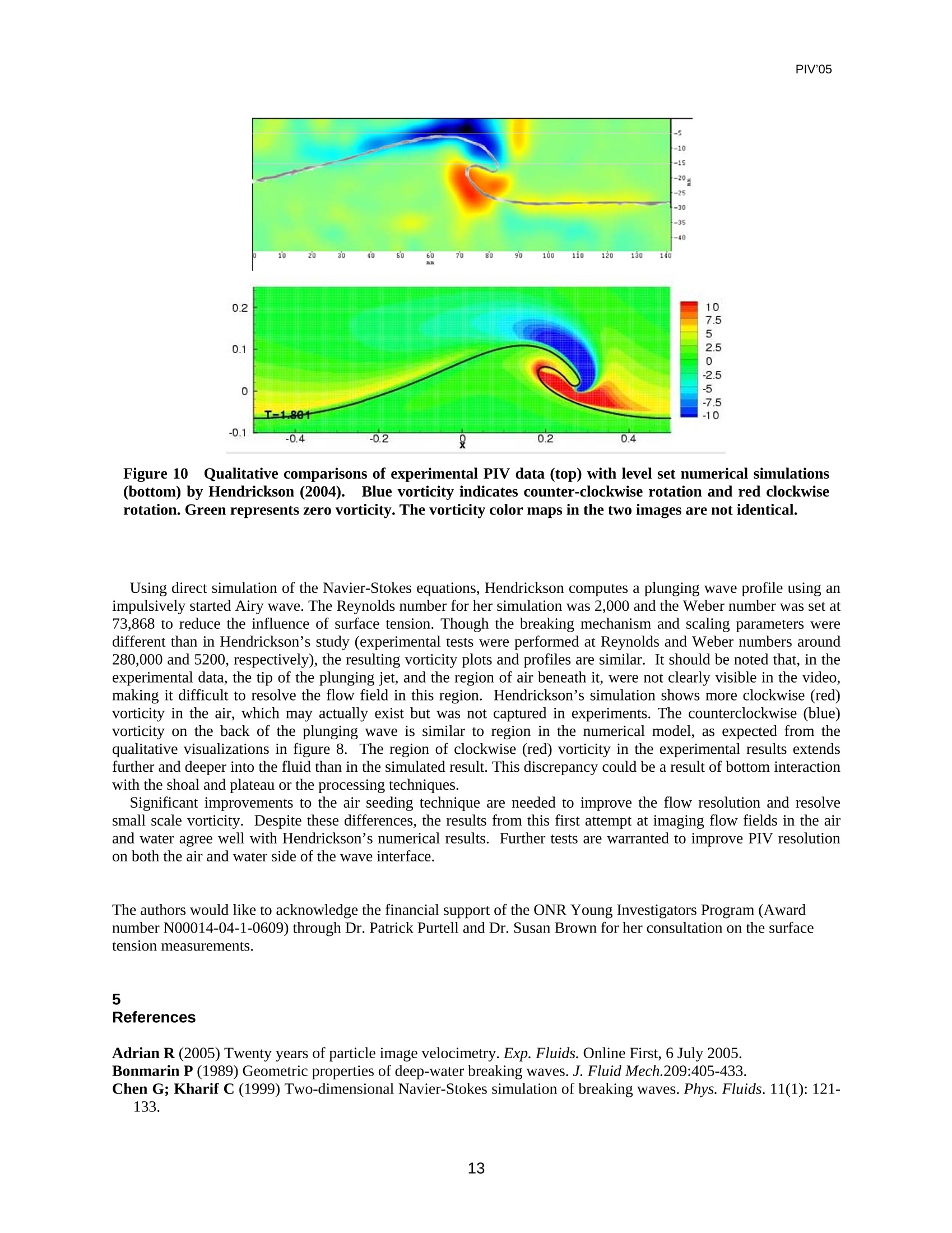
numerical results from Hendrickson (2004).
方案详情

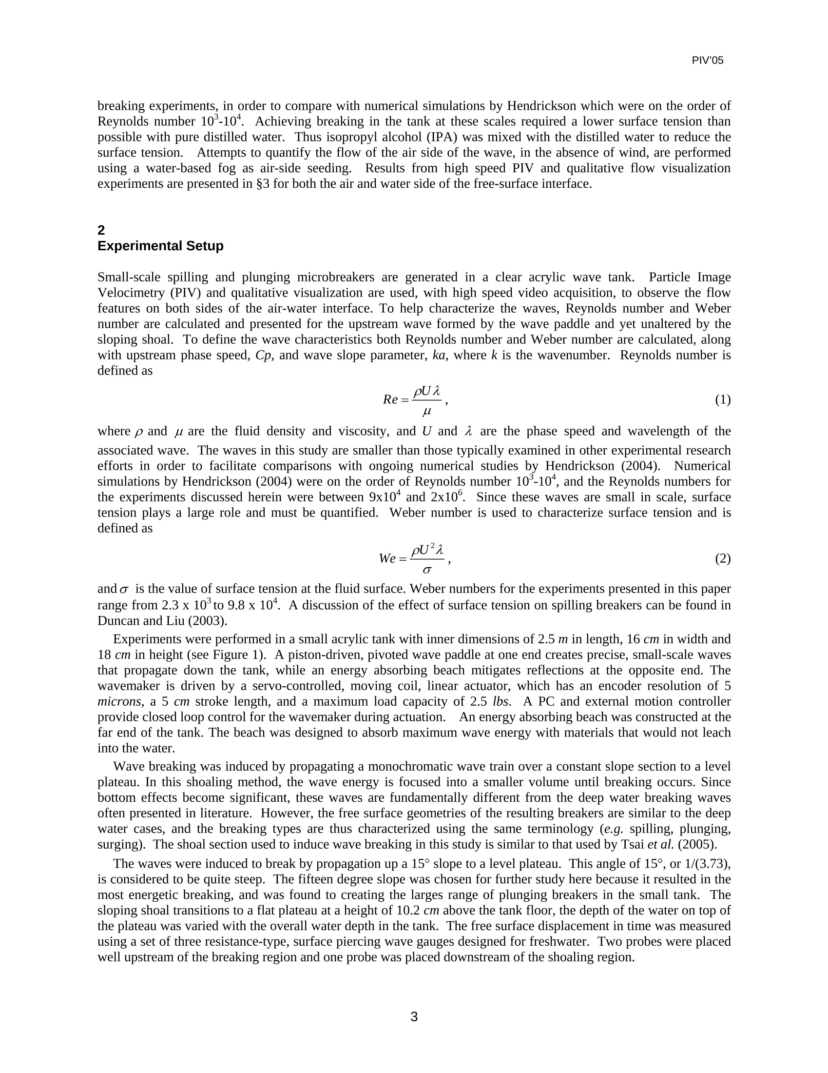
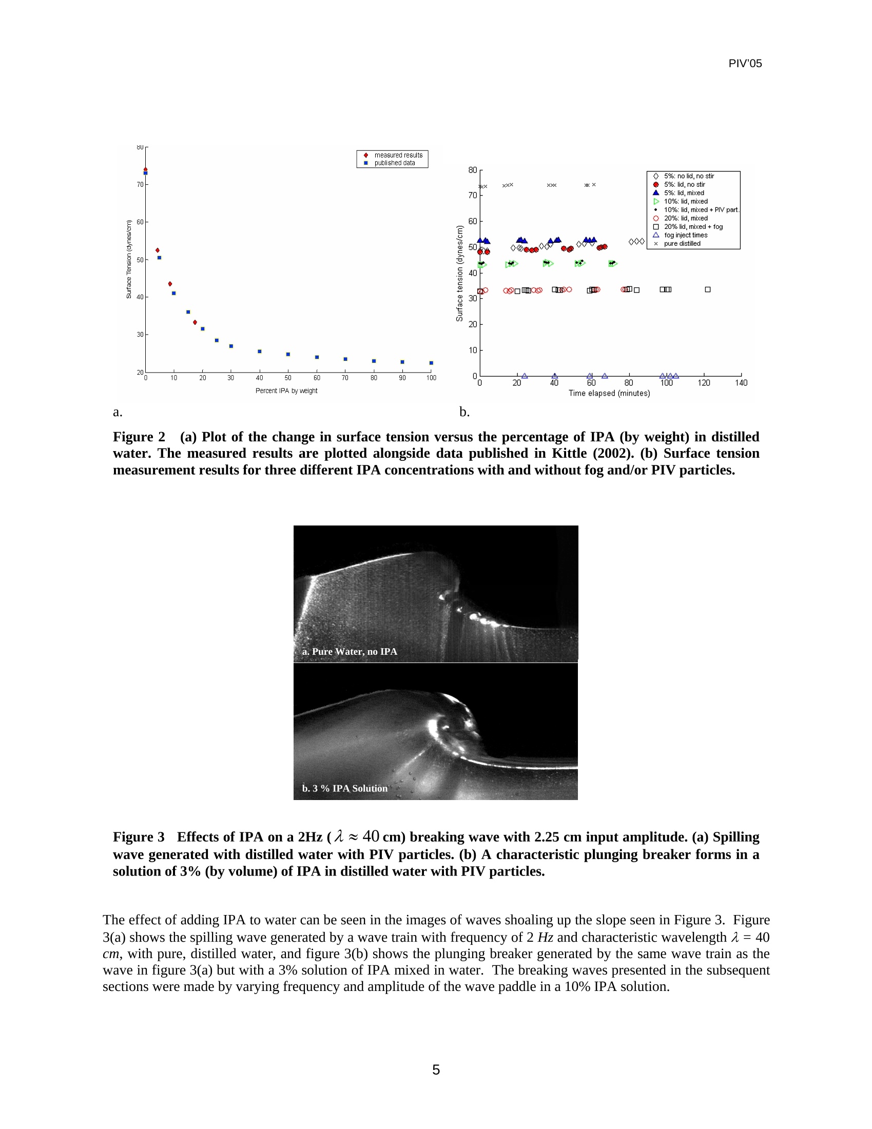
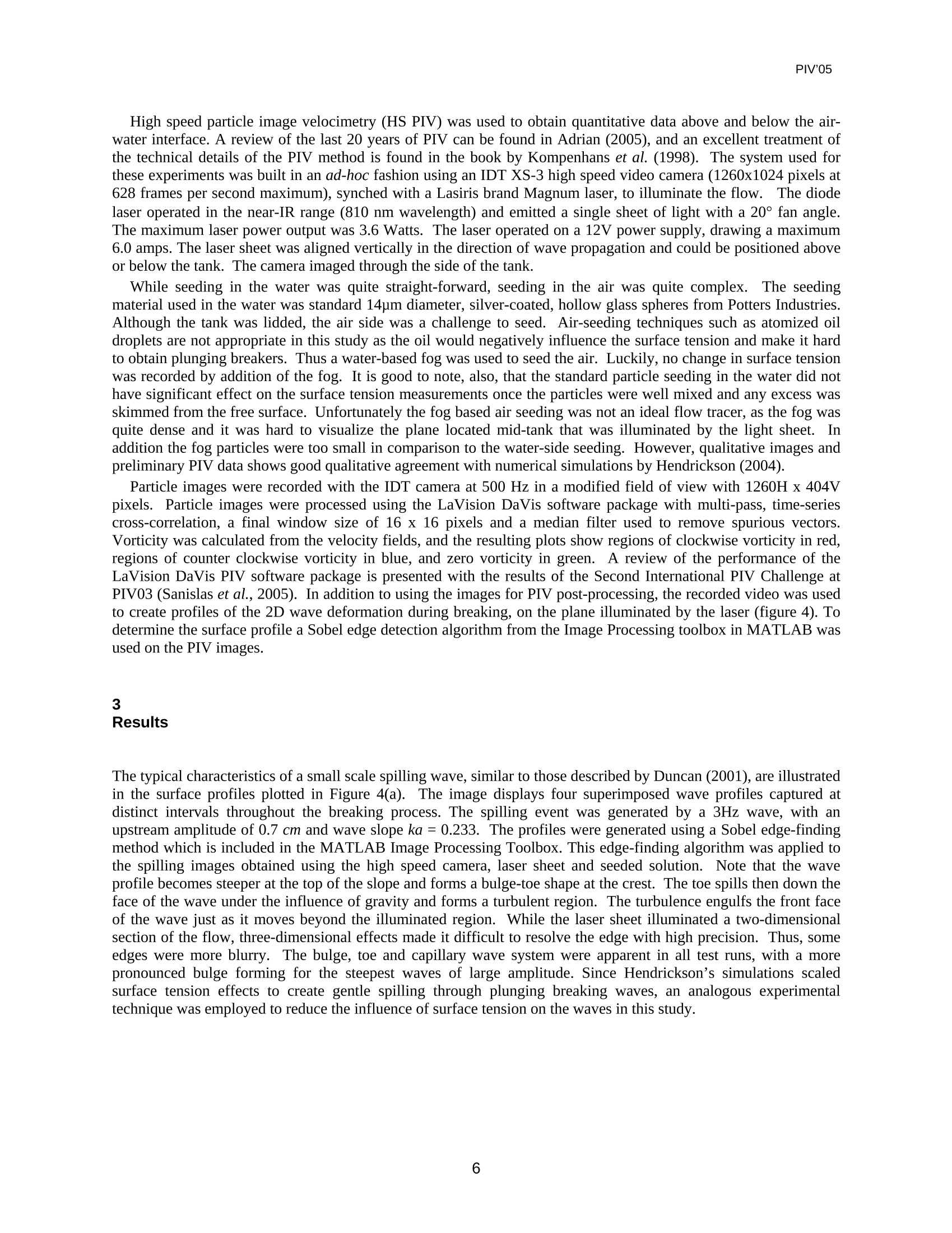
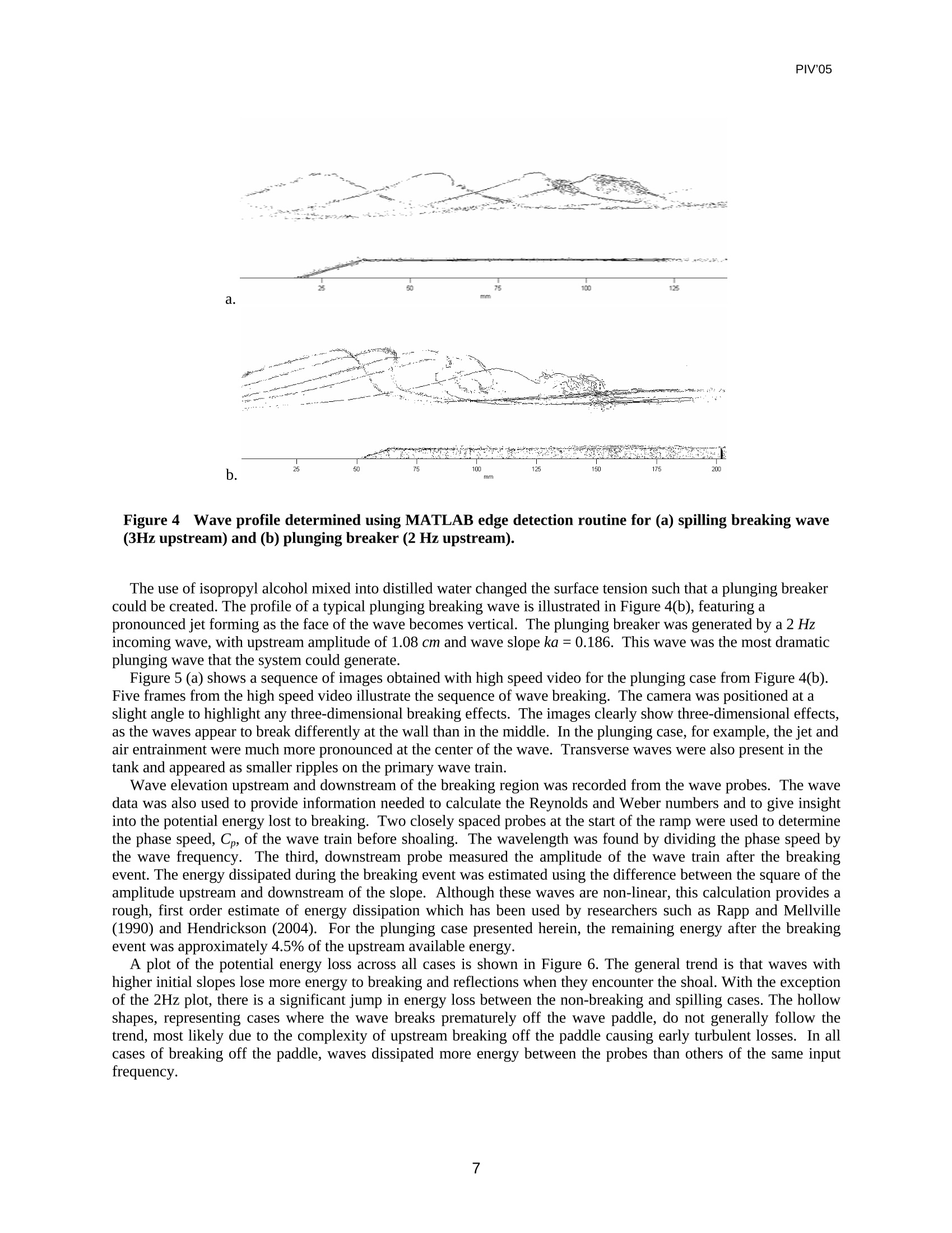
6th International Symposium on Particle Image VelocimetryPIV'05 Paper nnnnPasadena, California, USA, September 21-23, 2005 PIV'05 High Speed PIV of Breaking Waves on Both Sides of the Air-Water Interface A.H. Techet, A.K. McDonald Abstract This paper presents high speed Particle Image Velocimetry (PIV) experiments on small-scale, steep,breaking waves forced by shoaling the waves up an angled slope to a level plateau, in a lidded tank with an initiallyquiescent air-side. Both spilling and plunging breakers are considered. A PIV system, using a high speed digitalvideo camera at up to 500 frames per second, was used to obtain quantitative data on both the air and water side ofthe free surface interface. Waves are generated by a computer controlled, paddle-type wave maker at one end oflong, narrow acrylic tank...In order to obtain breaking waves on a small scale, surface tension was lowered bymixing isopropyl alcohol with distilled water. Surface tension characteristics of the water-IPA mixture are alsopresented herein. To perform high speed PIV measurements, a low-cost, Lasiris Magnum, near-IR, TTL diode linegenerator laser is used to form the light sheet.To seed the water, traditional silver coated hollow-glass sphereswere used. While seeding in the water was quite straight-forward, seeding in the air was quite complex. In ordernot to adversely affect the surface tension, a water-based fog was used to seed the air. Qualitative visualizations andPIV show the formation of the vortex aft of the breaking wave and reveal strong counterclockwise vorticity in the airside of the interface. Results for the plunging breaking wave case are presented herein and compared withnumerical results from Hendrickson (2004). 1 Introduction Wave breaking on the surface of the ocean results in significant transfer of mass, momentum, heat and energy acrossthe air-sea interface. ]Breaking waves contribute significant dynamic loading to offshore platforms and otheroffshore structures, and these loads can cause failure due to fatigue or sheer magnitude of the wave force. On aglobal scale, breaking waves can influence atmospheric and oceanic circulations.Turbulence and bubbleentrainment from broken waves enhance the gas transfer from the air to the water in addition to dissipating surfaceenergy. Each of these changes has a direct influence on the circulations which effect global climate; the extent towhich wave breaking plays a role in this process is not fully resolved.Understanding the physics of thesephenomena remains a challenge, as both the measurement and simulation of the relevant processes are highlycomplex. In order to more clearly understand the whole picture, and to generate accurate models of the air-sea exchangeprocesses during wave breaking events, experiments and simulations that consider the physics on both the air andwater-side of the air-sea interface are warranted. Recent numerical studies have begun to investigate the air-watercoupling during the breaking process, in the absence of ambient wind (e.g. Chen et al. 1999, Hendrickson 2004), butrelatively few experimental studies have looked at flow on both sides of this interface in the absence of wind. The dynamics of breaking waves have been the subject of many researchers through the decades. Melville (1996)offers an extensive review of the different breaking wave geometries, wave breaking mechanisms, and evolution ofthe wave profile for deep water waves, and Peregrine (1983) offers a similar review for near-shore breaking waves.Duncan (2001) presents a recent review of existing work in breaking waves, focusing predominately on spillingbreakers and highlighting the effect of surface tension on the breaking process.A recent collection of papersdiscussing research using PIV to study water waves can be found in Grue et al. (2004). PIV has been widely used toinvestigate velocities and turbulence under water waves (e.g. Perlin et al. 1996, Dabiri and Gharib 1997, Dong et al.1997, Peirson 1997, Melville et al. 2002). ( A .H. Techet, A.K. McDonald, C e nter for Ocean Engineering, Department of Mechanical Engineering, Massachusetts Ins t itute of Technology,Cambridge, MA 02139, USA ) Breaking waves can be classified as plunging, spilling, surging, or collapsing breakers, though deep water wavesinclude only the spilling and plunging types of breaking. Plunging waves feature the formation of a jet at the crestthat projects out from the front face and impacts the free surface with a splash at or below the mean water level. Asthe front face of the wave overturns, air is entrained and a two-phase turbulent flow ensues beneath the surface. Inthe more gentle case, spilling breaking waves begin with a small rough zone or bulge forming on the forward tip ofthe crest. Depending upon the scale, this bulge can include bubbles and droplets or, for smaller scales, a smoothbulge with a train of capillary waves developing beneath it. The turbulent bulge grows by spreading down the frontslope and engulfing the face of the wave. Surging and collapsing waves occur at the shoreline and are closelyrelated. Reflections are significant in these shallow water events. In surging breaking, there is no significantdisturbance in the wave profile except at the moving shoreline. The collapsing wave combines characteristics ofboth surging and plunging breakers, whereby a plunging jet forms on the lower portion of the face of an otherwisesurging wave. Neither collapsing nor surging waves were examined in this study. In addition to their geometry and kinematics, breaking waves are classified by their temporal evolution as steady,unsteady, or quasi-steady. Unsteady breaking waves are the most commonly occurring class of breoakers incean and the op near thene shoreline. The breaking event is brief, typically ending within a wave period, though turbulencemay still persist in the flow. Once the excess energy that led to the breaking event has dissipated, the breakingexpires. The attributes which expire in the unsteady case are sustained over time in steady breaking. Steady flowover fixed objects or flow over objects in tow can result in steady wave breaking, and the breaking continues todissipate energy as long as the input energy source is maintained (e.g. Duncan 1981, Dabiri and Gharib 1997).Quasi-steady waves always take the form of a spilling breaker. However, the turbulent bulge near the crest does notpropagate down the front face of the wave as it does in the unsteady spilling breaker. The wave off a ship in transitis characterized as quasi-steady, though it often has a plunging component. The methods for inducing wave breaking in the numerical realm are comparable to those used in experimentaltechniques. Comparisons of simulations with experimental data are highly useful for modeling the physicalprocesses in breaking events as well as validation. Dommermuth et al. (1988) present a comparison of potentialtheory simulations and experiments for deep-water plunging breakers.Refinements in the original numericalschemes and increased computer processing capability have improved the methods through inclusion of morephysical effects. Recent advancements have yielded simulations which include parameters such as viscosity, surfacetension, and the air-effects, but they have also been limited to very small scales. Several numerical approaches have been used to examine the turbulence and fluid structures that develop over theentire breaking process, on both the air and water side of the free surface. For example, Chen et al. (1999)overcome the potential flow limitations by using a two-dimensional volume-of-fluid (VOF) method to createviscous plunging waves in a liquid-gas medium. In the VOF approach, two different phases are approximated bythe flow of a single fluid whose physical properties, such as density and viscosity, change across the interface. Chenet al. implement a direct numerical simulation of the Navier-Stokes equations and compute the motion of a gas andliquid through jet impact and splash-up. Although the properties used in the simulation were not equivalent to airand water (the ratio of fluid densities was p=10-’ and the ratio of fluid viscosities was u=0.4) the results appearqualitatively similar to a short wavelength plunging breaker. Iafrati et al. (2001) use a Navier-Stokes solver with a level set method to simulate a plunging wave resulting fromflow over a bump. They use the properties of air and water and establish qualitative agreement with the experimentalobservations of Bonmarin (1989). Though the results from VOF and level set method simulations have not beenquantitatively verified through experiments, they mark a distinct improvement over potential theory in that they canincorporate viscosity and turbulence as well as the dynamics of flow on the air-side of the interface. More recently, Hendrickson (2004) looked at breaking waves with a Direct Numerical Simulation of the Navier-Stokes equations using a modified level set method. At the air-water boundary, the traditional level set method issubject to shear discontinuities due to large velocity gradients near the surface of the air-side. To resolve the shearerrors, Hendrickson implements an asymmetric smoothing function which extends the level set boundary layer onthe air-side only. Having tested and analyzed the resulting modified level set, Hendrickson uses the improvedmethod to generate a deep-water wave breaking database. Quantitative data obtained through PIV, on a scalecomparable to Hendrickson’s simulations, can be used to validate the numerical results and advance modelingefforts up to real-world scales. This paper presents high-speed PIV experiments on small-scale, steep waves forced to break by shoaling thewaves up a fifteen degree slope to a level plateau. Waves are generated by a computer controlled, paddle-type wavemaker at one end of small acrylic tank. The waves generated in this tank were smaller in scale than in typical wave breaking experiments, in order to compare with numerical simulations by Hendrickson which were on the order ofReynolds number 10-10. Achieving breaking in the tank at these scales required a lower surface tension thanpossible with pure distilled water. Thus isopropyl alcohol (IPA) was mixed with the distilled water to reduce thesurface tension. Attempts to quantify the flow of the air side of the wave, in the absence of wind, are performedusing a water-based fog as air-side seeding. Results from high speed PIV and qualitative flow visualizationexperiments are presented in 83 for both the air and water side of the free-surface interface. 2 Experimental Setup Small-scale spilling and plunging microbreakers are generated in a clear acrylic wave tank.. Particle ImageVelocimetry (PIV) and qualitative visualization are used, with high speed video acquisition, to observe the flowfeatures on both sides of the air-water interface. To help characterize the waves, Reynolds number and Webernumber are calculated and presented for the upstream wave formed by the wave paddle and yet unaltered by thesloping shoal. To define the wave characteristics both Reynolds number and Weber number are calculated, alongwith upstream phase speed, Cp, and wave slope parameter, ka, where k is the wavenumber. Reynolds number isdefined as where p and u are the fluid density and viscosity, and U and A are the phase speed and wavelength of theassociated wave. The waves in this study are smaller than those typically examined in other experimental researchefforts in order to facilitate comparisons with ongoing numerical studies by Hendrickson (2004)..Numericalsimulations by Hendrickson (2004) were on the order of Reynolds number 10’-10, and the Reynolds numbers forthe experiments discussed herein were between 9x10and 2x10. Since these waves are small in scale, surfacetension plays a large role and must be quantified. Weber number is used to characterize surface tension and isdefined as ando is the value of surface tension at the fluid surface. Weber numbers for the experiments presented in this paperrange from 2.3 x 10 to 9.8 x 10. A discussion of the effect of surface tension on spilling breakers can be found inDuncan and Liu (2003). Experiments were performed in a small acrylic tank with inner dimensions of 2.5 m in length, 16 cm in width and18 cm in height (see Figure 1). A piston-driven, pivoted wave paddle at one end creates precise, small-scale wavesthat propagate down the tank, while an energy absorbing beach mitigates reflections at the opposite end. Thewavemaker is driven by a servo-controlled, moving coil, linear actuator, which has an encoder resolution of 5microns, a 5 cm stroke length, and a maximum load capacity of 2.5 lbs. A PC and external motion controllerprovide closed loop control for the wavemaker during actuation. An energy absorbing beach was constructed at thefar end of the tank. The beach was designed to absorb maximum wave energy with materials that would not leachinto the water. Wave breaking was induced by propagating a monochromatic wave train over a constant slope section to a levelplateau. In this shoaling method, the wave energy is focused into a smaller volume until breaking occurs. Sincebottom effects become significant, these waves are fundamentally different from the deep water breaking wavesoften presented in literature. However, the free surface geometries of the resulting breakers are similar to the deepwater cases, and the breaking types are thus characterized using the same terminology (e.g. spilling, plunging,surging). The shoal section used to induce wave breaking in this study is similar to that used by Tsai et al. (2005). The waves were induced to break by propagation up a 15° slope to a level plateau. This angle of 15°, or 1/(3.73),is considered to be quite steep. The fifteen degree slope was chosen for further study here because it resulted in themost energetic breaking, and was found to creating the larges range of plunging breakers in the small tank. Thesloping shoal transitions to a flat plateau at a height of 10.2 cm above the tank floor, the depth of the water on top ofthe plateau was varied with the overall water depth in the tank. The free surface displacement in time was measuredusing a set of three resistance-type, surface piercing wave gauges designed for freshwater. Two probes were placedwell upstream of the breaking region and one probe was placed downstream of the shoaling region. Figure 1 SolidWorks view of the tank, wavemaker, and wave gauge mounting rack. The energyabsorbing beach and shoal section are also shown. Since the waves generated in these experiments are small in wavelength, surface tension at the air-water interfacewas an important factor affecting the breaking process. For reference, Duncan (2001) describes the effects ofsurface tension in his review of spilling breakers. Preliminary results from the breaking waves in this study did notfeature the formation of a plunging jet for any case when performed in filtered tap water, with surface tension at 74dynes/cm. In order to reduce the surface tension, isopropyl alcohol (IPA) and distilled water were mixed, and theratio was varied to observe changes in wave breaking dynamics. Isopropyl alcohol was added because of its lowsurface tension (22 dynes/cm) and complete miscibility in water at all concentrations. IPA also forms azeotropicmixtures with water, so there should be no change in the concentration due to evaporation of the mix. Surfacetension was characterized by the Wilhelmy plate technique over a range of IPA and water solutions. Quantifyingsurface tension through experiments was critical in this research because the surface free energy can dramaticallyeffect wave deformation during breaking. Control experiments were performed to determine the effect of concentration of IPA in water on surface tension.The Wilhelmy Plate method was used to measure the static surface tension in 100mL sample volumes of variousIPA concentrations. These results were compared to data published in the semiconductor industry, where IPA isused for Marangoni wafer drying (see Kittle 2002). Results obtained in our tests matched the published data withexcellent agreement (see Figure 2(a)). Tests were also performed on 10% and 20% concentrations of IPA, as well ason mixes in the presence of fog particles and PIV particles. Since plunging waves could be produced in the 3% non-mixed solution, well-mixed concentrations higher than 20% were not expected to be required for forming jets. Aplot of the complete results is illustrated in Figure 2(b). Neither the PIV particles nor the fog particles change thesurface tension significantly, and surface tension did not appear to vary significantly in time, on the order of the timetaken to perform each experiment. Before filling the wave tank for testing, care was taken to ensure that the conditions of the tank reflected those ofthe isolated experiments. The inner walls were cleaned with pure IPA to remove any contaminants. Gloves wereworn to prevent hand oils from contaminating the fluid and affecting surface tension. The tank was also covered tocontain the fog during PIV and to prevent airborne particulates from contaminating the surface. Additionally, apolycarbonate plate was used to skim the surface before testing. a. Figure 2 (a) Plot of the change in surface tension versus the percentage of IPA (by weight) in distilledwater.The measured results are plotted alongside data published in Kittle (2002). (b) Surface tensionmeasurement results for three different IPA concentrations with and without fog and/or PIV particles. Figure 3 Effects of IPA on a 2Hz (~40 cm) breaking wave with 2.25 cm input amplitude.(a) Spillingwave generated with distilled water with PIV particles. (b) A characteristic plunging breaker forms in asolution of 3% (by volume) of IPA in distilled water with PIV particles. The effect of adding IPA to water can be seen in the images of waves shoaling up the slope seen in Figure 3. Figure3(a) shows the spilling wave generated by a wave train with frequency of 2 Hz and characteristic wavelength a=40cm, with pure, distilled water, and figure 3(b) shows the plunging breaker generated by the same wave train as thewave in figure 3(a) but with a 3% solution of IPA mixed in water. The breaking waves presented in the subsequentsections were made by varying frequency and amplitude of the wave paddle in a 10% IPA solution. High speed particle image velocimetry (HS PIV) was used to obtain quantitative data above and below the air-water interface. A review of the last 20 years of PIV can be found in Adrian (2005), and an excellent treatment ofthe technical details of the PIV method is found in the book by Kompenhans et al. (1998).The system used forthese experiments was built in an ad-hoc fashion using an IDT XS-3 high speed video camera (1260x1024 pixels at628 frames per second maximum), synched with a Lasiris brand Magnum laser, to illuminate the flow.7.The diodelaser operated in the near-IR range (810 nm wavelength) and emitted a single sheet of light with a 20° fan angle.The maximum laser power output was 3.6 Watts. The laser operated on a 12V power supply, drawing a maximum6.0 amps. The laser sheet was aligned vertically in the direction of wave propagation and could be positioned aboveor below the tank. The camera imaged through the side of the tank. While seeding in the water was quite straight-forward, seeding in the air was quite complex.The seedingmaterial used in the water was standard 14jum diameter, silver-coated, hollow glass spheres from Potters Industries.Although the tank was lidded, the air side was a challenge to seed. Air-seeding techniques such as atomized oildroplets are not appropriate in this study as the oil would negatively influence the surface tension and make it hardto obtain plunging breakers. Thus a water-based fog was used to seed the air. Luckily, no change in surface tensionwas recorded by addition of the fog. It is good to note, also, that the standard particle seeding in the water did nothave significant effect on the surface tension measurements once the particles were well mixed and any excess wasskimmed from the free surface. Unfortunately the fog based air seeding was not an ideal flow tracer, as the fog wasquite dense and it was hard to visualize the plane located mid-tank that was illuminated by the light sheet. Inaddition the fog particles were too small in comparison to the water-side seeding. However, qualitative images andpreliminary PIV data shows good qualitative agreement with numerical simulations by Hendrickson (2004). Particle images were recorded with the IDT camera at 500 Hz in a modified field of view with 1260H x 404Vpixels. ]Particle images were processed using the LaVision DaVis software package with multi-pass, time-seriescross-correlation, a final window size of 16 x 16 pixels and a median filter used to remove spurious vectors.Vorticity was calculated from the velocity fields, and the resulting plots show regions ofclockwise vorticity in red,regions of counter clockwise vorticity in blue, and zero vorticity in green. A review of the performance of theLaVision DaVis PIV software package is presented with the results of the Second International PIV Challenge atPIV03 (Sanislas et al., 2005). In addition to using the images for PIV post-processing, the recorded video was usedto create profiles of the 2D wave deformation during breaking, on the plane illuminated by the laser (figure 4). Todetermine the surface profile a Sobel edge detection algorithm from the Image Processing toolbox in MATLAB wasused on the PIV images. 3Results The typical characteristics of a small scale spilling wave, similar to those described by Duncan (2001), are illustrated; surface profiles plotted in Figure 4(a). The image displays four superimposed wave profile: apt ed atdistinct intervals throughout the breaking process. The spilling event was generated by a 3Hz wave, with anupstream amplitude of 0.7 cm and wave slope ka =0.233. The profiles were generated using a Sobel edge-findingmethod which is included in the MATLAB Image Processing Toolbox. This edge-finding algorithm was applied tothe spilling images obtained using the high speed camera, laser sheet and seeded solution. Note that the waveprofile becomes steeper at the top of the slope and forms a bulge-toe shape at the crest. The toe spills then down theface of the wave under the influence of gravity and forms a turbulent region. The turbulence engulfs the front faceof the wave just as it moves beyond the illuminated region. While the laser sheet illuminated a two-dimensionalsection of the flow, three-dimensional effects made it difficult to resolve the edge with high precision. Thus, someedges were more blurry. The bulge, toe and capillary wave system were apparent in all test runs, with a morepronounced bulge forming for the steepest waves of large amplitude. Since Hendrickson’s simulations scaledsurface tension effects to create gentle spilling through plunging breaking waves, an analogous experimentaltechnique was employed to reduce the influence of surface tension on the waves in this study. Figure 4Wave profile determined using MATLAB edge detection routine for (a) spilling breaking wave(3Hz upstream) and (b) plunging breaker (2 Hz upstream). The use of isopropyl alcohol mixed into distilled water changed the surface tension such that a plunging breakercould be created. The profile of a typical plunging breaking wave is illustrated in Figure 4(b), featuring apronounced jet forming as the face of the wave becomes vertical. The plunging breaker was generated by a 2 Hzincoming wave, with upstream amplitude of 1.08 cm and wave slope ka=0.186. This wave was the most dramaticplunging wave that the system could generate. Figure 5 (a) shows a sequence of images obtained with high speed video for the plunging case from Figure 4(b).Five frames from the high speed video illustrate the sequence of wave breaking. The camera was positioned at aslight angle to highlight any three-dimensional breaking effects. The images clearly show three-dimensional effects,as the waves appear to break differently at the wall than in the middle. In the plunging case, for example, the jet andair entrainment were much more pronounced at the center of the wave. Transverse waves were also present in thetank and appeared as smaller ripples on the primary wave train. Wave elevation upstream and downstream of the breaking region was recorded from the wave probes. The wavedata was also used to provide information needed to calculate the Reynolds and Weber numbers and to give insightinto the potential energy lost to breaking. Two closely spaced probes at the start of the ramp were used to determinethe phase speed, Cp, of the wave train before shoaling. The wavelength was found by dividing the phase speed bythe wave frequency. The third, downstream probe measured the amplitude of the wave train after the breakingevent. The energy dissipated during the breaking event was estimated using the difference between the square of theamplitude upstream and downstream of the slope. Although these waves are non-linear, this calculation provides arough, first order estimate of energy dissipation which has been used by researchers such as Rapp and Mellville(1990) and Hendrickson (2004). For the plunging case presented herein, the remaining energy after the breakingevent was approximately 4.5% of the upstream available energy. A plot of the potential energy loss across all cases is shown in Figure 6. The general trend is that waves withhigher initial slopes lose more energy to breaking and reflections when they encounter the shoal. With the exceptionof the 2Hz plot, there is a significant jump in energy loss between the non-breaking and spilling cases. The hollowshapes, representing cases where the wave breaks prematurely off the wave paddle, do not generally follow thetrend, most likely due to the complexity of upstream breaking off the paddle causing early turbulent losses. In allcases of breaking off the paddle, waves dissipated more energy between the probes than others of the same inputfrequency. f. Wave probe data Figure 5 Image sequence for a plunging breaker (a-e) and probe data (f) obtained for wave withkinematic parameters corresponding to the 2.0 Hz frequency case generated in five wave paddle cycles.The paddle amplitude was 2.25 cm, upstream wave amplitude a=1.08 cm, wave slope ka=0.186 (A=36.6cm) and phase speed Cp=0.73 m/s. Figure 6 Plot of fractional remaining potential energy for all cases in the wave breaking database. Theshape of the points (circle, square, triangle) indicates the type of breaking (plunging, spilling, non-breaking).The hollow shapes indicate cases of premature upstream breaking or shoal vibration. The colorsrepresent the frequency of the wavetrain: red=1.5Hz, blue=2Hz, black=2.5Hz, green=3Hz, magenta=3.5Hz, cyan=4.0Hz. Note in figure 6 that the slope parameter on the x-axis is slightly misleading, as the data was recorded before thewaves encountered the shoal. The sloping bottom concentrates the wave energy and the waves get steeper as theypropagate over it. Thus, the slopes associated with the different types of breaking are well below the Stokes limitingheight. They should not be interpreted as slopes at the onset of breaking or to establish a breaking criterion. The 2Hz waves were most ideal for the current experimental set-up. The full range of waves from plunging tospilling to non-breaking was realized by lowering the input amplitude from the maximum 2.5cm. The plot showsthat the waves with the highest upstream slope lose the most potential energy. The transition from plunging tospilling occurs at a slope between 0.135 and 0.159. The remaining energy appears linear with slope through all thebreaking cases with a sharp increase in the non-breaking case. Interestingly, the change in energy remainingbetween the most violent plunging and spilling waves is only 2%. This could be due to a wave interaction with theshallow plateau section between the top of the slope and the downstream wave probe. If these experiments wereperformed in deep water, the plunging jet would transmit energy deeper into the water column and dissipate energyfaster. The results from the plot of potential energy losses due to breaking agree with expectations, at leastqualitatively. These measurements are also subject to error of the wave probes (8-10% error). PIV was performed on both spilling and plunging wave cases. Only data from one plunging case is presentedherein. Further PIV datasets can be found in McDonald (2005). Figure 7 shows PIV results for the plunging wavegenerated from a 2.0 Hz wave with upstream amplitude of a= 1.08 cm, slope parameter ka= 0.186 and phase speedCp=0.73 m/s. In this case the plunging jet entrains air and causes a significant splash-up. The dotted line indicateswhere the source of the splash-up originates from (either the jet or the trough fluid).). A mixed gas-liquid flowdevelops in the turbulent region under the breaker. The velocity fields in Figure 7 show that the highest particle velocities (red arrows) are near the crest, asexpected. The arrows trace paths which converge at the crest where the jet develops. As wave slope transitionsbeyond vertical, the plunging jet shadows some of the wave from the laser light, preventing it from being resolvedwell. The maximum velocity appears in frame 2, as the wave ejects and the jet falls under gravity. In frame 3, the jethas just impacted the surface, causing the splash-up phenomenon described in Bonmarin (1989). It appears asthough the upper region of the splash up is made of particles from the reflected jet, while the underside is composedprimarily of fluid from the trough. As plunging motion continues, the entrained air and water undergo turbulentmixing. Unfortunately, the turbulent region is not fully resolved spatially and warrants further investigation. -5 -10 -15 -20 -25 -30 -35 -40 0 10 20 30 40 50 60 70 80 90 100 110 120 130 Am -5 -10 -15 -20 -25 -30 -35 -40 0 10 20 30 40 50 60 70 80 90 100 110 120 130 a Figure 7 Velocity field for the plunging wave generated from a 2.0 Hz wave with upstream amplitude ofa=1.08 cm, slope parameter ka= 0.186 and phase speed Cp=0.73 m/s. The plunging jet entrains air andcauses a significant slash-up. The dotted line divides source the splash-up. A mixed gas-liquid flowdevelops. a. b. C. d. Figure 8Qualitative visualization of the vortex shed off the back of a plunging breaker. (a) A wide angleview of a vortex in the air above a plunging breaker, after the plunging jet has impacted the water andcaused splash-up.(b-d) Close-up of the vortices developing in the air after the plunging jet has impactedthe water and caused splash-up. The evolution of smaller vortices can be seen in temporal progressionfrom left to right and the individual vortices are labeled. Air flow structures above the breaking wave were visualized by injecting fog into the lidded tank. The sameplunging wave discussed above was examined in these tests, with Reynolds and Weber numbers around 280,000 and5200, respectively. The high speed video, recorded in dense fog seeding conditions, displays air-side vorticesdeveloping at the back of the wave after it plunges. One large primary vortex appears in Figure 8(a) which revolvescounter-clockwise. This feature is comparable to the vortex shed in the classic problem of flow over a hill. In thiscase, it expands and moves upward as the broken wave propagates forward. Figure 8(b-d) shows a close-up view ofthe boxed region in image (a) as the flow evolves in time. Image (a) occurs at a later time that (b-d). A closer lookat the sequence (b-d) reveals the formation of smaller vortices near the primary vortex. Figure 9 SSplash-up event after the plunging jet impacts on the free surface. PIV velocity field (top) andvorticity (bottom) are shown. Red vectors indicate high velocity and blue vectors indicates lower velocity.Red vorticity, as indicated by the superimposed arrows, is clockwise, and blue vorticity iscounterclockwise. Bonmarin (1989) discussed the structures present after the jet has impacted the water through the splash-up andflow degeneration. In addition to the pocket of air entrained as the jet impacts the surface, he describes a processwhere air entrainment occurs due to the interaction of the plunging jet with the rear vortex of the splash-up. Thisprocess is evident in figure 8(c), where vortex“2”is consumed in the fluid wedge. As vortex“1”moves upwardfrom the free surface, a third vortex appears which also rotates in the counter-clockwise direction. PIV details of thesplash-up region, similar to that described by Bonmarin, in conjunction with air-side PIV (with every two vectorsshown for easier viewing), appear in figure 9. In the lower image of the vorticity, the wave profile and splash-updirectional arrows were added to indicate the sign of the vorticity. Difficulties associated with achieving uniform fog seeding made resolution of the air flow less than ideal for PIV.The fog particles were much smaller than the particle tracers in the water making simultaneous measurementchallenging. In addition, only a single laser was used and regardless of whether it was mounted shining up or down,there was significant refraction of the light through the free surface making it difficult to measure both sides of theflow simultaneously. Various processing techniques were used to obtain better resolution of the velocity field on theair side in cases where the seeding was less dense than in figure 8. Overall, the velocity fields primarily map largescale motions rather than the smaller scale features. However, the processed velocity and vorticity fields in themixed seeding case do yield very similar results on the water side of the free-surface,when compared to the casewithout fog seeding in the air. 4 Concluding Remarks PIV and qualitative visualization was performed for small-scale breaking waves. Water-side PIV was performedusing traditional seeding methods, whereas air-side measurements were attempted using a water-based fog.Vorticity results of the combined visualizations reveal qualitatively similar results to numerical studies byHendrickson (2004). Figure 10 compares the vorticity data obtained for the 2 Hz plunging breaker withHendrickson’s numerical simulations. Blue vorticity indicates counter-clockwise rotation and red clockwiserotation. 10 7.5 5 2.5 0 -2.5 -5 -7.5 -10 Figure 10Qualitative comparisons of experimental PIV data (top) with level set numerical simulations(bottom) by Hendrickson (2004).Blue vorticity indicates counter-clockwise rotation and red clockwiserotation. Green represents zero vorticity. The vorticity color maps in the two images are not identical. Using direct simulation of the Navier-Stokes equations, Hendrickson computes a plunging wave profile using animpulsively started Airy wave. The Reynolds number for her simulation was 2,000 and the Weber number was set at73,868 to reduce the influence of surface tension. Though the breaking mechanism and scaling parameters weredifferent than in Hendrickson’s study (experimental tests were performed at Reynolds and Weber numbers around280,000 and 5200,respectively), the resulting vorticity plots and profiles are similar. It should be noted that, in theexperimental data, the tip of the plunging jet, and the region of air beneath it, were not clearly visible in the video,making it difficult to resolve the flow field in this region. Hendrickson’s simulation shows more clockwise (red)vorticity in the air, which may actually exist but was not captured in experiments. The counterclockwise (blue)vorticity on the back of the plunging wave is similar to region in the numerical model, as expected from thequalitative visualizations in figure 8. The region of clockwise (red) vorticity in the experimental results extendsfurther and deeper into the fluid than in the simulated result. This discrepancy could be a result of bottom interactionwith the shoal and plateau or the processing techniques. Significant improvements to the air seeding technique are needed to improve the flow resolution and resolvesmall scale vorticity. Despite these differences, the results from this first attempt at imaging flow fields in the airand water agree well with Hendrickson’s numerical results. Further tests are warranted to improve PIV resolutionon both the air and water side of the wave interface. The authors would like to acknowledge the financial support of the ONR Young Investigators Program (Awardnumber N00014-04-1-0609) through Dr. Patrick Purtell and Dr. Susan Brown for her consultation on the surfacetension measurements. References Adrian R (2005) Twenty years of particle image velocimetry. Exp. Fluids. Online First, 6 July 2005. Bonmarin P (1989) Geometric properties of deep-water breaking waves. J. Fluid Mech.209:405-433.Chen G; Kharif C (1999) Two-dimensional Navier-Stokes simulation of breaking waves. Phys. Fluids.11(1): 121- 133. Dabiri D; Gharib M (1997) Experimental investigation of the vorticity generation within a spilling water wave. J.Fluid Mech. 330:113-139. Dommermuth DG; Yue DKP; Lin WM; Rapp RJ; Chang ES; Melville WK (1988) Deep-water plungingbreakers: a comparison between potential theory and experiments.J. Fluid Mech. 189:423-442. Dong RR;Katz J; Huang TT (1997) On the structure of bow waves on a ship model. J. Fluid Mech. 346:77-115. Duncan JH (1981) An experimental investigation of breaking waves produced by a towed hydrofoil. Proc. R. Soc.London Ser. A. 377:331-348. Duncan JH (2001) Spilling Breakers. Annu. Rev. Fluid Mech. 33:519-547. Duncan JH; Liu X(2003) The effects of surfactants on spilling breaking waves. Nature. 421:520-523. Grue J;Liu PLF; Pedersen GK (2004) Advances in Coastal and Ocean Engineering: PIV and Water WavesWorld Scientific Publishing Co. v.9. Hendrickson KL (2005) Navier-Stokes Simulation of Steep Breaking Water Waves with a Coupled Air-WaterInterface. PhD Thesis, MIT/Ocean Engineering. Iafrati A; Di Mascio A; Campana EF (2001) A level set technique applied to unsteady free surface flows. Inter. J.Numer. Methods Fluids. 35:281-297. Kittle PA (2002) Removing foam particles with a foam medium. A2C2 Magazine: Contamination Control for LifeSciences and Microelectronics. January. Kompenhans J, et al. (1998) Particle Image Velocimetry: A Practical Guide. Germany. McDonald AK (2005) Experimental Investigation of Small-Scale Breaking Waves: Flow Visualization across theAir-Water Interface MIT Masters Thesis. Melville WK (1996) The Role of Surface-Wave Breaking in Air-Sea Interaction. Ann. Rev. Fluid Mech. 28:279:321. Melville WK; Veron F; White CJ (2002) The velocity filed under breaking waves: coherent structures andturbulence.J. Fluid Mechanics.454: 203-233. Peirson WL (1997) Measurement of surface velocities and shears at a wavy air-water interface using particle imagevelocimetry. Experiments in Fluids. 23:427-437. Peregrine DH (1983) Breaking Waves on Beaches. Ann. Rev. Fluid Mech. 15:149-178. Perlin M; He J; Bernal L (1996) An Experimental Study of Deep Water Plunging Breakers. Phys. Fluids. 8(9)2365-2374. Rapp RJ; Melville WK (1990) Laboratory Measurements of Deep-Water Breaking Waves. Phil. Trans. R. Soc.Lond. A 331:735-800. Stanislas M; Okamoto K; Kahler CJ; Westerweel J (2005) Main Results of the Second International PIVChallenge Exp. Fluids. Online First, 8 March 2005. Tsai CP; Chen HB; Hwung HH; Huang MJ (2005) Examination of empirical formulas for shoaling and breakingon steep slopes. Ocean Engineering. 32: 469-483.
确定
还剩12页未读,是否继续阅读?

产品配置单


北京欧兰科技发展有限公司为您提供《空气流,水流,流体,界面,破碎波中速度场,速度矢量场,流场检测方案(粒子图像测速)》,该方案主要用于其他中速度场,速度矢量场,流场检测,参考标准--,《空气流,水流,流体,界面,破碎波中速度场,速度矢量场,流场检测方案(粒子图像测速)》用到的仪器有德国LaVision PIV/PLIF粒子成像测速场仪、时间分辨粒子成像测速系统(TR-PIV)、LaVision HighSpeedStar 高帧频相机
推荐专场


相关方案
更多
该厂商其他方案
更多